Deep-learning-based Early Fixing for Gas-lifted Oil Production Optimization: Supervised and Weakly-supervised Approaches
Abstract
Maximizing oil production from gas-lifted oil wells entails solving Mixed-Integer Linear Programs (MILPs). As the parameters of the wells, such as the basic-sediment-to-water ratio and the gas-oil ratio, are updated, the problems must be repeatedly solved. Instead of relying on costly exact methods or the accuracy of general approximate methods, in this paper, we propose a tailor-made heuristic solution based on deep learning models trained to provide values to all integer variables given varying well parameters, early-fixing the integer variables and, thus, reducing the original problem to a linear program (LP). We propose two approaches for developing the learning-based heuristic: a supervised learning approach, which requires the optimal integer values for several instances of the original problem in the training set, and a weakly-supervised learning approach, which requires only solutions for the early-fixed linear problems with random assignments for the integer variables. Our results show a runtime reduction of 71.11% Furthermore, the weakly-supervised learning model provided significant values for early fixing, despite never seeing the optimal values during training.
keywords:
Mixed-integer optimization, Deep learning, Weakly-supervised learning, Early fixing, Oil production systems1 Introduction
The maximization of oil production in an offshore platform is a challenging problem due to the physical models’ complexity and various operational constraints (Luguesi et al., 2023; Müller et al., 2022). Furthermore, the variations in the oil wells and the multitude of technologies that can be employed account for the many configurations this problem presents. Therefore, it becomes necessary to rely on optimization models to reach optimal conditions for the operation.
Due to the nonlinearities of the oil output stream from gas-lifted wells, the formulation of the optimization model is not straightforward. The approach of Müller et al. (2022) uses a piecewise linear model of the wells and formulates the problem as a Mixed-Integer Linear Program (MILP). More specifically, the relationship between the liquid production of the wells and the lift-gas injection, together with the wellhead pressure, is modeled as a piecewise linear function. The piecewise-linear functions are defined by studying the behavior of the relations through simulation runs or field tests and defining breakpoints between which the relation is considered to be linear. Special Ordered Set of type 2 (SOS2) constraints are then used to define the operational region for each constraint, which defines the active boundaries for a region in the state space in which the function approximation is linear. The final model is linear with binary variables and SOS2 variable sets.
Solving MILPs exactly requires algorithms such as branch-and-bound and branch-and-cut (Lee and Mitchell, 2009). These algorithms usually require long runtimes due to the many iterations of solving linear relaxations of the original problem. One can use approximate methods instead of relying solely on exact algorithms to optimize oil production. Such methods can improve the efficiency of the optimization process but may provide suboptimal solutions. Derivative-free methods like genetic algorithms, simulated annealing, and particle swarm optimization can also be used to find near-optimal solutions efficiently (Seman et al., 2020). Another approximate method is to early fix the variables, reducing the dimension of the problem. In the case of MILPs, one can develop a heuristic to fix all integer variables, reducing the problem to a linear program, which can be solved very efficiently with algorithms such as the simplex. As pointed out by Bengio et al. (2021), such heuristics can be very hard to handcraft, which makes machine learning (ML) models natural candidates for the task.
In this paper, we propose two deep-learning approaches to reduce the runtime of the gas-lifted oil production MILP through early fixing. One is a supervised learning approach that requires that the optimal set of binary variables is known for each problem instance; instances of the problem must be solved exactly to build the training data. With this data, the model is then trained to provide the optimal binary variables given the parameters of the MILP. The other is a weakly-supervised approach that requires just the solutions to the early-fixed problem, i.e., after fixing the integer variables to any (binary) value. In other words, the training data is generated from solving linear problems, resulting from randomly fixing the integer variables in the original MILP. To the best of our knowledge, this is the first work to successfully implement learning-based heuristics to speed up the solution of oil production optimization.
1.1 Related work
In this section, we provide a brief overview of related work in approximate methods for MILP, focusing on deep-learning-based methods.
The use of heuristics in MILP solvers is common. For instance, the SCIP solver (Vigerske and Gleixner, 2018) uses primal heuristics to find feasible solutions. However, recent studies have highlighted the development of heuristics based on ML techniques. Particularly, Bengio et al. (2021) have suggested that the potential benefits of using ML include reduced computational time and improved solution quality.
Ding et al. (2019) presented a learning-based heuristic to accelerate the solution-finding process. The authors propose a Graph Neural Network (GNN) model that predicts solution values for branching. The developed heuristic is used to guide a branch-and-bound tree search.
Li and Wu (2022) train a learning-based heuristic for early fixing MILPs within an Alternating Direction Method of Multipliers (ADMM) algorithm. By formulating the early fixing as a Markov decision process, the authors use reinforcement learning to train the heuristic. The authors showed that the proposed heuristic significantly improves the solving speed and can even improve the solution quality.
Pacheco et al. (2023) explore using GNNs as early-fixing heuristics for the Offline Nanosatellite Task Scheduling (ONTS) problem. In this direction, the authors implement a GNN-based solution that uses bipartite graphs, feature aggregation, and message-passing techniques. The results suggest that GNNs can be an effective method for aiding in the decision-making process of MILPs.
Finally, Anderson et al. (2022) proposed a weakly-supervised approach for warm-starting gas network problems. The authors present a model that generates feasible initial solutions which are used to accelerate the MILP solver’s convergence. The results show a 60.5% decrease in the runtime.
In summary, the literature offers promising approaches for accelerating MILP solvers using ML techniques, particularly through early fixing. However, to the best of our knowledge, no one has applied such techniques to oil production optimization. In this context, this paper is the first to explore the use of supervised and weakly-supervised learning approaches to the oil production maximization problem, leveraging surrogate models for the liquid production and offering insights into this growing area that hybridizes optimization and deep learning.
2 Problem Statement
In this section, we present the problem formulation, which is based on Müller et al. (2022), with only gas–lifted oil wells connected to manifolds. Nevertheless, it is easy to see that our methodological approach can be applied to variations of this problem, e.g., platforms with satellite wells, wells with electrical submersible pump systems, and subsea manifolds.
2.1 Well model
A single production platform can extract from multiple oil wells. Each well has its liquid production induced by the wellhead pressure and a lift-gas injection rate . The relationship between , , and is modeled based on the natural characteristics of the well and the gas-oil ratio (GOR, referred to as ) and basic-sediment-to-water ratio (BSW, referred to as ) of its liquid production. Both and are measured through separation tests and are considered static during the optimization. However, as they change with time, their updates drive new executions of the optimization process to keep the results reliable.
2.2 Piecewise linearization
We use the Marlim simulator (Seman et al., 2020), a proprietary software from Petrobras, to model the liquid output of each well,
| (1) |
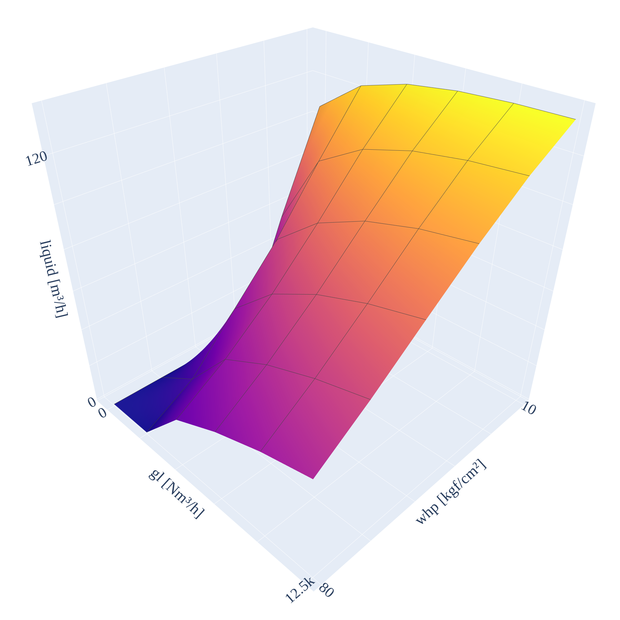
An example of the liquid flow function of a real well can be seen in Figure 1 with fixed values for and . As both and can be controlled, but have a nonlinear relationship with the outcome, we apply piecewise linearization to as a function of both. More precisely, let and be sets of indices for lift-gas injection and wellhead pressure. Let also and be the respective breakpoint values for well , and
| (2) |
be the liquid flow rates for the well at the breakpoints. is obtained by using Marlim as in Eq. (1) with the adjusted parameters and .
The piecewise approximation is then given by
| (3a) | ||||
| (3b) | ||||
| (3c) | ||||
| (3d) | ||||
| (3e) | ||||
To ensure piecewise linearization, SOS2 constraints are necessary for the values of that correspond to and , as follows
| (4a) | ||||
| (4b) | ||||
| (4c) | ||||
| (4d) | ||||
SOS2 constraints imply that no more than two consecutive elements of the ordered set of variables are nonzero (Beale and Tomlin, 1969).
2.3 Problem formulation
All oil wells are connected to a hub that directs their liquid productions to separators. The separators then split the liquid flow into the oil, gas, and water phase flows. This separation depends on the BSW and GOR of each well ,
| (5a) | ||||
| (5b) | ||||
| (5c) | ||||
The total gas flow is limited by the maximum lift-gas flow available though
| (6) |
Finally, the objective is to maximize the total volume of oil extracted
| (7) |
We can express the problem as
| (8) |
where are the flow of lift-gas injected and the well-head pressure of each well.
Note that the problem, in this case using piecewise linearization of the liquid flow, is an MILP parameterized by , , , and . Therefore, let be the vector of problem parameters. We can write the problem as
| (9) |
where is the vector of continuous variables (e.g., , , ) and is the vector of binary variables necessary for the SOS2 constraints. More precisely, is such that, for all ,
| (10a) | ||||
| (10b) | ||||
| (10c) | ||||
| (10d) | ||||
| (10e) | ||||
| (10f) | ||||
| (10g) | ||||
| (10h) | ||||
| (10i) | ||||
in which if the -th interval is selected, meaning that and only and can be nonzero, otherwise assumes value . The semantics of the binary variables are analogous. Notice that, because is binary, the operator in (10d) can be equivalently represented by the linear form . The formulation (10) is equivalent to the SOS2 constraints in (4c) and (4d).
3 Methodology
3.1 Early fixing
Suppose we can determine which linearization region of is to be selected (i.e., which variables and can have nonzero values). In that case, the SOS2 constraints can be removed; thus, the problem becomes completely linear. This is equivalent to fixing the variables in the standard formulation (9). Therefore, let us write as the problem (9) but with fixed values, i.e., with integer variables treated as parameters.
An early fixing heuristic provides an assignment to the integer variables. Ideally, the assignment will be such that . Since the early-fixed problem is an LP, it can be solved much faster than the original MILP problem. Therefore, the total cost of solving the early-fixed problem is the cost of solving the LP and the cost of running the heuristic. In practice, however, a trade-off between the cost of running the heuristic and the gap between and is expected.
Our proposed approach is to develop an early fixing heuristic based on a deep-learning model. We want a deep learning model with which we can compute . Two distinct approaches to training such a model are proposed.
3.2 Supervised learning approach
We can train a model for early fixing by feeding it with instances of the MILP problem and optimizing the model’s parameters such that its output approximates the optimal binary assignment. Let us define a dataset
which associates instances’ parameter vectors with the optimal binary assignment . Note that this dataset requires us to solve to optimality all MILP instances available.
Let us define a deep learning model
| (11) |
for which is the vector of model parameters that can be trained. Then, it is possible to optimize the model’s parameters such that for each vector of parameters in , the model’s output approximates . Namely,
| (12) |
where can be, for example, the binary cross entropy between the elements of both vectors.
3.3 Weakly-supervised learning approach
We propose an alternative learning approach that does not require solving MILP problems. First, we recall that the target of the deep learning model is to provide such that is maximized111Since (9) is a maximization problem.. Our proposed approach is to train a surrogate model that approximates , and differentiate through this surrogate to train the early fixing heuristic using gradient descent methods.
This approach requires only a dataset of assignments for the integer variables paired with the objective of the respective early-fixed problem. Let us define
which is built with (random) samples of . Then, we train a model
| (13) |
in a supervised manner, such that its output approximates , that is,
| (14) |
where can be, for example, the mean squared error.
Now, let us define
| (15) |
which can be trained in an unsupervised manner to maximize the surrogate model’s output given the candidate values for fixing
| (16) |
where denotes that is chosen randomly from , and the summation is iterated over as many random samples as desired. Note that only is optimized during the training of , i.e., is unchanged.
4 Experiments and Results222Code available in github/brunompacheco/early-fixing-oil-production.
4.1 Data
For our experiments, we consider the problem of optimizing oil production from a single well (). We use data from a real subsea oil well, provided by Petrobras444The data is not made available as it is an intellectual property of Petrobras. . We set a target for the early fixing models to generalize to different values of , , and . Therefore, we describe the parameter space of our problem as
assuming that the BSW can be no lower than 0.5, the GOR is always smaller than 300, and the maximum lift-gas flow is always larger than . More precisely, we assume that, in practice, , , and . Note that we omit the liquid flow function from the parameter vector, once we deal with a single well and, thus, can be uniquely determined by the other parameters.
The liquid flow function is always linearized with the same breakpoints for both and . This makes the domain of the binary variables consistent across instances. The selected breakpoints are
| (17a) | |||||
| (17b) | |||||
An example of with these breakpoints can be seen in Figure 1. With the fixed breakpoints, we can describe the domain of the binary variables as
| (18) |
in which indicates the pair of variables that can take nonzero values, while indicates the pair of variables that can take nonzero values.
For the supervised learning task, we build with 500 instances of the MILP problem from different combinations of , , and . Gurobi was used to solve the MILPs, upon which , the optimal value for the binary variables, was extracted. We use the same vectors as in for the weakly-supervised learning task. For each we draw 12 random candidates , that is, we ensure that each respects the constraints in (10). Then, is built by solving the LPs using Gurobi to compute . Whenever and resulted in an infeasible problem, we added them to with . In total, contains 500 data points of the form , while contains 6000 data points of the form .
4.2 Supervised learning experiments
For supervised learning, using , we choose
| (19) |
where is the -dimensional simplex set, as a neural network with 2 hidden layers of neurons each and a -dimensional output. The inputs are normalized before the first layer. We use ReLU activation for all layers except the last one. The last layer’s output is divided into two vectors of dimension , passing through the softmax function, thus mapping both into 5-dimensional simplexes. The softmax in the output of the network ensures that, after rounding, it respects the binary constraints, that is, and respect (10).
We randomly split into training and test sets with an 80-20 ratio. The training data was used to select the optimal network architecture and hyperparameters (learning rate, batch size, and number of epochs). After this adjustment, the entirety of the training set was used to train models with random initialization. Adam is used to optimizing the parameters of the models on the training set such that is minimized (see equation (12)). We use
where BCE is the binary cross-entropy function. We use batches of elements and an initial learning rate of 0.001. Each model is trained for epochs. The performance on the test set is summarized in Table 1.
| Model | Accuracy | Infeasible | Objective gap |
|---|---|---|---|
| Supervised | 99.78% | 0.11% | 0.01% |
| Weakly-supervised | 32.31% | 4.19% | 3.64% |
| Baseline | 0% | 0% | 21.42% |
4.3 Weakly-supervised learning experiments
We build the surrogate model
| (20) |
as a neural network with hidden layers of neurons each. ReLU is used as an activation function at each layer except the last one, which has no activation function. Inputs are normalized and a factor of scales the output. Dropout is applied during training at each hidden layer with a probability of % for each neuron.
The dataset is split randomly into a training and test set following an 80-20 ratio. The optimal architecture and hyperparameters (learning rate, batch size, number of epochs) were determined in the same way as in Sec. 4.2. We use the squared error as the loss function
We use Adam to minimize the loss function on the training set, with an initial learning rate of and mini-batches of samples. models with random initialization are trained for epochs each. On the test set, the surrogate models correctly predicted the feasibility (its output was lower than ) an average of % of the time. The average MAE on the instances that were not infeasible was . Figure 2 shows an example of the surrogate model’s performance compared to the real objective values.

The early fixing model has the same architecture as . models with random initialization are trained as described in Section 3.3, but using the parameters from the training set of described above. Each model is trained with a different surrogate model . The models are trained using Adam with an initial learning rate of and a batch of for epochs each. The performance on the test set is reported in Table 1.
4.4 Baseline Model
As a reference for the deep learning models’ performance, we compute the results of always fixing the same values for the binary variables. In our problem, the safest option in this approach is always to pick the region with the smallest values possible for and . This always results in a feasible problem. The performance of this baseline approach on the test set of can be seen in Table 1.
4.5 Early Fixing Impacts
To evaluate the impacts of early fixing in the optimization, we measure the runtime of solving the original MILP, the runtime of the early-fixed problem (which is an LP), and the runtime of the early fixing models. We perform these experiments on all instances of , i.e., with the problems defined by the parameters in the dataset used in the experiments above.
We found that the original problem can be solved, on average, in 0.90 ms, while the early-fixed problem is solved in an average of 0.18 ms. Considering the 0.08 ms the early-fixing models took, on average, during the experiments, the early-fixing approach takes, on average, 0.26 ms, representing a 71.11% runtime reduction.
5 Conclusions
Our experiments show that deep-learning-based early fixing models successfully speed up the optimization of the offshore gas-lifted oil production problem, with a 71.11% runtime reduction. Training in a supervised learning setting, although with a significantly higher cost for collecting the training data, is undoubtedly a superior approach concerning the weakly-supervised setting. Nevertheless, the experiments with the weakly-supervised approach indicate that it is possible to develop an early fixing heuristic when optimal solutions to the MILPs are unavailable or too hard to obtain. Still, the weakly-supervised approach needs further refinement to achieve competitive results.
Further research is still necessary on the suitability of the deep-learning-based early fixing for harder problems, e.g., multiple wells connected to manifolds, with more operational constraints and more integer variables. Moreover, the early fixing approaches presented in this paper theoretically apply to any MILP. However, the performance of the models and the practical viability of them is still an open theme for research.
References
- Anderson et al. (2022) Anderson, L., Turner, M., and Koch, T. (2022). Generative deep learning for decision making in gas networks. Mathematical Methods of Operations Research, 95(3), 503–532. 10.1007/s00186-022-00777-x.
- Beale and Tomlin (1969) Beale, E. and Tomlin, J. (1969). Special facilities in a general mathematical programming system for nonconvex problems using ordered sets of variables. Operational Research, 69, 447–454.
- Bengio et al. (2021) Bengio, Y., Lodi, A., and Prouvost, A. (2021). Machine learning for combinatorial optimization: A methodological tour d’horizon. European Journal of Operational Research, 290(2), 405–421. 10.1016/j.ejor.2020.07.063.
- Ding et al. (2019) Ding, J.Y., Zhang, C., Shen, L., Li, S., Wang, B., Xu, Y., and Song, L. (2019). Accelerating primal solution findings for mixed integer programs based on solution prediction. 10.48550/arXiv.1906.09575.
- Lee and Mitchell (2009) Lee, E.K. and Mitchell, J.E. (2009). Integer Programming: Branch and Bound Methods. In C.A. Floudas and P.M. Pardalos (eds.), Encyclopedia of Optimization, 1634–1643. Springer US, Boston, MA. 10.1007/978-0-387-74759-0_286.
- Li and Wu (2022) Li, L. and Wu, B. (2022). Learning to accelerate approximate methods for solving integer programming via early fixing. 10.48550/arXiv.2207.02087.
- Luguesi et al. (2023) Luguesi, C., Camponogara, E., Seman, L.O., González, J.T., and Leithardt, V.R.Q. (2023). Derivative-free optimization with proxy models for oil production platforms sharing a subsea gas network. IEEE Access, 11, 8950–8967. 10.1109/ACCESS.2023.3239421.
- Müller et al. (2022) Müller, E.R., Camponogara, E., Seman, L.O., Hülse, E.O., Vieira, B.F., Miyatake, L.K., and Teixeira, A.F. (2022). Short-term steady-state production optimization of offshore oil platforms: wells with dual completion (gas-lift and ESP) and flow assurance. TOP, 30(1), 152–180. 10.1007/s11750-021-00604-2.
- Pacheco et al. (2023) Pacheco, B.M., Seman, L.O., Rigo, C.A., Camponogara, E., Bezerra, E.A., and dos Santos Coelho, L. (2023). Graph neural networks for the offline nanosatellite task scheduling problem. ArXiv:2303.13773 [cs.LG].
- Seman et al. (2020) Seman, L.O., Miyatake, L.K., Camponogara, E., Giuliani, C.M., and Vieira, B.F. (2020). Derivative-free parameter tuning for a well multiphase flow simulator. Journal of Petroleum Science and Engineering, 192, 107288. 10.1016/j.petrol.2020.107288.
- Vigerske and Gleixner (2018) Vigerske, S. and Gleixner, A. (2018). SCIP: global optimization of mixed-integer nonlinear programs in a branch-and-cut framework. Optimization Methods and Software, 33(3), 563–593. 10.1080/10556788.2017.1335312.