Deep-Learned Event Variables for Collider Phenomenology
Abstract
The choice of optimal event variables is crucial for achieving the maximal sensitivity of experimental analyses. Over time, physicists have derived suitable kinematic variables for many typical event topologies in collider physics. Here we introduce a deep learning technique to design good event variables, which are sensitive over a wide range of values for the unknown model parameters. We demonstrate that the neural networks trained with our technique on some simple event topologies are able to reproduce standard event variables like invariant mass, transverse mass, and stransverse mass. The method is automatable, completely general, and can be used to derive sensitive, previously unknown, event variables for other, more complex event topologies.
Introduction. Data in collider physics is very high-dimensional, which brings a number of challenges for the analysis, encapsulated in “the curse of dimensionality” [1]. Mapping the raw data to reconstructed objects involves initial dimensionality reduction in several stages, including track reconstruction, calorimeter clustering, jet reconstruction, etc. Subsequently, the kinematics of the reconstructed objects is used to define suitable analysis variables, adapted to the specific channel and targeted event topology. Each such step is essentially a human-engineered feature-extraction process from complicated data to a handful of physically meaningful quantities. While some information loss is unavoidable, physics principles and symmetries help keep it to a minimum.
In this letter, we shall focus on the last stage of this dimensionality reduction chain, namely, the optimal construction of kinematic variables, which is essential to expedite the discovery of new physics and/or to improve the precision of parameter measurements. By now, the experimentalist’s toolbox contains a large number of kinematic variables, which have been thoroughly tested in analyses with real data (see [2, 3, 4, 5] for reviews). The latest important addition to this set are the so-called “singularity variables” [6, 7, 8, 9, 10], which are applicable to missing energy events — the harbingers of dark matter production at colliders. In the machine learning era, a myriad of algorithms have been invented or adopted to tackle various tasks that arise in the analysis of collider data, e.g., signal–background discrimination (see [11] for a continuously updated complete review of the literature). Under the hood, the machines trained in these techniques could learn to construct useful features from the low-level event description, because they are relevant to the task at hand. But it is difficult to interpret what exactly the machines have learned in the process [12, 13]. Furthermore, it is rarely studied whether the human-engineered features are indeed the best event variables for certain purposes, and whether machines can outperform theorists at constructing event variables.
These two issues, explainability and optimality, are precisely the two questions which we shall address in this letter. We shall introduce a new technique for training neural networks to directly output useful features or event variables (which offer sensitivity over a range of unknown parameter values). This allows for explainability of the machine’s output by comparison against known features in the data. At the same time, it is important to verify that the variables obtained using our technique are indeed the optimal choice, and we will test this by directly comparing them against the human-engineered variables that are known to be optimal for their respective event topologies. Once we have validated our training procedure in this way, we could extend it to more complex event topologies and derive novel kinematic variables in interesting and difficult scenarios.
Understanding how and what a neural network (NN) learns is a difficult task. Here we shall consider relatively simple physics examples that are nevertheless highly non-trivial from a machine learning point of view: (1) visible two-body decay (to two visible daughter particles); (2) semi-invisible two-body decay (to one visible and one invisible daughter particle); (3) semi-invisible two-body decays of pair-produced particles. It is known that the relevant variables in those situations are the invariant mass , the transverse mass [14, 15] and the stransverse mass [16], respectively. We will demonstrate that in each case, the NN can be trained to learn the corresponding physics variable in the reduced latent space. The method can be readily generalized to more complex cases to derive deep-learned, next-generation event variables.
Methodology. Let represent the high-dimensional input features from a collision event, e.g., the 4-momenta of the reconstructed physics objects. Let be a low-dimensional event variable constructed from . In this work, we shall model the function using a neural network, where for notational convenience, the dependence of on the architecture and weights of the network will not be explicitly indicated. We imagine that retains the relevant physics information and will be the centerpiece of an experimental study of a theory model with a set of unknown parameters . The goal is to train the NN encoding the function to be “useful” over a wide range of values for . For this purpose, we will need to train with events generated from a range of values. Note that this is a departure from the traditional approach in particle physics, where training is done for specific study points with fixed values of . In addition, we will have to quantify the usefulness of a given event variable , as explained in the remainder of this section.
Intuition from Information Theory. Each event carries some information about the underlying model parameter values from which it was produced. Some of this information could be lost when reducing the dimensionality of the data from to , as a consequence of the data processing inequality [17]. Good event variables minimize this information loss, and efficiently retain the information about the underlying parameter values [18, 19]. This is precisely why the invariant mass , the transverse mass and the stransverse mass have been widely used in particle physics for mass parameter measurements and for new physics searches.
The mutual information of and is given by
| (1) |
where and are the probability distribution functions of and , respectively, and is their joint distribution. and are the domains of and , respectively. One can think of as the prior distribution of .111For convenience, we will adopt the Bayesian interpretation of probability in the presentation of this work. The distributions and can then be derived from and the conditional distribution .
The mutual information quantifies the amount of information contained in about . Therefore, a good event variable should have relatively high values of . From Eq. (1), one can see that is nothing but the Kullback–Leibler (KL) divergence from (a) the factorized distribution to (b) the joint distribution . The KL divergence, in turn, is a measure of how distinguishable the two distributions (a) and (b) are.
These observations lead to the following strategy schematically outlined in FIG. 1: train the event variable network so that the distributions and are highly distinguishable. An auxiliary classifier network can then be used for evaluating the distinguishability of the two distributions. The basic blueprint of our training technique will be described next.
Training Data Generation. In order to generate the training data, we start with the two distributions and . The specific choice of a prior distribution is not crucial — as long as it allows to sample over a sufficiently wide range (the one in which we want the event variable to be sensitive) any function will do, and one is further free to impose theoretical prejudice like fine tuning, etc.
is the distribution of the event conditional on . General purpose event generators can be used to sample from this distribution. The overall distribution of , namely , is given by
| (2) |
Our training data consists of two classes, whose generation is illustrated in the left (green) block of FIG. 1. Each training data point is given by a 2-tuple along with the class label of the data point. Under class 0, and are independent of each other and their joint distribution is given by . This is accomplished by simply replacing the true value of used to generate with a fake one for the datapoints in class 0. Under class 1, the joint distribution of is given by
| (3) |

Event Variable Training. As shown in the right (blue) block FIG. 1, we then set up a composite network for classifying the data points into the two classes. The composite network consists of two parts. First, an event variable network (EVN) takes the high-dimensional collider event information as input and returns a low-dimensional as output. As indicated, this network parameterizes the artificial event variable function , which is precisely what we are interested in training. The output layer of the EVN network does not use an activation function (or, equivalently, uses the identity activation). Since , the main task of the EVN network is to perform the needed dimensionality reduction. However, to ensure that this retains the maximal amount of information, we introduce an auxiliary classifier network which takes the event variable and the parameters as input and returns a one-dimensional output, . Note that the input received by the auxiliary network is distributed as under class 0, and as under class 1.
The information bottleneck [18] created by the EVN module is optimized by simply training the composite network as a classifier for the input data , using the class labels as the supervisory signal.
Experiments. The EVN module in the network architecture from FIG. 1 reduces the original -dimensional features to a -dimensional subspace of event variables, which by construction are guaranteed to be highly sensitive to the theory model parameters , but without any explicit dependence on them. Such variables have been greatly valued in collider phenomenology, and a significant number have been proposed and used in experimental analyses. As a proof of principle, we shall now demonstrate how our approach is able to reproduce the known kinematic variables in a few simple but non-trivial examples. Here we shall only consider one variable at a time, i.e., , postponing the case of to future work [20].
Example 1: Fully visible two-body decay. First we consider the fully visible decay of a parent particle into two massless visible daughter particles, . The parameter in this example is the mass of the mother particle . The event is specified by the 4-momenta of the daughter particles and , leading to .
The prior is chosen to sample uniformly in the range GeV. For each sampled value of , we generate an event as follows. A generic boost for the parent particle is obtained by isotropically picking the direction for its momentum and uniformly sampling its lab frame energy in the range . Subsequently, is decayed on-shell into two massless particles (isotropically in its own rest frame), so that the input data consists of the lab-frame final state 4-momenta .
All the neural networks used in this work were implemented in TensorFlow [21]. For the event variable network, we used a sequential fully connected architecture with 5 hidden layers. The hidden layers, in order, have 128, 64, 64, 64, and 32 nodes, all of them using ReLU as the activation function. The output layer has one node with no activation function. The classifier network is a fully connected network with 3 hidden layers (16 nodes each, ReLU activation). The output layer has one node with sigmoid activation. These two networks were combined as shown in the right (blue) block of FIG. 1 and trained with 2.5 million events total (50–50 split between classes 0 and 1), out of which 20% was set aside for validation. The network was trained for 20 epochs with a mini-batch size of 50, using the Adam optimizer and the binary crossentropy loss function.
For the event topology considered in this example, it is known that the event variable most sensitive to the value of is the invariant mass of the daughter particles
| (4) |
as well as any variable that is in one-to-one correspondence with it. In order to test whether our artificial event variable learned by the NN correlates with , we show a heatmap of the joint distribution of in the upper-left panel of FIG. 2. Here, and in what follows, the heatmap is generated using a separate test dataset with events. In the plot we also show two nonparametric correlation coefficients, namely Kendall’s coefficient [22] and Spearman’s rank correlation coefficients [23]. A value of for them would indicate one-to-one correspondence. Our results depict an almost perfect correspondence between and . Here, and in what follows, we append an overall minus sign to if needed, to make the correlations positive and the plots in FIG. 2 intuitive.


In practice, the artificial variable can be used to compare the data against templates simulated for different values of . To illustrate this usage, in the lower-left panel of FIG. 2 we show unit-normalized distributions of the deep-learned variable for several different values of GeV. It is seen that the distributions are highly sensitive to the parameter choice and, if needed, can be calibrated so that the peak location directly corresponds to . The observed spread around the peak values in the histogram, as well as the less than perfect correspondence between and , are due to limitations in the NN architecture and training.
Example 2: Semi-visible two body decay. Next we consider the semi-visible two-body decay of a particle into a massless visible particle and a possibly massive invisible particle , , where is singly produced (with zero transverse momentum). The parameter is two-dimensional: . The event is specified by the 4-momentum of and the missing transverse momentum, leading to .
We generate by uniformly sampling in the region defined by and , where . This choice of prior ensures that the relevant mass difference parameter in this event topology is adequately sampled in the range GeV. For the given value of , we generate an event as follows. The parent particle is boosted along the beam axis (with equal probability) to an energy chosen uniformly in the range . The particle is decayed on-shell into and , isotropically in its own rest frame. The details of network architectures and training are the same as in Example 1.
The relevant variable for this event topology is the transverse mass , which in our setup is given by
| (5) |
where the choice of mass ansatz for the mass of the invisible particle does not affect the rank ordering of the events. For concreteness in what follows we shall use . The corresponding heatmap of the joint distribution and unit-normalized distributions of the variable for several choices of GeV and GeV are shown in the middle panels of FIG. 2. Once again, we observe an almost perfect correlation between and , and a high sensitivity of the distributions to the input masses.
Example 3: Symmetric semi-visible two body decays. Finally, we consider the exclusive production at a hadron collider of two equal-mass parent particles and which decay semi-visibly as . The parameter is given by , and the event is described by the 4-momemta of and , and the missing transverse momentum, leading to .
The masses are generated as in Example 2. In order to avoid fine turning the network to the details of a particular collider, we uniformly sampled the invariant mass of the system in the range and the lab-frame energy of the system in the range . The direction of the system was chosen to be along with equal probability. The direction of is chosen isotropically in the rest frame of the system. and are both decayed on-shell, isotropically in their respective rest frames. The details of network architectures and training are the same as in Example 1.
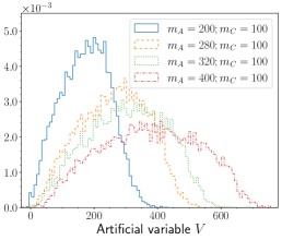
The straightforward generalization of the idea of the transverse mass to the considered event topology leads to the stransverse mass variable [16]. In the upper-right panel of FIG. 2 we show a heatmap of the joint distribution of , which reveals reasonably good, but not perfect correlation, implying that the artificial event variable encapsulates information beyond . This could have been expected for the following two reasons: 1) unlike the previous two examples of singular variables with sharp features in their distributions, does not belong to the class of singular variables [10]; 2) only uses a subset of the available kinematic information, namely the transverse momentum components. In contrast, the artificial kinematic variable can use all of the available information, and in a more optimal way. The lower-right panel of FIG. 2 displays unit-normalized distributions of the artificial variable for several choices of and fixed GeV, again demonstrating the sensitivity of to the mass spectrum.
Discussion and outlook. We proposed a new deep learning technique pictorially summarized in FIG. 1 which allows the construction of event variables from a set of training data produced from a given event topology. The novel component is the simultaneous training for varying parameters which allows the algorithm to capture the underlying phase space structure irrespective of the benchmark study point. This is the first such method for constructing event variables with neural networks and can be applied to other, more challenging event topologies in particle physics and beyond. In future applications of the method one could enlarge the dimensionality of the latent space to and supplement the training data with additional features like tagging and timing information, etc. By manipulating the specifics of the generation of the training data, one can control what underlying physics effects are available for the machine to learn from, and what physical parameters the machine-learned variable will be sensitive to. Our method opens the door to new investigations on intepretability and explainability by incorporating modern representation learning approaches like contrastive learning [24].
Code and Data Availability. The code and data that support the findings of this study are openly available at the following URL: https://gitlab.com/prasanthcakewalk/code-and-data-availability/ under the directory named arXiv_2105.xxxxx.
Acknowledgements
We are indebted to the late Luc Pape for great insights and inspiration. This work is supported in parts by US DOE DE-SC0021447 and DE-FG02-13ER41976. MP is supported by Basic Science Research Program through the National Research Foundation of Korea Research Grant No. NRF-2021R1A2C4002551. PS is partially supported by the U.S. Department of Energy, Office of Science, Office of High Energy Physics QuantISED program under the grants “HEP Machine Learning and Optimization Go Quantum”, Award Number 0000240323, and “DOE QuantiSED Consortium QCCFP-QMLQCF”, Award Number DE-SC0019219.
This manuscript has been authored by Fermi Research Alliance, LLC under Contract No. DEAC02-07CH11359 with the U.S. Department of Energy, Office of Science, Office of High Energy Physics.
References
- [1] R. Bellman, “Dynamic Programming”, Princeton University Press, 1957.
- [2] T. Han, “Collider phenomenology: Basic knowledge and techniques,” [arXiv:hep-ph/0508097 [hep-ph]].
- [3] A. J. Barr and C. G. Lester, “A Review of the Mass Measurement Techniques proposed for the Large Hadron Collider,” J. Phys. G 37, 123001 (2010) [arXiv:1004.2732 [hep-ph]].
- [4] A. J. Barr, T. J. Khoo, P. Konar, K. Kong, C. G. Lester, K. T. Matchev and M. Park, “Guide to transverse projections and mass-constraining variables,” Phys. Rev. D 84, 095031 (2011) [arXiv:1105.2977 [hep-ph]].
- [5] K. T. Matchev, F. Moortgat and L. Pape, “Dreaming Awake: Disentangling the Underlying Physics in Case of a SUSY-like Discovery at the LHC,” J. Phys. G 46, no.11, 115002 (2019) [arXiv:1902.11267 [hep-ph]].
- [6] I. W. Kim, “Algebraic Singularity Method for Mass Measurement with Missing Energy,” Phys. Rev. Lett. 104, 081601 (2010) [arXiv:0910.1149 [hep-ph]].
- [7] A. Rujula and A. Galindo, “Measuring the W-Boson mass at a hadron collider: a study of phase-space singularity methods,” JHEP 08, 023 (2011) [arXiv:1106.0396 [hep-ph]].
- [8] A. De Rujula and A. Galindo, “Singular ways to search for the Higgs boson,” JHEP 06, 091 (2012) [arXiv:1202.2552 [hep-ph]].
- [9] D. Kim, K. T. Matchev and P. Shyamsundar, “Kinematic Focus Point Method for Particle Mass Measurements in Missing Energy Events,” JHEP 10, 154 (2019) [arXiv:1906.02821 [hep-ph]].
- [10] K. T. Matchev and P. Shyamsundar, “Singularity Variables for Missing Energy Event Kinematics,” JHEP 04, 027 (2020) [arXiv:1911.01913 [hep-ph]].
- [11] M. Feickert and B. Nachman, “A Living Review of Machine Learning for Particle Physics,” [arXiv:2102.02770 [hep-ph]].
- [12] S. Chang, T. Cohen and B. Ostdiek, “What is the Machine Learning?,” Phys. Rev. D 97, no.5, 056009 (2018) [arXiv:1709.10106 [hep-ph]].
- [13] T. Faucett, J. Thaler and D. Whiteson, “Mapping Machine-Learned Physics into a Human-Readable Space,” Phys. Rev. D 103, no.3, 036020 (2021) [arXiv:2010.11998 [hep-ph]].
- [14] V. D. Barger, A. D. Martin and R. J. N. Phillips, “Perpendicular Mass From Decay,” Z. Phys. C 21, 99 (1983).
- [15] J. Smith, W. L. van Neerven and J. A. M. Vermaseren, “The Transverse Mass and Width of the Boson,” Phys. Rev. Lett. 50, 1738 (1983).
- [16] C. G. Lester and D. J. Summers, “Measuring masses of semiinvisibly decaying particles pair produced at hadron colliders,” Phys. Lett. B 463, 99-103 (1999) [arXiv:hep-ph/9906349 [hep-ph]].
- [17] N. Beaudry, “An intuitive proof of the data processing inequality,” Quantum Information & Computation, 12 (5–6): 432–441 (2012) [arXiv:1107.0740 [quant-ph]].
- [18] N. Tishby, F. C. Pereira and W. Bialek, “The information bottleneck method”, Proc. of the 37-th Annual Allerton Conference on Communication, Control and Computing, page 368-377, (1999), [arXiv:physics/0004057 [physics.data-an]].
- [19] R. Iten, T. Metger, H. Wilming, L. del Rio, R. Renner, “Discovering physical concepts with neural networks,” Phys. Rev. Lett. 124, 010508 (2020), [arXiv:1807.10300 [quant-ph]].
- [20] D. Kim, K. Kong, K. T. Matchev, M. Park and P. Shyamsundar, in preparation.
- [21] Martín Abadi, et. al,“Large-Scale Machine Learning on Heterogeneous Systems,” https://www.tensorflow.org/.
- [22] Maurice G. Kendall, “The treatment of ties in ranking problems”, Biometrika Vol. 33, No. 3, pp. 239-251. 1945.
- [23] Zwillinger, D. and Kokoska, S. “CRC Standard Probability and Statistics Tables and Formulae”. Chapman & Hall: New York. 2000. Section 14.7.
- [24] P. Le-Khac, G. Healy and A. Smeaton, “Contrastive Representation Learning: A Framework and Review,” IEEE Access, vol. 8, pp. 193907-193934, 2020, [arXiv:2010.05113 [cs.LG]].