Deep Latent-Variable Kernel Learning
Abstract
Deep kernel learning (DKL) leverages the connection between Gaussian process (GP) and neural networks (NN) to build an end-to-end, hybrid model. It combines the capability of NN to learn rich representations under massive data and the non-parametric property of GP to achieve automatic regularization that incorporates a trade-off between model fit and model complexity. However, the deterministic encoder may weaken the model regularization of the following GP part, especially on small datasets, due to the free latent representation. We therefore present a complete deep latent-variable kernel learning (DLVKL) model wherein the latent variables perform stochastic encoding for regularized representation. We further enhance the DLVKL from two aspects: (i) the expressive variational posterior through neural stochastic differential equation (NSDE) to improve the approximation quality, and (ii) the hybrid prior taking knowledge from both the SDE prior and the posterior to arrive at a flexible trade-off. Intensive experiments imply that the DLVKL-NSDE performs similarly to the well calibrated GP on small datasets, and outperforms existing deep GPs on large datasets.
Index Terms:
Gaussian process, Neural network, Latent variable, Regularization, Hybrid prior, Neural stochastic differential equation.I Introduction
In the machine learning community, Gaussian process (GP) [1] is a well-known Bayesian model to learn the underlying function . In comparison to the deterministic, parametric machine learning models, e.g., neural networks (NN), the non-parametric GP could encode user’s prior knowledge, calibrate the model complexity automatically, and quantify the uncertainty of prediction, thus showing high flexibility and interpretability. Hence, it has been popularized within various scenarios like regression, classification [2], clustering [3], representation learning [4], sequence learning [5], multi-task learning [6], active learning and optimization [7, 8].
However, the two main weaknesses of GP are its poor scalability and the limited model capability on massive data. Firstly, as an representative of kernel method, the GP employs the kernel function to encode the spatial correlations of training points into the stochastic process. Consequently, it performs operations on the full-rank kernel matrix , thus raising a cubic time complexity which prohibits the application in the era of big data. To improve the scalability, various scalable GPs have then been presented and studied. For example, the sparse approximations introduce () inducing variables to distillate the latent function values through prior or posterior approximation [9, 10], thus reducing the time complexity to . The variational inference with reorganized evidence lower bound (ELBO) could further make the stochastic gradient descent optimizer, e.g., Adam [11], available for training with a greatly reduce complexity of [12]. Moreover, further complexity reduction can be achieved by exploiting the structured inducing points and the iterative methods through matrix-vector multiplies, see for example [13, 14]. In contrast to the global sparse approximation, the complexity of GP can also be reduced through distributed computation [15, 16] and local approximation [17, 18]. The idea of divide-and-conquer splits the data for subspace learning, which alleviates the computational burden and helps capturing local patterns. The readers can refer to a recent review [19] of scalable GPs for further information.
Secondly, the GP usually uses (i) the Gaussian assumption to have closed-form inference, and (ii) the stationary and smoothing kernels to simply quantify how quickly the correlations vary along dimensions, which thus raise urgent demand for developing new GP paradigms to learn rich statistical representations under massive data. Hence, the interpretation of NN from kernel learning [20] inspires the construction of deep kernels for GP to mimic the nonlinearity and recurrency behaviors of NN [21, 22]. But the representation learning of deep kernels in comparison to deep models reviewed below is limited unless they are richly parameterized [23].
Considering the theoretical connection between GP and wide deep neural networks [24, 25], a hybrid, end-to-end model, called deep kernel learning (DKL) [26, 27, 28], has been proposed to combine the non-parametric property of GP and the inductive biases of NN. In this framework, the NN plays as a deterministic encoder for representation learning, and the sparse GP is built on the latent inputs for providing Bayesian estimations. The NN+GP structure thereafter has been extended for handling semi-supervised learning [29] and time-series forecasting [30]. The automatic regularization through the marginal likelihood of the last GP layer is expected to improve the performance of DKL and reduces the requirement of fine-tuning and regularization. But we find that the deterministic encoder may deteriorate the regularization of DKL, especially on small datasets, which will be elaborated in the following sections. Alternatively, we could stack the sparse GPs together to build the deep GP (DGP) [31, 32], which admits the layer-by-layer GP transformation that yields non-Gaussian distributions. Hence, the DGPs usually resort to the variational inference for model training. Different from DKL, the DGPs employ the full GP paradigm to arrive at automatic regularization. But the representation learning through layer-by-layer sparse GPs suffers from (i) high time complexity, (ii) complicated approximate inference, and (iii) limited capability due to the finite global inducing variables in each layer.
From the foregoing review and discussion, it is observed that the simple and scalable DKL enjoys great representation power of NN but suffers from the mismatch between the deterministic representation and the stochastic inference, which may risk over-fitting, especially on small datasets. While the sparse DGP enjoys the well calibrated GP paradigm but suffers from high complexity and limited representation capability.
Therefore, this article presents a complete Bayesian version of DKL which inherits (i) the scalability and representation of DKL and (ii) the regularization of DGP. The main contributions of this article are three-fold:
-
•
We propose an end-to-end latent-variable framework called deep latent-variable kernel learning (DLVKL). It incorporates a stochastic encoding process for regularized representation learning and a sparse GP part for guarding against over-fitting. The whole stochastic framework ensures that it can fully benefit from the automatic regularization of GP;
-
•
We further improve the DLVKL by constructing (i) the informative variational posterior rather than the simple Gaussian through neural stochastic differential equations (NSDE) to reduce the gap to exact posterior, and (ii) the flexible prior incorporating the knowledge from both the SDE prior and the variational posterior to arrive at a trade-off. The NSDE transformation improves the representation learning and the trade-off provides an adjustable regularization in various scenarios;
-
•
We showcase the superiority of DLVKL-NSDE against existing deep GPs through intensive (un)supervised learning tasks. The tensorflow implementations are available at https://github.com/LiuHaiTao01/DLVKL.
The remainder of the article is organized as follows. Section II briefly introduces the sparse GPs. Section III then presents the framework of DLVKL. Thereafter, Section IV proposes an enhanced version, named DLVKL-NSDE, through informative posterior and flexible prior. Then extensive numerical experiments are conducted in Section V to verify the superiority of DLVKL-NSDE on (un)supervised learning tasks. Finally, Section VI offers the concluding remarks.
II Scalable GPs revisited
Let be the collection of points in the input space , and the observations in the output space , we seek to infer the latent mappings from data . To this end, the GP characterizes the distributions of latent functions by placing independent zero-mean GP priors as , . For regression and binary classification, we usually have ; while for multi-class classification and unsupervised learning, we are often facing .
We are interested in two statistics in the GP paradigm. The first is the marginal likelihood , where with .111For the sake of simplicity, we here use the same kernel for outputs. The marginal likelihood , the maximization of which optimizes the hyperparameters, automatically achieves a trade-off between model fit and model complexity [1]. As for , we adopt the Gaussian likelihood for regression and unsupervised learning with continuous outputs given the i.i.d noise [1, 4]. While for binary classification with discrete outputs and multi-class classification with , we have and , respectively, wherein is an inverse link function that squashes into the class probability space [33].
The second interested statistic is the posterior used to perform prediction at a test point as . Note that for non-Gaussian likelihoods, the posterior is intractable and we resort to approximate inference algorithms [34].
The scalability of GPs however is severely limited on massive data, since the inversion and determinant of incur operations. Hence, the sparse approximation [19] employs a set of inducing variables with at to distillate the latent function values . Then, we have
where and . Thereafter, variational inference could help handle the intractable . This is conducted by using a tractable variational posterior , and maximizing the KL divergence
where and . It is equivalent to maximizing the following ELBO
| (1) |
The likelihood term of represents the fitting error, and it factorizes over both data points and dimensions
thus having a remarkably reduced time complexity of when performing stochastic optimization. Note that is conditioned on the whole training points, where and . While the posterior only depends on the related point , where collects the -th element from each in the set ; and collects the -th diagonal element from each in the set .222This viewpoint inspires the doubly stochastic variational inference [32]. Besides, the covariance here is summarized by the inducing variables. Besides, the analytical KL term in (1) guards against over-fitting and seeks to deliver a good inducing set. Note that the likelihood in (1) is not limited to Gaussian. By carefully reorganizing the formulations, we could derive analytical expressions for for (un)supervised learning tasks [12, 35, 36].
III Deep latent-variable kernel learning
We consider a GP with additional -dimensional latent variables as333We could describe most of deep GPs by the model (3), see Appendix A.
| (3) |
where the conditional distribution indicates a stochastic encoding of the original input , which could ease the inference of the following generative model . As a result, the log marginal likelihood satisfies
| (4) |
In (4),
-
•
as for , we use independent GPs , , to fit the mappings between and . Consequently, we have the following lower bound by resorting to the sparse GP as
(5) Note that the GP mapping employed here learns a joint distribution by considering the correlations over the entire space in order to achieve automatic regularization;
-
•
as for the prior , we usually employ the fully independent form factorized over both data index and dimension index ;
-
•
as for the decoder , since we aim to utilize the great representational power of NN, it often takes the independent Gaussians . Instead of directly treating the means and variances as hyperparameters, they are made of parameterized function of the input through multi-layer perception (MLP), for example, as
This strategy is called amortized variational inference that shares the parameters over all training points, thus allowing for efficient training.
Combing (4) and (5), the final ELBO for the proposed deep latent-variable kernel learning (DLVKL) writes as
| (6) | ||||
which can be optimized by the reparameterization trick [38].
It is found that in comparison to the ELBO of DKL in Appendix A-A, the additional in (6) regularizes the representation learning of encoder, which distinguishes our DLVKL from the DKL proposed in [26]. The DKL adopts a deterministic representation learning , which is equivalent to the variational distribution . Intuitively, in order to maximize , it is encouraged to learn a which maps to a distribution concentrated on . Particularly, pushing all the mass of the distribution on results in , which however risks severe over-fitting [39]. The last GP layer employed in DKL is expected to alleviate this issue by considering the joint correlations over the output space. But the deterministic encoder, which is inconsistent to the following stochastic GP part, will incur free latent representation to weaken the model regularization, which results in over-fitting and under-estimated prediction variance in scenarios with finite data points. Contrarily, the proposed DLVKL builds a complete statistical learning framework wherein the additional KL regularization could avoid the issue by pushing to match the prior .
Note that when is unobservable, i.e., , the proposed DLVKL recovers the GPLVM using back constraints (recognition model) [40]. Also, the bound (6) becomes the VAE-type ELBO
| (7) | ||||
for unsupervised learning [38], wherein the main difference is that a GP decoder is employed.
Though the complete stochastic framework makes DLVKL be more attractive than DKL, it has two challenges to be addressed:
-
•
firstly, the assumed variational Gaussian posterior is often significantly different from the exact posterior . This gap may deteriorate the performance and thus raises the demand of expressive for better approximation, which will be addressed in Section IV-A;
-
•
secondly, the choice of prior affects the regularization on latent representation. The flexibility and expressivity of the prior will be improved in Section IV-B.
IV Improvements of DLVKL
The improvements of DLVKL come from two aspects: (i) the more expressive variational posterior transformed through neural stochastic differential equation (NSDE) for better approximating the exact posterior; and (ii) the flexible, hybrid prior to introduce adjustable regularization on latent representation. The two improvements are elaborated respectively in the following subsections.
IV-A Expressive variational posterior via NSDE
In order to generate expressive posterior rather than the simple Gaussian, which is beneficial for minimizing , we interpret the stochastic encoding as a continuous-time dynamic system governed by SDE [41] over the time period as
| (8) |
where the initial state ; is the deterministic drift vector; with is the positive definite diffusion matrix which indicates the scale of the random Brownian motion that scatters the state with random perturbation; and represents the standard and uncorrelated Brownian process, which starts from a zero initial state and has independent Gaussian increment .
The SDE flow in (8) defines a sequence of transformation indexed on a continuous-time domain, the purpose of which is to evolve the simple initial state to the one with expressive distribution. In comparison to the normalizing flow [42] indexed on a discrete-time domain, the SDE flow is more theoretically grounded since it could approach any distribution asymptotically [43]. Besides, the diffusion term, which distinguishes SDE from the ordinary differential equation (ODE) [44], makes the flow more stable and robust from the view of regularization [45].
The solution of SDE is given by the Itô integral which integrates the state from the initial state to time as
Note that due to the non-differentiable , the SDE yields continuous but non-smooth trajectories . Practically, we usually work with the Euler-Maruyama scheme for time discretization in order to solve the SDE system. Suppose we have time points in the period , they are equally spaced with time window . Then we have a generative transition between two conservative states
This is equivalent to the following Gaussian transition, given , as
| (9) |
Note that though the transition is Gaussian, the SDE finally outputs expressive posterior rather than the simple Gaussian, at the cost of however having no closed-form expression for . But the related samples can be obtained by solving the SDE system via the Euler-Maruyama method.
As for the drift and diffusion, alternatively, they could be represented by the mean and variance of sparse GP to describe the SDE field [46], resulting in analytical KL terms in ELBO, see Appendix A-C. In order to enhance the representation learning, we herein build a more powerful SDE with NN-formed drift and diffusion, called neural SDE (NSDE). This however comes at the cost of intractable KL term. It is found that the SDE transformation gives the following ELBO as
| (10) | ||||
Different from the ELBO in (6) which poses a Gaussian assumption for , the second KL term in the right-hand side of is now intractable due to the implicit density . Alternatively, it can be estimated through the obtained SDE trajectory samples as
| (11) |
To estimate the implicit density , Chen et al. [43] used the simple empirical method according to the SDE samples as , where is a point mass at . The estimation quality of this empirical method however is not guaranteed. It is found that since
| (12) |
we could evaluate the density through the SDE trajectory samples from the previous time as
| (13) | ||||
In practice, we adopt the single-sample approximation together with the reparameterization trick to perform backprogate and have an unbiased estimation of the gradients [38].
IV-B Flexible prior
IV-B1 How about an i.i.d prior?
Without apriori knowledge, we could simply choose an i.i.d prior with isotropic unit Gaussians. This kind of prior however is found to impede our model.
As stated before, when is unobservable, the bound (7) becomes the VAE-type ELBO for unsupervised learning. From the view of VAE, it is found that this ELBO may not guide the model to learn a good latent representation. The VAE is known to suffer from the issue of posterior collapse (also called KL vanishing) [47]. That is, the learned posterior is independent of the input , i.e., . As a result, the latent variable does not encode any information from . This issue is mainly attributed to the optimization challenge of VAE [48]. It is observed that maximizing the ELBO (7) requires minimizing , which favors the posterior collapse in the initial training stage since it gives a zero KL value. In this case, if we are using a highly expressive decoder which is capable of modeling arbitrarily data distribution, e.g., the PixelCNN [49], then the decoder will not use information from .
As for our model, though the GP decoder is not so highly expressive, it cannot escape from the posterior collapse due to the property of GP. Furthermore, the posterior collapse of our model has been observed even in supervised learning scenario, see Fig. 2. We will prove below that the DLVKL using the simple i.i.d prior suffers from a non-trivial state when posterior collapse happens.
Before proceeding, we make some required clarifications. First, it is known that the positions of inducing variables fall into the latent space . They are regarded as the variational parameters of and need to be optimized. However, since the latent space is not known in advance and it dynamically evolves through training, it is hard to properly initialize , which in turn may deteriorate the training quality. Hence, we employ the encoded inducing strategy indicated as below.
Definition 1.
(Encoded inducing) It puts the positions of inducing variables into the original input space instead of , and then passes them through the encoder to obtain the related inducing positions in the latent space as
Now the inducing positions take into account the characteristics of latent space through encoder and become Gaussians.
Second, the GP part employs the stationary kernel, e.g., the RBF kernel, for learning. The properties of stationary kernel are indicated as below.
Definition 2.
(Stationary kernel) The stationary kernel for GP is a function of the relative distance . Specifically, it is expressed as , where is the kernel parameters which mainly control the smoothness along dimensions, and is the output-scale amplitude. Particularly, the stationary kernel satisfies and .
Thereafter, the following proposition reveals that the DLVKL using i.i.d prior fails when posterior collapse happens.
Proposition 1.
Given the training data , we build a DLVKL model using the i.i.d prior , the stationary kernel and the encoded inducing strategy. When the posterior collapse happens in the initial stage of the training process, the DLVKL falls into a non-trivial state: it degenerates to a constant predictor, and the optimizer can only calibrate the prediction variance.
Detailed proof of this proposition is provided in Appendix C. Furthermore, it is found that for any i.i.d. prior , the degeneration in Proposition 1 happens due to the collapsed kernel matrices. The above analysis indicates that the simple i.i.d. prior impedes our model when posterior collapse happens. Though recently more informative priors have been proposed, for example, the mixture of Gaussians prior and the VampPrior [50], they still belong to the i.i.d. prior. This motivates us to come up with flexible and informative prior in order to avoid the posterior collapse.
IV-B2 A hybrid prior brings adjustable regularization
Interestingly, we could set the prior drift and diffusion , and let pass through the SDE system to have an analytical prior at time as
| (14) | ||||
The independent but not identically distributed SDE prior is more informative than . For this SDE prior,
-
•
it varies over data points, and will not incur the collapsed kernel matrices like the i.i.d prior, thus sidestepping the posterior collapse, see the empirical demonstration in Fig. 2; and
- •
Besides, the additional variance in the SDE prior is used to build connection to the posterior. For the posterior , we employ the following drift and diffusion for transition as
| (15) | ||||
The connection through allows knowledge transfer between the prior and the posterior, thus further improving the flexibility of the SDE prior.
More generally, it is found that for the independent but not identically distributed prior , the optimal choice for maximizing ELBO is . But this will cancel the KL regularizer and risk severe over-fitting. Alternatively, we could construct a composited prior, like [52], as
| (16) |
where is a trade-off parameter, and is a normalizer. When , we are using the SDE prior; when is a mild value, we are using a hybrid prior taking information from both the SDE prior and the variational posterior; when , we are using the variational posterior as prior.
The mixed prior gives the KL term regarding in as
| (17) | ||||
Note that the term has no trainable parameters. Thereafter, the ELBO rewrites to
| (18) | ||||
The formulation of -ELBO in (18) on the other hand indicates that can be interpreted as a trade-off between the likelihood (data fit) and the KL regularizer w.r.t , which is similar to [53]. This raises an adjustable regularization on the latent representation : when , the SDE prior poses the most strict regularization; when , the optimal prior ignores the KL regularizer, like DKL, and focuses on fitting the training data. It is recommended to use an intermediate , e.g., , to achieve a good trade-off; or an annealing- strategy [54, 55]. Note that the -ELBO can also be derived from the view of variational information bottleneck (VIB) [56], see Appendix B.
IV-C Discussions
Fig. 1 illustrates the structure of the proposed DLVKL and DLVKL-NSDE. It is found that the DLVKL is a special case of DLVKL-NSDE: when and , becomes Gaussian. Compared to the DLVKL, the DLVKL-NSDE generates more expressive variational posterior through NSDE, which is beneficial to further reduce the gap to the exact posterior. However, the NSDE transformation requires that the states should have the same dimensionality over time. It makes DLVKL-NSDE unsuitable for handling high-dimensional data, e.g., images. This however is not an issue for DLVKL since it has no limits on the dimensionality of . Besides, it is notable that when the encoder has , we cannot directly use the SDE prior (14). Alternatively, we could apply some simple dimensionality reduction algorithms, e.g., the principle component analysis (PCA), on the inputs to obtain the prior mean. When , we use the zero-padding strategy to obtain the prior mean. In the experiments below, unless otherwise indicated, we use the DLVKL-NSDE with , , and . When predicting, we average over posterior samples.

V Numerical experiments
This section first uses two toy cases to investigate the characteristics of the proposed models, followed by intensive evaluation on nine regression and classification datasets. Finally, we also simply showcase the capability of unsupervised DLVKL on the dataset. The model configurations in the experimental study are detailed in Appendix D. All the experiments are performed on a windows workstation with twelve 3.50 GHz core and 64 GB memory.
V-A Toy cases
This section seeks to investigate the characteristics of the proposed models on two toy cases. Firstly, we illustrate the benefits brought by the flexible prior and the expressive posterior on a regression case expressed as
which has a step behavior at the origin. The conventional GP using stationary kernels is hard to capture this non-stationary behavior. We draw 50 points from together with their observations as training data.
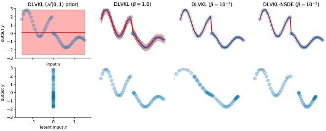
Fig. 2 illustrates the predictions of DLVKL and DLVKL-NSDE, together with the mean of the learned latent input . It is found, from left to right, that the i.i.d prior leads to collapsed posterior and constant predictor, which agree with the analysis in Proposition 1. Instead, the independent but not identically distributed SDE prior in (14) helps the DLVKL sidestep the posterior collapse. But since this prior takes no knowledge from the posterior under , the DLVKL leaves almost no space for the encoder to perform deep representation learning, which is crucial for capturing the step feature. As a result, the pure SDE prior makes DLVKL perform like a GP. Hence, to improve the capability of encoder, we employ the -mixed flexible prior in (16), which takes both the SDE prior and the variational posterior into consideration. Now we can observe that the encoder under skews the original inputs in the latent space in order to make the GP part of DLVKL describe the step behavior easily. Moreover, the DLVKL-NSDE further employs the NSDE-transformed variational posterior rather than the Gaussian, thus resulting in better latent representation.
Next, Fig. 3 investigates the impact of on the behavior of DLVKL-NSDE on a toy binary classification case by changing it from to . We also show the results of stochastic variational GP (SVGP) [12] and DKL for comparison. It is observed that the decreasing changes the behavior of DLVKL-NSDE from SVGP to DKL. The decreasing indicates that (a) the prior contains more information from the posterior, and it has when , like DKL; (b) the KL penalty w.r.t is weakened in (18), thus risking over-fitting; and meanwhile, (c) the encoder becomes more flexible, e.g., the extreme skews the 2D inputs to an almost 1D manifold, raising the issue of rank pathologies in deep models [23]. In practice, we need to trade off the KL regularization for guarding against over-fitting and the representation learning for improving model capability through the value.

Finally, Fig. 4 investigates the impact of SDE flow parameters and on the performance of DLVKL-NSDE. We first fix the flow time as and increase the flow step from to . When we directly use , (DLVKL-NSDE herein degenerates to DLVKL), it leads to a single transition density with large variance, thus resulting in high degree of feature skewness. This in turn raises slight over-fitting in Fig. 4 as it identifies several orange points within the blue group. In contrast, the refinement of flow step makes the time discretization close to the underlying process and stabilizes the SDE solver. Secondly, we fix the flow step as and increase the flow time from to . This increases the time window and makes the transition density having larger variance. Hence, the encoder is equipped with higher perturbation. But purely increasing will deteriorate the quality of SDE solver, which is indicated by the issue of rank pathologies for DLVKL-NSDE with , . To summarize, in order to gain benefits from the SDE representation learning, the flow step should increase with flow time . For example, in comparison to the case of and , the DLVKL-NSDE using and in Fig. 4 yields reasonable predictions and latent representation.

V-B Regression and classification
We here evaluate the proposed model on six UCI regression datasets, two classification datasets and the - image classification dataset summarized in Table I. The data size ranges from 506 to 11M in order to conduct intensive comparison at different levels. It is notable that the first three small regression datasets in Table I could help verify whether the proposed model can achieve reasonable regularization to guard against over-fitting or not.
The competitors include the pure SVGP [12] and NN, the DiffGP [46], a SDE-based deep GP, and finally the DKL [26]. For the regression tasks, we employ the root mean square error (RMSE) and the negative log likelihood (NLL) as performance criteria to quantify the quality of predictive distribution. Similarly, we verify the performance of classification in terms of classification accuracy and NLL. Tables II and III report the comparative results in terms of RMSE (accuracy) and NLL, respectively.444We only provide the RMSE and accuracy results for the deterministic NN. Besides, the SVGP and DiffGP are not applied on the - dataset, since the pure GPs cannot effectively handle the high-dimensional image data. The best and second-best results are marked in gray and light gray, respectively. Based on the comparative results, we have the following findings.
| dataset | no. of classes | |||
| boston | 456 | 50 | 13 | - |
| concrete | 927 | 103 | 8 | - |
| wine-red | 1440 | 159 | 22 | - |
| keggdirected | 43945 | 4882 | 20 | - |
| kin40k | 36000 | 4000 | 8 | - |
| protein | 41157 | 4573 | 9 | - |
| connect-4 | 60802 | 6755 | 43 | 2 |
| higgs | 9900000 | 1100000 | 28 | 2 |
| cifar-10 | 50000 | 10000 | 32323 | 10 |
The DKL risks over-fitting on small datasets. It is not surprising that the powerful NN without regularization is over-fitted on the first three small datasets. But we observe that though equipped with a GP layer, the deterministic representation learning also risks over-fitting for DKL on the small datasets. Fig. 5 depicts the comparative results on the small dataset. It indicates that the DKL improves the prediction quickly without regularization for the deterministic encoder. But the free latent representation weakens the regularization of the following GP part. Consequently, over-fitting occurs after around 200 iterations and severely underestimated prediction variance happens after 500 iterations.
Besides, the DKL directly optimizes the positions of inducing points in the dynamic, unknown latent space . Without prior knowledge about , we can only use the inputs to initialize . The mismatch of data distributions in the two spaces and may deteriorate and even lead to inappropriate termination on the training process of DKL. For instance, the DKL fails in several runs on the dataset, indicated by the high standard deviations in the tables.
The DLVKL-NSDE achieves a good trade-off. Different from the DKL, the proposed DLVKL-NSDE builds the whole model in the Bayesian framework. Due to the scarce training data, we use for DLVKL-NSDE on the first three datasets in order to completely use the KL regularizer w.r.t in (18). As a result, the DLVKL-NSDE performs similarly to the well-calibrated GP and DiffGP on the first three small datasets, see Tables II and III and Fig. 5. As for the six large datasets, it is not easy to incur over-fitting. Hence, the DLVKL-NSDE employs a small balance parameter to fully use the power of deep latent representation, and consequently it shows superiority on four datasets.
Deep latent representation improves the prediction on large datasets. It is observed that in comparison to the pure SVGP, the deep representation learning improves the capability of DiffGP, DKL and DLVKL-NSDE, thus resulting in better performance on most cases. Besides, in comparison to the sparse GP assisted representation learning in DiffGP, the more flexible NN based representation learning further enhances the performance of DKL and DLVKL-NSDE, especially on large datasets.

| dataset | NN | SVGP | DiffGP | DKL | DLVKL-NSDE |
|---|---|---|---|---|---|
| boston | 0.4953±0.1350 | 0.3766±0.0696 | 0.3629±0.0668 | 0.4703±0.1748 | 0.3476±0.0745 |
| concrete | 0.3383±0.0314 | 0.3564±0.0250 | 0.3232±0.0303 | 0.3520±0.0471 | 0.3375±0.0278 |
| wine-red | 0.9710±0.0748 | 0.7779±0.0382 | 0.7779±0.0381 | 0.9414±0.0974 | 0.7779±0.0380 |
| keggdirected | 0.1125±0.0820 | 0.0924±0.0053 | 0.0900±0.0054 | 0.0894±0.0052 | 0.0875±0.0057 |
| kin40k | 0.1746±0.0109 | 0.2772±0.0043 | 0.2142±0.0044 | 0.7519±0.3751 | 0.1054±0.0048 |
| protein | 0.6307±0.0069 | 0.7101±0.0090 | 0.6763±0.0104 | 0.6452±0.0084 | 0.6098±0.0088 |
| connect-4 | 0.8727±0.0037 | 0.8327±0.0030 | 0.8550±0.0045 | 0.8756±0.0017 | 0.8826±0.0032 |
| higgs | 0.7616±0.0014 | 0.7280±0.0004 | 0.7297±0.0008 | 0.7562±0.0017 | 0.7529±0.0017 |
| cifar-10 | 0.9155 | NA | NA | 0.9186 | 0.9176 |
| dataset | SVGP | DiffGP | DKL | DLVKL-NSDE |
|---|---|---|---|---|
| boston | 0.4752±0.2377 | 0.4081±0.2299 | 48.6696±57.1183 | 0.3792±0.2550 |
| concrete | 0.3759±0.0657 | 0.2736±0.0941 | 1.7932±1.1077 | 0.3295±0.0934 |
| wine-red | 1.1666±0.0475 | 1.1666±0.0473 | 4.1887±1.1973 | 1.1668±0.0471 |
| keggdirected | -0.9975±0.0321 | -1.0283±0.0357 | -1.0245±0.0360 | -1.0568±0.0349 |
| kin40k | 0.1718±0.0092 | -0.0853±0.0125 | 0.9002±0.7889 | -0.8456±0.0483 |
| protein | 1.0807±0.0116 | 1.0298±0.0142 | 0.9817±0.0132 | 0.9258±0.0155 |
| connect-4 | 0.3637±0.0049 | 0.3207±0.0058 | 0.3098±0.0101 | 0.2812±0.0076 |
| higgs | 0.5356±0.0004 | 0.5325±0.0016 | 0.4907±0.0021 | 0.4980±0.0025 |
| cifar-10 | NA | NA | 0.3546 | 0.3710 |
Impact of and flow parameters. Finally, we discuss the impact of and the SDE flow parameters and on the performance of DLVKL-NSDE. As for the trade-off parameter , which adjusts the flexibility of prior and the weight of the KL regularizer , Fig. 6 performs investigation on the small and the medium-scale datasets by varying from 1.0 to 0.0. The decrease of improves the flexibility of the hybrid prior since it takes into account more information from the posterior through (16). Meanwhile, it weakens the role of KL regularizer to improve the freedom of representation learning, which is beneficial to minimize the first likelihood term of (18). Consequently, small speeds up the training of DLVKL-NSDE. But the deteriorated KL regularizer with decreasing makes DLVKL-NSDE be approaching the DKL. Hence, we observe over-fitting and underestimated prediction variance for DLVKL-NSDE with small on the dataset. As for the medium-scale dataset with many more data points, the issues have not yet happened. But it is found that (i) is over-regularized on this dataset; and (ii) the extreme slights deteriorates the RMSE and NLL results. Hence, we can conclude that (i) a large is favored to fully regularize the model on small datasets in order to guard against over-fitting; while (ii) a small is recommended to improve representation learning on complicated large datasets; also it is notable that (iii) when we are using the NN encoder with higher depth and more units, which increase the model complexity, the should be accordingly increased.
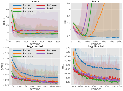
Fig. 7 studies the impact of SDE flow parameters on the and datasets by varying the flow time from 0.5 to 2.0. Note that according to the discussions in Section V-A, the flow step is accordingly increased to ensure the quality of SDE solver. The longer SDE flow time transforms the inputs to a more expressive posterior in order to reduce the gap to the exact posterior. As a result, the DLVKL-NSDE improves the performance with increasing on the dataset. As for the dataset, it is found that is enough since the longer flow time does not further improve the results. Note that the time complexity of DLVKL-NSDE increases with and . As a trade-off, we usually employ and in our experiments.

V-C Unsupervised learning on the dataset
It is notable that the proposed DLVKL-NSDE can also be used for unsupervised learning once we replace the input with the output in (18). To verify this, we apply the model to the handwritten digit dataset, which contains 60000 gray images with size . Since the VAE-type unsupervised learning structure requires feature transformations with varying dimensions, we employ the DLVKL-NSDE using and , i.e., the DLVKL. In this case, the DLVKL is similar to the GPLVM using back constraints (recognition model) [40]. The difference is that DLVKL uses instead of in GPLVM. Besides, the competitors include VAE [38] and DKL. The details of experimental configurations are provided in Appendix D.

Fig. 8 illustrates the two-dimensional latent space learned by different models, and several reconstructed digits. It is clearly observed that the models properly cluster the digits in the latent space. As for reconstruction, the three models reconstruct the profile of digits but lost some details due to the limited latent dimensionality. Besides, the reconstructed digits of DKL and DLVKL have slightly noisy background due to the Bayesian averaging and the share of kernel across 784 outputs. Finally, the DLVKL is found to have more reasonable reconstruction than DKL for some digits, e.g., digit “3”.
VI Conclusions
This paper proposes the DLVKL which inherits the advantages of DKL but provides better calibration through regularized latent representation. We further improve the DLVKL through (i) the NSDE transformation to yield expressive variational posterior, and (ii) the hybrid prior to achieve adjustable regularization on latent representation. We investigate the algorithmic characteristics of DLVKL-NSDE and compare it against existing deep GPs. The comparative results imply that the DLVKL-NSDE performs similarly to the well calibrated GP on small datasets, and shows superiority on large datasets.
Acknowledgments
This work was supported by the Fundamental Research Funds for the Central Universities (DUT19RC(3)070) at Dalian University of Technology, and it was partially supported by the Research and Innovation in Science and Technology Major Project of Liaoning Province (2019JH1-10100024), the National Key Research and Development Project (2016YFB0600104), and the MIIT Marine Welfare Project (Z135060009002).
Appendix A Viewing existing deep GPs in the framework of (3)
A-A Deterministic representation learning of
The DKL [26] has the transformation from to performed through a deterministic manner . As a result, the ELBO is expressed as
Different from (6), the purely deterministic transformation in the above ELBO will risk over-fitting, especially on small datasets, which has been verified in our numerical experiments.
A-B Bayesian representation learning of via GPs
Inspired by NN, the DGP [31] extends to a -layer hierarchical structure, wherein each layer is a sparse GP, as
where . As a result, the ELBO is expressed as
where . Due to the complete GP paradigm, the DGP naturally guards against over-fitting. But the capability of representation learning is limited by the finite inducing variables for massive data.
A-C Bayesian representation learning of via SDE
Different from traditional DGP, the sequence of transformation of which is indexed on discrete domain, the differential GP (DiffGP) [46] generalizes the transformation through the SDE indexed on continuous-time domain. Specifically, given the same dimension , , the posterior transformation through a sparse GP can be extended and interpreted as a SDE as
where is a diagonal matrix; and we have
In the above equations, and are the mean and covariance of the inducing variables shared across time. Thereafter, the ELBO over discrete time points for supervised learning is derived as
Different from (10), the sparse GP assisted SDE here results in analytical KL terms due to the Gaussian posteriors.
Appendix B -ELBO interpreted from VIB
We can interpret the DLVKL from the view of variational information bottleneck (VIB) [56]. Suppose that is a stochastic encoding of the input , our goal is to learn an encoding that is maximally informative about the output subject to a constraint on its complexity as
where represents the mutual information (MI) between two random variables. The above constraint is applied in order to learn a good representation rather than the simple identity . By introducing a Lagrange multiplier to the above problem, we have
As for the MI terms in , given the joint distribution , the MI is expressed as
where is the empirical distribution estimated from training data. Note that has no trainable parameters. Besides, the MI is
where .
Finally, we have the ELBO
which recovers the bound in (18) when we use sparse GP for and the NSDE transformation for .
Appendix C Proof of Proposition 1
Proof.
When the posterior collapse happens in the initial stage, we have (i) the zero KL staying at its local minimum; and (ii) the mapped inputs , and inducing inputs , . As a result, the relative distance between any two inputs always follow . We therefore have the collapsed kernel value
where , which is composed of the model parameters , is independent of inputs. This makes and be the matrices with all the elements being the same, which however are not invertible. In practice, we usually add a positive numeric jitter to the diagonal elements of and in order to relieve this issue.
When we are attempting to optimize the GP parameters, the collapsed kernel cannot measure the correlations among inputs. In this case, it is observed that the posterior mean for follows
where is the average of . It indicates that the GP degenerates to a constant predictor. For example, we know that the optimum of the mean of for GP regression satisfies [10]
When is normally normalized, i.e., , we have and therefore . As for classification, the degenerated constant predictor will simply use the percentages of training labels as class probabilities.
Hence, due to the constant prediction mean, what the optimizer can do is adjusting all the parameters of the encoder and GP for simply calibrating the prediction variances in order to fit the output variances in training data. ∎
Appendix D Experimental details
Toy cases. For the two toy cases, we adopt the settings for the following regression and classification tasks except that (i) the inducing size is ; (ii) the length-scales of the RBF kernel is initialized as 1.0; (iii) the batch size is ; and finally (iv) the Adam optimizer is ran over 5000 iterations.
Regression and classification tasks. The experimental configurations for the six regression tasks (, , -, , , ) and two classification tasks (-, ) are elaborated as below.
As for data preprocessing, we perform standardization over input dimensions to have zero mean and unit variance. Additionally, the outputs are standardized for regression. We shuffle the data and randomly select 10% for testing. The shuffle and split are repeated to have ten instances for multiple runs.
As for the GP part, we adopt the RBF kernel with the length-scales initialized as and the signal variance initialized as . The inducing size is . The related positions of inducing points are initialized in the original input space through clustering techniques and then passed through the SDE transformation as for DLVKL-NSDE. The variational parameters for the inducing variables are initialized as and . We set the prior parameter as on the small , and - datasets and on the remaining datasets, and have the SDE parameters as and .
As for the MLP part, we use the fully-connected (FC) NN with three hidden layers and the ReLU activation. The number of units for the hidden layers is . Particularly, the MLPs of DLVKL-NSDE in (15) share the hidden layers but have separate output layers for explaining the drift and diffusion, respectively. The diffusion variance is initialized as . Additionally, since the SDE flows over time, we include time as additional inputs for the MLPs. And all the layers except the output layers share the parameters over time.
As for the optimization, we employ the Adam with the batch size of 256, the learning rate of ,555The training of GPs with Adam often uses the learning rate of . While the training of NN often uses the learning rate of . Since the DLVKL-NSDE is a hybrid model, we adopt a medium learning rate of . and the maximum number of iterations as 3000 on the small , and - datasets, 100000 on the large dataset, and 20000 on the remaining datasets. In the experiments, we do not adopt additional fine-tune tricks, e.g., the scheduled learning rate, the regularized weights, or the dropout technique, for MLPs.
The - image classification task. For this image classification dataset, we build our codes upon the resnet-20 architecture implemented at https://github.com/yxlijun/cifar-tensorflow. We keep the convolution layers and the 64D FC layer, but additionally add the “FC(10+1)-tanh-FC(10+1)-tanh-FC(20)” layers plus the GP part for DLVKL-NSDE. For DKL, we drop the additional time input and use 10 units in the final layer. We use inducing points and directly initialize them in the latent space, since the encoded inducing strategy in the high-dimensional image space yields too many parameters which may make the model training difficult. We use the default data split, data augmentation and optimization strategies of resent-20 and run over 200 epochs.
The unsupervised learning task. For the dataset, the intensity of the gray images is normalized to . We build the decoder for the models using FC nets, the architecture of which is “784 Inputs-FC(196)-Relu-FC(49)-Relu-FC(22)”. Note that the DKL employs a deterministic encoder with the last layer as FC(2). The VAE uses a mirrored NN structure to build the corresponding decoder. Differently, the DKL and DLVKL adopt the sparse GP decoder for mapping the 2D latent inputs to 784 outputs using the shared RBF kernel with the length-scales initialized as and the signal variance initialized as . The inducing size is and the related positions are optimized through the encoded inducing strategy. The mean for the prior is obtained through the PCA transformation of . Finally, we employ the Adam optimizer with the batch size of 256, the learning rate of , and run it over 20000 iterations.
References
- [1] C. K. Williams and C. E. Rasmussen, Gaussian processes for machine learning. MIT press Cambridge, MA, 2006.
- [2] L. Wang and C. Li, “Spectrum-based kernel length estimation for Gaussian process classification,” IEEE Transactions on Cybernetics, vol. 44, no. 6, pp. 805–816, 2014.
- [3] P. Li and S. Chen, “Shared Gaussian process latent variable model for incomplete multiview clustering,” IEEE Transactions on Cybernetics, vol. 50, no. 1, pp. 61–73, 2020.
- [4] N. Lawrence, “Probabilistic non-linear principal component analysis with Gaussian process latent variable models,” Journal of Machine Learning Research, vol. 6, no. Nov, pp. 1783–1816, 2005.
- [5] R. Frigola, Y. Chen, and C. E. Rasmussen, “Variational Gaussian process state-space models,” in Advances in Neural Information Processing Systems, 2014, pp. 3680–3688.
- [6] H. Liu, J. Cai, and Y.-S. Ong, “Remarks on multi-output Gaussian process regression,” Knowledge-Based Systems, vol. 144, no. March, pp. 102–121, 2018.
- [7] B. Shahriari, K. Swersky, Z. Wang, R. P. Adams, and N. de Freitas, “Taking the human out of the loop: A review of Bayesian optimization,” Proceedings of the IEEE, vol. 104, no. 1, pp. 148–175, 2016.
- [8] J. Luo, A. Gupta, Y.-S. Ong, and Z. Wang, “Evolutionary optimization of expensive multiobjective problems with co-sub-pareto front Gaussian process surrogates,” IEEE Transactions on Cybernetics, vol. 49, no. 5, pp. 1708–1721, 2019.
- [9] E. Snelson and Z. Ghahramani, “Sparse gaussian processes using pseudo-inputs,” in Advances in Neural Information Processing Systems. MIT Press, 2006, pp. 1257–1264.
- [10] M. Titsias, “Variational learning of inducing variables in sparse Gaussian processes,” in Artificial Intelligence and Statistics, 2009, pp. 567–574.
- [11] D. P. Kingma and J. Ba, “Adam: A method for stochastic optimization,” arXiv preprint arXiv:1412.6980, 2014.
- [12] J. Hensman, N. Fusi, and N. D. Lawrence, “Gaussian processes for big data,” in Uncertainty in Artificial Intelligence. Citeseer, 2013, p. 282.
- [13] A. Wilson and H. Nickisch, “Kernel interpolation for scalable structured gaussian processes (kiss-gp),” in International Conference on Machine Learning. PMLR, 2015, pp. 1775–1784.
- [14] J. R. Gardner, G. Pleiss, R. Wu, K. Q. Weinberger, and A. G. Wilson, “Product kernel interpolation for scalable Gaussian processes,” in Artificial Intelligence and Statistics, 2018, pp. 1407–1416.
- [15] Y. Gal, M. van der Wilk, and C. Rasmussen, “Distributed variational inference in sparse Gaussian process regression and latent variable models,” in Advances in Neural Information Processing Systems, 2014, pp. 3257–3265.
- [16] H. Peng, S. Zhe, X. Zhang, and Y. Qi, “Asynchronous distributed variational gaussian process for regression,” in International Conference on Machine Learning. PMLR, 2017, pp. 2788–2797.
- [17] M. P. Deisenroth and J. W. Ng, “Distributed gaussian processes,” in International Conference on Machine Learning. PMLR, 2015, pp. 1481–1490.
- [18] H. Liu, J. Cai, Y. Wang, and Y.-S. Ong, “Generalized robust Bayesian committee machine for large-scale Gaussian process regression,” in International Conference on Machine Learning, 2018, pp. 1–10.
- [19] H. Liu, Y.-S. Ong, X. Shen, and J. Cai, “When Gaussian process meets big data: A review of scalable gps,” IEEE Transactions on Neural Networks and Learning Systems, pp. 1–19, 2020.
- [20] J. Lee, Y. Bahri, R. Novak, S. S. Schoenholz, J. Pennington, and J. Sohl-Dickstein, “Deep neural networks as Gaussian processes,” arXiv preprint arXiv:1711.00165, 2017.
- [21] Y. Cho and L. K. Saul, “Kernel methods for deep learning,” in Advances in Neural Information Processing Systems, 2009, pp. 342–350.
- [22] M. Hermans and B. Schrauwen, “Recurrent kernel machines: Computing with infinite echo state networks,” Neural Computation, vol. 24, no. 1, pp. 104–133, 2012.
- [23] D. K. Duvenaud, O. Rippel, R. P. Adams, and Z. Ghahramani, “Avoiding pathologies in very deep networks,” in Artificial Intelligence and Statistics, 2014, pp. 202–210.
- [24] R. M. Neal, Bayesian Learning for Neural Networks. Berlin, Heidelberg: Springer-Verlag, 1996.
- [25] A. G. d. G. Matthews, M. Rowland, J. Hron, R. E. Turner, and Z. Ghahramani, “Gaussian process behaviour in wide deep neural networks,” arXiv preprint arXiv:1804.11271, 2018.
- [26] A. G. Wilson, Z. Hu, R. Salakhutdinov, and E. P. Xing, “Deep kernel learning,” in Artificial Intelligence and Statistics, 2016, pp. 370–378.
- [27] A. G. Wilson, Z. Hu, R. R. Salakhutdinov, and E. P. Xing, “Stochastic variational deep kernel learning,” in Advances in Neural Information Processing Systems, 2016, pp. 2586–2594.
- [28] G.-L. Tran, E. V. Bonilla, J. P. Cunningham, P. Michiardi, and M. Filippone, “Calibrating deep convolutional Gaussian processes,” in Artificial Intelligence and Statistics, 2019, pp. 1554–1563.
- [29] N. Jean, S. M. Xie, and S. Ermon, “Semi-supervised deep kernel learning: Regression with unlabeled data by minimizing predictive variance,” in Advances in Neural Information Processing Systems, 2018, pp. 5322–5333.
- [30] M. Al-Shedivat, A. G. Wilson, Y. Saatchi, Z. Hu, and E. P. Xing, “Learning scalable deep kernels with recurrent structure,” Journal of Machine Learning Research, vol. 18, no. 1, pp. 2850–2886, 2017.
- [31] A. Damianou and N. Lawrence, “Deep Gaussian processes,” in Artificial Intelligence and Statistics, 2013, pp. 207–215.
- [32] H. Salimbeni and M. Deisenroth, “Doubly stochastic variational inference for deep Gaussian processes,” in Advances in Neural Information Processing Systems, 2017, pp. 4588–4599.
- [33] H.-C. Kim and Z. Ghahramani, “Bayesian gaussian process classification with the EM-EP algorithm,” IEEE Transactions on Pattern Analysis and Machine Intelligence, vol. 28, no. 12, pp. 1948–1959, 2006.
- [34] H. Nickisch and C. E. Rasmussen, “Approximations for binary Gaussian process classification,” Journal of Machine Learning Research, vol. 9, no. Oct, pp. 2035–2078, 2008.
- [35] A. C. Damianou, M. K. Titsias, and N. D. Lawrence, “Variational inference for latent variables and uncertain inputs in Gaussian processes,” Journal of Machine Learning Research, vol. 17, no. 1, pp. 1425–1486, 2016.
- [36] H. Liu, Y.-S. Ong, Z. Yu, J. Cai, and X. Shen, “Scalable Gaussian process classification with additive noise for various likelihoods,” arXiv preprint arXiv:1909.06541, 2019.
- [37] M. K. Titsias and N. D. Lawrence, “Bayesian Gaussian process latent variable model,” in International Conference on Artificial Intelligence and Statistics, vol. 9, 2010, pp. 844–851.
- [38] D. P. Kingma and M. Welling, “Auto-encoding variational bayes,” arXiv preprint arXiv:1312.6114, 2013.
- [39] S. R. Bowman, L. Vilnis, O. Vinyals, A. M. Dai, R. Jozefowicz, and S. Bengio, “Generating sentences from a continuous space,” arXiv preprint arXiv:1511.06349, 2015.
- [40] T. D. Bui and R. E. Turner, “Stochastic variational inference for Gaussian process latent variable models using back constraints,” in Black Box Learning and Inference NIPS workshop, 2015.
- [41] R. Friedrich, J. Peinke, M. Sahimi, and M. R. R. Tabar, “Approaching complexity by stochastic methods: From biological systems to turbulence,” Physics Reports, vol. 506, no. 5, pp. 87–162, 2011.
- [42] D. J. Rezende and S. Mohamed, “Variational inference with normalizing flows,” in International Conference on Machine Learning, 2015.
- [43] C. Chen, C. Li, L. Chen, W. Wang, Y. Pu, and L. C. Duke, “Continuous-time flows for efficient inference and density estimation,” in International Conference on Machine Learning, 2018, pp. 823–832.
- [44] R. T. Q. Chen, Y. Rubanova, J. Bettencourt, and D. K. Duvenaud, “Neural ordinary differential equations,” in Advances in Neural Information Processing Systems, S. Bengio, H. Wallach, H. Larochelle, K. Grauman, N. Cesa-Bianchi, and R. Garnett, Eds. Curran Associates, Inc., 2018, pp. 6571–6583.
- [45] X. Liu, T. Xiao, S. Si, Q. Cao, S. Kumar, and C.-J. Hsieh, “Neural SDE: Stabilizing neural ODE networks with stochastic noise,” arXiv preprint arXiv:1906.02355, 2019.
- [46] P. Hegde, M. Heinonen, H. Lähdesmäki, and S. Kaski, “Deep learning with differential Gaussian process flows,” in Artificial Intelligence and Statistics, 2019, pp. 1812–1821.
- [47] X. Chen, D. P. Kingma, T. Salimans, Y. Duan, P. Dhariwal, J. Schulman, I. Sutskever, and P. Abbeel, “Variational lossy autoencoder,” in International Conference on Learning Representations, 2017.
- [48] J. He, D. Spokoyny, G. Neubig, and T. Berg-Kirkpatrick, “Lagging inference networks and posterior collapse in variational autoencoders,” in International Conference on Learning Representations, 2019.
- [49] A. van den Oord, N. Kalchbrenner, O. Vinyals, L. Espeholt, A. Graves, and K. Kavukcuoglu, “Conditional image generation with PixelCNN decoders,” in Advances in Neural Information Processing Systems, 2016, pp. 4797–4805.
- [50] J. Tomczak and M. Welling, “Vae with a vampprior,” in Artificial Intelligence and Statistics, 2018, pp. 1214–1223.
- [51] K. He, X. Zhang, S. Ren, and J. Sun, “Deep residual learning for image recognition,” in IEEE Conference on Computer Vision and Pattern Recognition, 2016, pp. 770–778.
- [52] M. D. Hoffman, C. Riquelme, and M. J. Johnson, “The -VAE’s implicit prior,” in Workshop on Bayesian Deep Learning, NIPS, 2017, pp. 1–5.
- [53] I. Higgins, L. Matthey, A. Pal, C. Burgess, X. Glorot, M. Botvinick, S. Mohamed, and A. Lerchner, “beta-vae: Learning basic visual concepts with a constrained variational framework.” in International Conference on Learning Representations, 2017, pp. 1–6.
- [54] C. K. Sønderby, T. Raiko, L. Maaløe, S. K. Sønderby, and O. Winther, “How to train deep variational autoencoders and probabilistic ladder networks,” in International Conference on Machine Learning, 2016.
- [55] H. Fu, C. Li, X. Liu, J. Gao, A. Celikyilmaz, and L. Carin, “Cyclical annealing schedule: A simple approach to mitigating kl vanishing,” in The Association for Computational Linguistics: Human Language Technologies, 2019, pp. 240–250.
- [56] A. A. Alemi, I. Fischer, J. V. Dillon, and K. Murphy, “Deep variational information bottleneck,” arXiv preprint arXiv:1612.00410, 2016.
- [57] M. van der Wilk, C. E. Rasmussen, and J. Hensman, “Convolutional Gaussian processes,” in Advances in Neural Information Processing Systems, 2017, pp. 2845–2854.