Deep FBSDE Neural Networks for Solving Incompressible Navier-Stokes Equation and Cahn-Hilliard Equation
Abstract
Efficient algorithms for solving high-dimensional partial differential equations (PDEs) has been an exceedingly difficult task for a long time, due to the curse of dimensionality. We extend the forward-backward stochastic neural networks (FBSNNs) which depends on forward-backward stochastic differential equation (FBSDE) to solve incompressible Navier-Stokes equation. For Cahn-Hilliard equation, we derive a modified Cahn-Hilliard equation from a widely used stabilized scheme for original Cahn-Hilliard equation. This equation can be written as a continuous parabolic system, where FBSDE can be applied and the unknown solution is approximated by neural network. Also our method is successfully developed to Cahn-Hilliard-Navier-Stokes (CHNS) equation. The accuracy and stability of our methods are shown in many numerical experiments, specially in high dimension.
keywords:
forward-backward stochastic differential equation, neural network, Navier-Stokes, Cahn-Hilliard, high dimension1 Introduction
High-dimensional nonlinear partial differential equations (PDEs) are used widely in a number of areas of social and natural sciences. Due to the significant nonlinearity of nonlinear PDEs, particularly in high-dimensional cases, analytical solutions to nonlinear PDEs are typically difficult to acquire. Therefore, numerical solutions to these kinds of nonlinear PDEs are very important. However, due to their exponential increase in complexity, traditional approaches like finite difference method and finite element method fail in high-dimensional instances. Many fields pay close attention to developments in numerical algorithms for solving high-dimensional PDEs. There are several numerical methods for solving nonlinear high-dimensional partial differential equations here, such as Monte Carlo method[1, 2], lattice rule[3] and sparse grid method[4, 5], etc. They exhibit relative adaptability in addressing high-dimensional problems. However, they typically require substantial computational resources, especially in high-dimensional scenarios. Monte Carlo method often demands a large number of sample points, while lattice rule and sparse grid method may require finer grids or adaptive strategies. Moreover, their convergence rates are usually relatively slow, particularly in high-dimensional situations. Achieving the desired accuracy may entail a significant amount of computation.
Recently, deep neural networks (DNNs) have been used to create numerical algorithms which work well at overcoming the curse of dimensionality and successfully solving high-dimensional PDEs[6, 7, 8, 9, 10, 11, 12, 13, 14, 15, 16, 17, 18, 19, 20, 21, 22]. Inspired by Ritz method, deep Ritz method (DRM) [8] is proposed to solve variational problem arising from PDEs. The deep Galerkin method (DGM) is proposed in [18] to solve high-dimensional PDEs by approximating the solution with a deep neural network which is trained to satisfy the differential operator, initial condition, and boundary conditions.The physics-informed neural networks (PINN) is presented in [16], where the PDE is embedded into the neural network by utilizing automatic differentiation (AD). Three adaptive techniques to improve the computational performance of DNNs methods for high-dimensional PDEs are presented in [21]. The authors in [12] proposed an approach for scattering problems connected with linear PDEs of the Helmholtz type that relies on DNNs to describe the forward and inverse map. In [9], the deep backward stochastic differential equation (BSDE) method based on the nonlinear Feynman-Kac formula (see e.g.[23]) is proposed, which is used in [10] to estimate the solution of eigenvalue problems for semilinear second order differential operators.
The PINN and deep BSDE method are two different kinds of numerical frameworks for solving general PDEs. The AD is used to avoid truncation error and the numerical quadrature errors of variational form. Some gradient optimization methods are used to update the neural network so that the loss of the differential equation and boundary condition is reduced. The deep BSDE method treats the BSDE as a stochastic control problem with the gradient of the solution being the policy function and parameterizes the control process of the solution by DNNs. Then it trains the resulting sequence of networks in a global optimization given by the prescribed terminal condition. These methods do not rely on the training data provided by some external algorithms, which can be considered as unsupervised learning methods. One drawback of PINN is the high computational complexity of its loss function, which includes the differential operator in the PDE to be solved. On the other hand, the deep BSDE method does not require the computation of high order derivatives. Moreover, the loss function used by deep BSDE method involves only simple additive calculations, thereby deep BSDE method iterates faster. The deep BSDE method has made high-dimensional problems solvable, which allows us to solve high-dimensional semilinear PDEs in a reasonable amount of time. Recently, there are some works related to deep BSDE method, see [6, 7, 10, 24, 25, 26, 27, 28, 29, 30, 31, 32, 33, 34, 35, 36]. Based on the deep BSDE method, an improved method called FBSNNs is proposed in [6]. The method proceeds by approximating the unknown solution using a fully connected feedforward neural network (FNN) and obtains the required gradient vector by applying AD. However, because the nonlinear Feynman-Kac formula is involved in the reformulation procedure, FBSNNs can only handle some specific Cauchy problems without boundary conditions. Then, it is desirable to extend the FBSNNs to other kinds of PDEs and deal with the problems with boundary conditions.
The Navier-Stokes equation is an important equation in fluid dynamics and the Cahn-Hilliard equation is widely used in multi-phase problems. These equations are difficult to solve due to their complexity. There are many deep learning methods that have been applied to solve these equations in one or two dimensions (see e.g.[37, 38, 39, 40, 41, 42]). However, these methods fail due to excessive complexity when the dimension is more than three. We choose to introduce the FBSNNs presented in [6] to solve these equations. We convert the incompressible Navier-Stokes equations into FBSDEs and then employ FBSNNs to solve them in two or three dimension. We develop a suitable numerical method based on the reflection principle to deal with the Neumann boundary condition and handle the Dirichlet boundary condition using the method mentioned in [43]. We rewrite the Cahn-Hilliard equation into a system of parabolic equations by adding stable terms reasonably, then the numerical solution of the new system is obtained using the FBSNNs. However, when dealing with mixed boundary condition, the above method should be improved. We utilize an approach which is similar to the method for Dirichlet boundary case, meanwhile we add an extra error item to the final loss function for the Neumann boundary condition. The equation can also be solved for periodic boundary condition with techniques involved the periodicity. Therefore, we can naturally solve the CHNS equation which is a coupled system of Navier-Stokes and Cahn-Hilliard equations.
The rest of this article is organized as follows. In Section 2, we introduce FBSDEs, deep BSDE method and FBSNNs method briefly. In Section 3, we present the approach to solve incompressible Navier-Stokes equations with different boundary conditions. A methodology is proposed in Section 4 to solve Cahn-Hilliard equation with different boundary conditions. In Section 5, the method to solve CHNS system is developed. Numerical experiments are given in Section 6 to verify the effectiveness of our methods. Finally, conclusions and remarks are given in Section 7.
2 FBSDEs, deep BSDE method and FBSNNs
2.1 A brief introduction of FBSDEs
The FBSDEs where the randomness in the BSDE driven by a forward stochastic differential equation (SDE), is written in the general form
| (1) |
where is a d-dimensional Brownian motion, , , and are all deterministic mappings of time and space, with the fixed . We refer to as the according to the stochastic control terminology. In order to guarantee the existence of a unique solution pair adapted to the augmented natural filtration, the standard well-posedness assumptions of [23] are required. Indeed, considering the quasi-linear, parabolic terminal problem
| (2) |
with and is the second-order differential operator
| (3) |
the nonlinear Feynman-Kac formula indicates that the solution of (1) coincides almost exactly with the solution of (2) (cf., e.g., [23])
| (4) |
As a result, the BSDE formulation offers a stochastic representation to the synchronous solution of a parabolic problem and its gradient, which is a distinct advantage for numerous applications in stochastic control.
2.2 Deep BSDE method
Inorder to review the deep BSDE method proposed in [9], we consider the following FBSDEs
| (5) |
which is the integration form of (1). Given a partition of the time interval , the Euler-Maruyama scheme is used to discretize for and and we have
| (6) |
where , . The is approximated by a FNN with parameter for . The initial values and are treated as trainable parameters in the model. To make to approximate , the difference in the matching with a given terminal condition is used to define the expected loss function
| (7) |
which represents different realizations of the underlying Brownian motion, where the subscript corresponds to the -th realization of the underlying Brownian motion. The process is called the deep BSDE method.
2.3 FBSNNs
Raissi [6] introduced neural networks called FBSNNs to solve FBSDEs. The unknown solution is approximated by the FNN with the input and the required gradient vector is attained by applying AD. The parameter of FNN can be learned by minimizing the loss function given explicitly in equation (9) obtained from discretizing the FBSDEs (5) using the Euler-Maruyama scheme
| (8) |
where represents the estimated value of given by the FNN and is the reference value corresponding to , which is obtained from the calculation in (8). The loss function is then given by
| (9) |
where the subscripts is the same meaning as it in (7).
The deep BSDE method only calculates the value of . This means that in order to obtain an approximation to at a later time , we have to retrain the algorithm. Furthermore, the number of the FNNs grows with the number of time steps , which makes training difficult. In this article, we use the FBSNNs. The FNN is expected to be able to approximate over the entire computational area instead of only one point. That is, we will use multiple initial points to train the FNN. In order to improve the efficiency, the number of Brownian motion trajectories for each initial point is set as .
3 Deep neural network for solving the incompressible Navier-Stokes equation
3.1 A class of FBSDEs associated to the incompressible Navier-Stokes equation
The Cauchy problem for deterministic backward Navier–Stokes equation for the velocity field of the incompressible and viscous fluid is
| (10) |
which is obtained from the classical Navier–Stokes equation via the time-reversing transformation
| (11) |
Here represents the -dimensional velocity field of a fluid, is the pressure, is the viscosity coefficient, and stands for the external force. We now study the backward Navier–Stokes equation (10) in with different boundary conditions.
Then, the PDE (10) is associated through the nonlinear Feynman-Kac formula to the following FBSDEs
| (12) |
where
3.2 The algorithm for solving the incompressible Navier-Stokes equation
Given a partition of , we consider the Euler-Maruyama scheme with for FBSDEs (12)
| (13) |
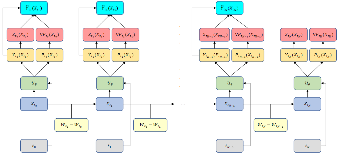
where and . The represents the estimated value of at time given by the FNN, respectively. The is the reference value of , which is obtained from the calculation in the second equation in (13). We utilize different initial sampling points for training the FNN. The algorithm of the proposed scheme is summarized in Algorithm 1. Illustration of the Algorithm 1 for solving the incompressible Navier-Stokes equation is shown in Figure 1.
| (14) | ||||
3.3 The algorithm for solving the incompressible Navier-Stokes equation with Dirichlet boundary condition
For the backward Navier–Stokes equation (10) in with the Dirichlet boundary condition
| (15) |
the corresponding FBSDEs can be rewritten as the following form according to [43] by the nonlinear Feynman-Kac formula
| (16) |
where , the stopping time be the first time that the process exits and
| (17) |
Through the Euler scheme, the discrete formulation of the FBSDEs (16) can be obtained accordingly
| (18) |
where . It should be noted that we will calculate the stop time after the iteration of is completed. Supposing when , we let on and update to satisfy (18). The algorithm of the proposed scheme is similar as Algorithm 1.
3.4 The algorithm for solving the incompressible Navier-Stokes equation with Neumann boundary condition
We consider the backward Navier–Stokes equation (10) with the Neumann boundary condition
| (19) |
where is the unit normal vector at pointing outward of . Supposing and , where and are symmetric to the boundary . Then we have
| (20) |
If , let , and if , let is the symmetric point of to the boundary . The is used to denote the intersection of the line segment and . Therefore, the discretization can be rewritten similarly as
| (21) |
where . The algorithm of the proposed scheme is similar as Algorithm 1.
Remark 1.
There are some similar works in [25, 29] for dealing with the Neumann boundary conditions. If during the iterative process, the authors [25, 29] choose to reflect on the boundary , which allows them to deal with the homogeneous Neumann conditions. In contrast, our method can deal with non-homogeneous Neumann boundary conditions.
4 Deep neural network for solving the Cahn-Hilliard equation
4.1 Rewrite Cahn-Hilliard equation into a parabolic PDE system
We consider the following Cahn-Hilliard equation, which has fourth order derivatives,
| (22) |
where is the unknown, e.g., the concentration of the fluid, is a function of , e.g.,the chemical potential, is the diffusion coefficient and is the model parameter. A first order stabilized scheme [44] for the Cahn-Hilliard equation (22) reads as
| (23) |
where is a suitable stabilized parameter. It is easy to derive the following equation
| (24) |
The first equation of (23) and (24) can be regarded as the discretization of the following modified Cahn-Hilliard equation in
| (25) |
where . By reversing the time and defining
the satisfies the following backward Cahn-Hilliard equation in
| (26) |
In order to satisfy the nonlinear Feynman-Kac formula and utilize the FBSNNs, we treat the backward Cahn-Hilliard equation (26) as a semilinear parabolic differential equation
| (27) |
with , and . Supposing and are two different eigenvalues of the coefficient matrix , then the coefficient matrix can be diagonalized by and so that , where is a matrix of eigenvectors. The system (27) becomes
| (28) |
where , and is chosen so that for , where .
Therefore, the system (28) is decomposed into two independent PDEs and the corresponding FBSDEs can be obtained as follows
| (29) |
where
and
The and are the forward stochastic processes corresponding to and respectively, which are constrained by at the initial time.
4.2 The algorithm for solving the Cahn-Hilliard equation
Given a partition of , we consider the simple Euler scheme for the FBSDEs (29) with
| (30) |
where and . The represents the estimated value of . The is the reference value of , which is obtained from the last two equations in (30).
The represents the estimated value of at time given by the FNN. Due to the diagonalization, we have
| (31) |
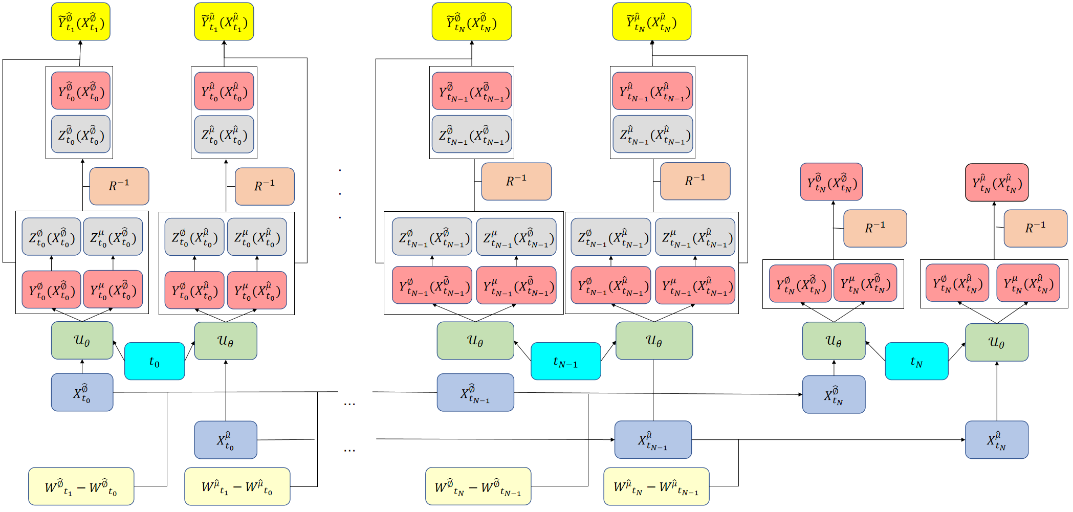
where subscript or is used to represent the -th or -th component of the vector. We utilize different initial sampling points for training the FNN. The algorithm of the proposed scheme is summarized as Algorithm 2. Illustration of the Algorithm 2 for solving the Cahn-Hilliard equation is shown in Figure 2.
| (32) | ||||
The Algorithm 2 shows that we only need to compute first-order derivatives during training, which causes the training time to increase linearly with the dimension . This makes our method capable of efficiently solving high-dimensional Cahn-Hilliard equations, which can be observed in the numerical experiments of solving the high-dimensional Cahn-Hilliard equations in Section 6.2.
4.3 The algorithm for solving the Cahn-Hilliard equation with mixed boundary condition
We consider the Cahn-Hilliard equation (22) in with the mixed condition
| (33) |
where is the unit normal vector at pointing outward of . The method described in Section 3.3 is used to deal with the Dirichlet boundary condition. For the Neumann boundary condition, it is noted that
| (34) |
where is given by the FNN with AD and subscript 2 represents the second component. Therefore, the method described in Section 3.4 can be used to deal with the Neumann boundary condition. It is shown in Section 6 that our method performs well numerically. The algorithm of the proposed scheme is similar as Algorithm 2.
4.4 The algorithm for solving the Cahn-Hilliard equation with periodic boundary condition
We consider the Cahn-Hilliard equation (22) with the periodic boundary condition,
| (35) |
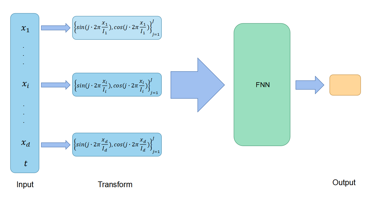
where is the period along the -th direction. To satisfy the condition (35), as in [10], we transform the input vector into a fixed trigonometric basis before applying the FNN. The component in is mapped as follows
| (36) |
where is the order of the trigonometric basis. The network structure for the periodic boundary condition (35) is shown in Figure 3. The algorithm of the proposed scheme is similar as Algorithm 2.
5 Deep neural network for solving Cahn-Hilliard-Navier-Stokes system
We now solve the coupled Cahn-Hilliard-Navier-Stokes equation in domain . According to Section 3.1 and Section 4.1, after time-reversing, the modified CHNS system is
| (37) |
where denotes a parameter, e.g., the strength of the capillary force comparing with the Newtonian fluid stress.
Similarly, we have the corresponding FBSDEs of (37) by diagonalizing and using the nonlinear Feynman-Kac formula
| (38) |
with and
The Euler scheme of (38) for is
| (39) |
where and . The , and represent the estimated values of , and , respectively. The , and are the reference values of , and , respectively, which are obtained from the last three equations in (39).
The represents the estimated value of at time given by the FNN . The represents the estimated value of at time given by the FNN . The calculations of and are based on (31). We choose different initial sampling points for training. The algorithm of the proposed scheme is summarized as Algorithm 3.
| (40) | ||||
6 Numerical experiments
In this section, we present a series of numerical results to validate our methods. For quantitative comparison, we calculate the error of the numerical solution and the exact solution in the relative norm and relative norm, which are defined as
The total number of training iterations is given by 1E+5, which is divided into 2E+4, 3E+4, 3E+4 and 2E+4 iterations with learning rates of 5E-3, 5E-4, 5E-5 and 5E-6, respectively, as the way in [6]. We employ the Adam optimizer to train FNNs. For each training step, we train the FNNs using 100 points randomly selected by the Latin hypercube sampling technique (LHS) in the domain. After the training process, we randomly pick 10000 points by the same method in the domain to test the FNNs. We set 4 hidden layers for the FNNs and each hidden layer consists of 30 neurons. The cosine function is taken as the activation function of the FNNs if we do not specify otherwise. In each numerical example, we use a set of the time interval , weights and the stabilization parameter . How to select or adjust these hyperparameters will be our future work. In our simulations, we use AMD Ryzen 7 3700X CPU and NVIDIA GTX 1660 SUPER GPU to train FNNs. The parameters and settings of numerical experiments are summarized in the Table 1.
| total number of training iterations | 1E+5 |
|---|---|
| number of iterations per segment | [2E+4, 3E+4, 3E+4, 2E+4] |
| learning rate per segment | [5E-3, 5E-4, 5E-5, 5E-6] |
| optimization algorithm | Adam |
| structure of neural networks | [30,30,30,30] |
| number of training points | 100 |
| number of test points | 10000 |
| point selection method | LHS |
| activation function | cos |
| CPU | AMD Ryzen 7 3700X |
| GPU | NVIDIA GTX 1660 SUPER |
6.1 Navier-Stokes equation
In this section, we numerically simulate the Taylor-Green vortex flow, which is a classical model to test numerical schemes for the incompressible Navier-Stokes equation. First, we consider the explicit 2D Taylor-Green vortex flow
| (41) |
for with constant and initial condition
| (42) |
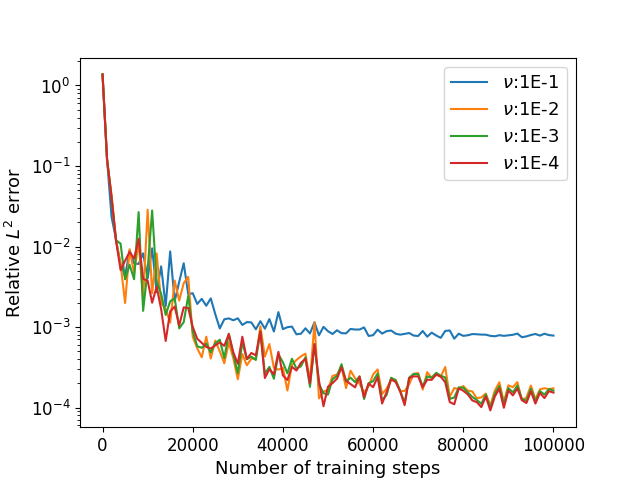
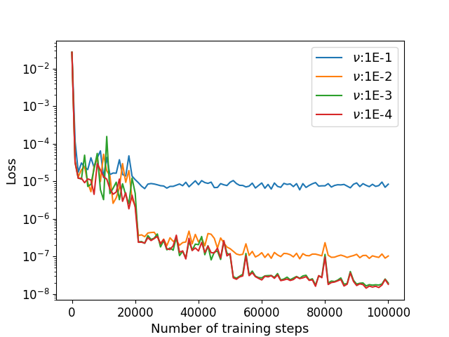
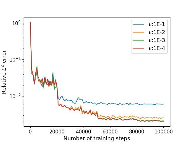
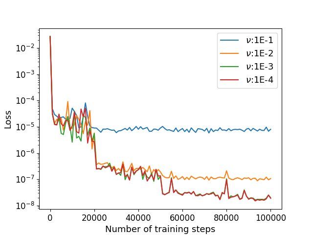
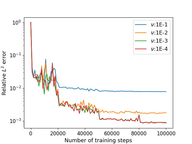
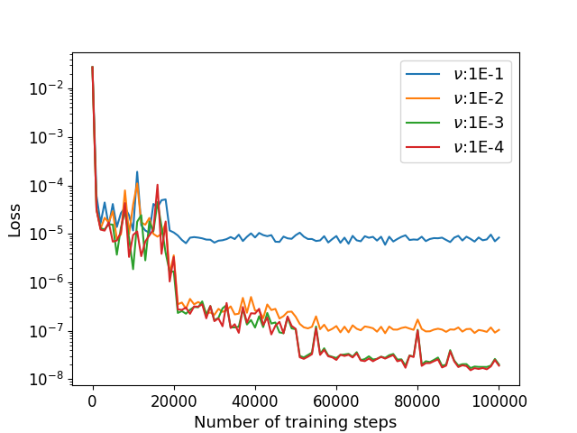
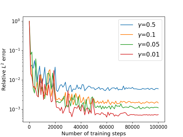
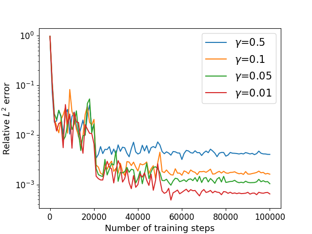
Algorithm 1 is employed to estimate with , , , and . The numerical results of the errors for and with different viscosity are shown in Table 2. The relative errors and the training losses with different training steps are shown in Figure 4. It is observed that these values decrease with parameter decreases. Similar phenomena will occur in the later experiments. Our method is not sensitive to the parameter . The training time is 500s for each case, which is a acceptable cost.
| 1E-1 | 1E-2 | 1E-3 | 1E-4 | |
| 1.60E-2 | 8.58E-3 | 7.41E-3 | 6.92E-3 | |
| 1.66E-2 | 5.72E-3 | 6.30E-3 | 6.45E-3 | |
| 7.23E-3 | 2.00E-3 | 9.02E-4 | 8.52E-4 | |
| 8.61E-3 | 1.39E-3 | 8.59E-4 | 8.36E-4 | |
| 1.12E-1 | 2.41E-2 | 9.45E-3 | 8.40E-3 | |
| time | 500s | |||
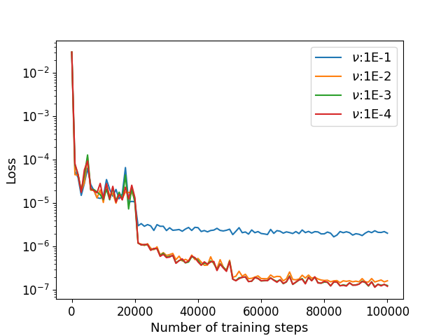
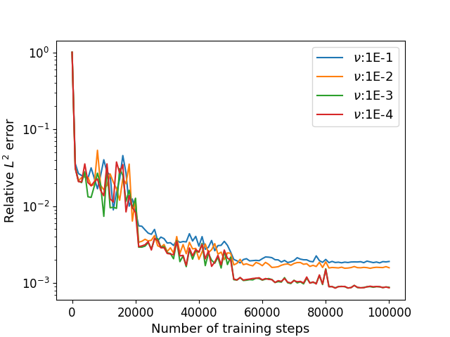
The 3D Arnold-Beltrami-Childress (ABC) flow is as follows
| (43) |
for with parameters , constant and initial condition
| (44) |
We estimate by applying the Algorithm 1 with parameters , , , , , . The numerical results of the errors for and with different viscosity are shown in Table 3. The relative errors and the training losses with different training steps are shown in Figure 5. The training time is 700s for each case, which is not too much longer than the 2D simulations.
| 1E-1 | 1E-2 | 1E-3 | 1E-4 | |
| 1.46E-2 | 8.77E-3 | 9.19E-3 | 9.16E-3 | |
| 1.41E-2 | 8.12E-3 | 9.34E-3 | 9.60E-3 | |
| 1.24E-2 | 9.32E-3 | 8.83E-3 | 8.81E-3 | |
| 6.20E-3 | 2.01E-3 | 1.81E-3 | 1.83E-3 | |
| 4.60E-3 | 2.36E-3 | 2.08E-3 | 2.05E-3 | |
| 7.05E-3 | 3.12E-3 | 2.38E-3 | 2.26E-3 | |
| 1.70E-1 | 6.92E-2 | 5.72E-2 | 5.58E-2 | |
| time | 700s | |||
Next, we consider the 2D Taylor-Green vortex flow (41)–(42) with the Dirichlet boundary condition (15) for . The other parameters remain the same as the first example. We use the algorithm in Section 3.3 and the numerical results of the errors for and with different viscosity parameters are shown in Table 4 and Figure 6 depicts the training processes. We also consider the 2D Taylor-Green vortex flow (41)–(42) with the Neumann boundary condition (19) for . We use the algorithm in Section 3.4 and the numerical results of the errors for and with different viscosity parameters are shown in Table 5 and the training processes are shown in Figure 7.
| 1E-1 | 1E-2 | 1E-3 | 1E-4 | |
| 4.96E-3 | 8.19E-3 | 7.13E-3 | 6.99E-3 | |
| 5.44E-3 | 5.70E-3 | 6.09E-3 | 6.41E-3 | |
| 1.89E-3 | 1.57E-3 | 8.90E-4 | 8.70E-4 | |
| 1.92E-3 | 1.59E-3 | 8.62E-4 | 8.57E-4 | |
| 3.26E-2 | 2.20E-2 | 9.28E-3 | 8.83E-3 | |
| time | 700s | |||
| 1E-1 | 1E-2 | 1E-3 | 1E-4 | |
| 1.50E-2 | 9.45E-3 | 7.65E-3 | 7.35E-3 | |
| 1.55E-2 | 6.10E-3 | 6.50E-3 | 6.64E-3 | |
| 8.05E-3 | 1.98E-3 | 9.27E-4 | 8.83E-4 | |
| 7.59E-3 | 1.52E-3 | 8.60E-4 | 8.53E-4 | |
| 1.11E-1 | 2.43E-2 | 9.36E-3 | 9.00E-3 | |
| time | 900s | |||
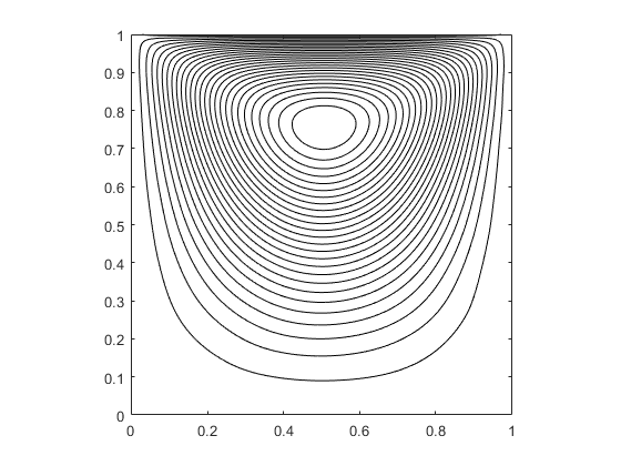
Now, we consider the 2D lid driven cavity flow for with the boundary and initial conditions
| (45) |
where represents the upper boundary. We utilize the algorithm in Section 3.3 to simulate . We impose boundary conditions to the network in the training process and let
| (46) |
where represents the estimate of output by the FNN. Therefore, it is easily verified that satisfies the boundary conditions of . For the condition of on , we add the following additional term to the loss function in Algorithm 1
| (47) |
where represents the -th point among the points selected on at time . The parameters are chosen as , , , , , , . To improve accuracy and save training time, we use the time adaptive approach II mentioned in [41]. At , the stream function and the pressure with are visually shown in Figure 8. These results are consistent with benchmark results.
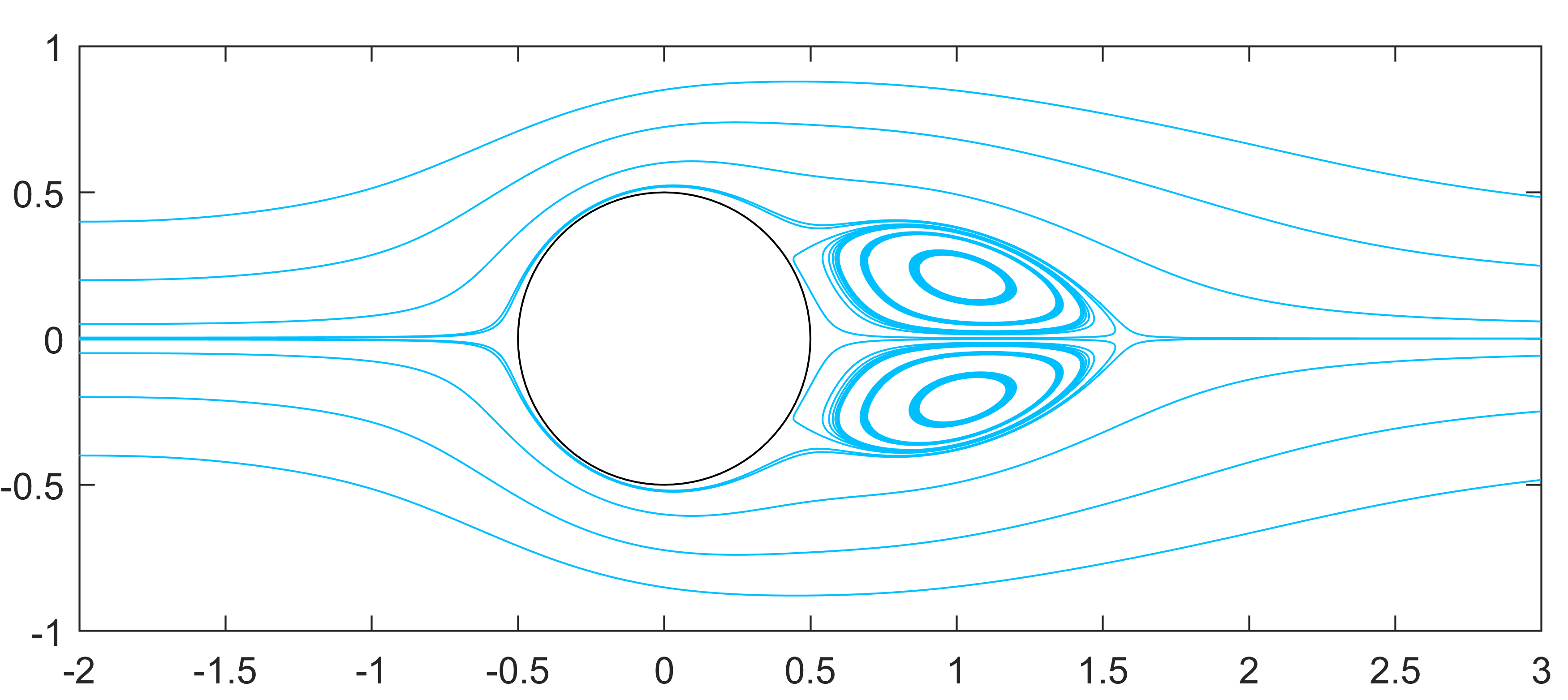
Finally, we consider that the flow past a circular obstacle for . The center of the obstacle is at position with the diameter . The boundary and initial conditions are given
| (48) |
where represent the upper, lower, left, right boundaries and the surface of the obstacle. The is the inlet velocity and is the unit normal vector at pointing outward of . We utilize the algorithm in Section 3.3 to deal with the Dirichlet boundary conditions on , while we utilize the algorithm in Section 3.4 to deal with the condition on . We let
| (49) |
where represents the estimate of output by the FNN. Therefore, it is easily verified that satisfies the boundary conditions of . For the conditions of on and on , we add the following additional term to the loss function in Algorithm 1
| (50) |
where denotes the -th point among the points selected on at time and denotes the -th point among the points selected on at time . The parameters are chosen as , , , , , , and . Similarly, We choose to use the time adaptive approach II mentioned in [41] to improve accuracy and save training time. At , the streamline is shown in Figure 9 with , which is consistent with the result obtained by traditional numerical methods.
6.2 Cahn-Hilliard equation
In this section, we consider the Cahn-Hilliard equation (22) in with initial condition
| (51) |
The exact solution is given by
| (52) |
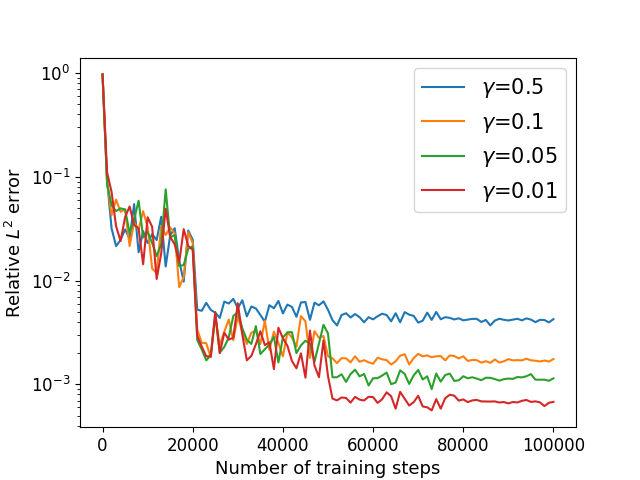
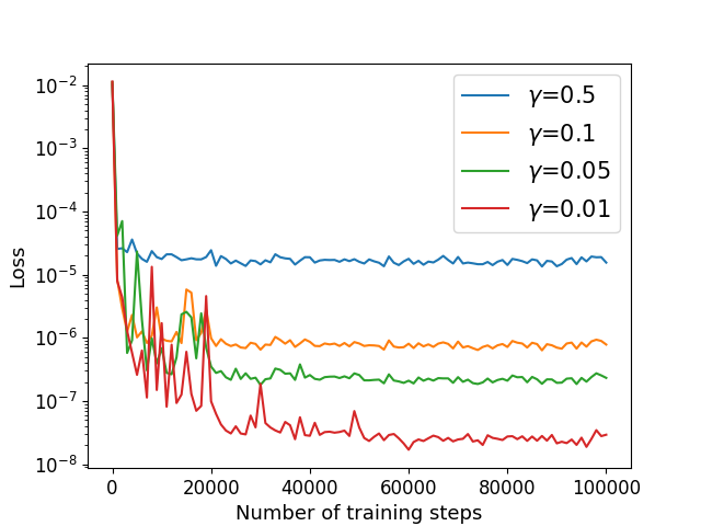
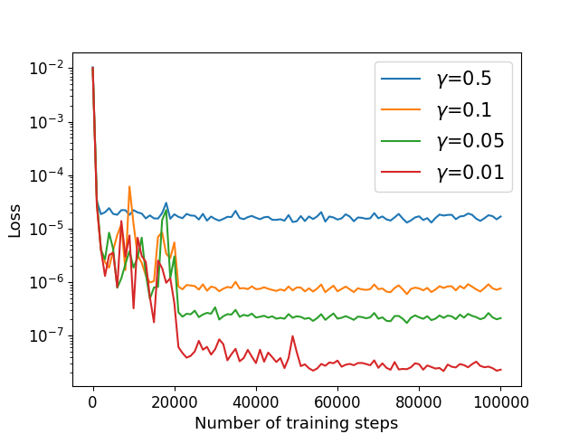
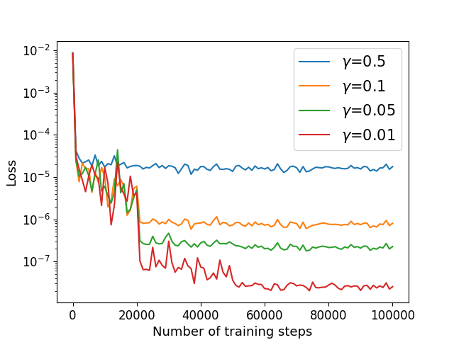
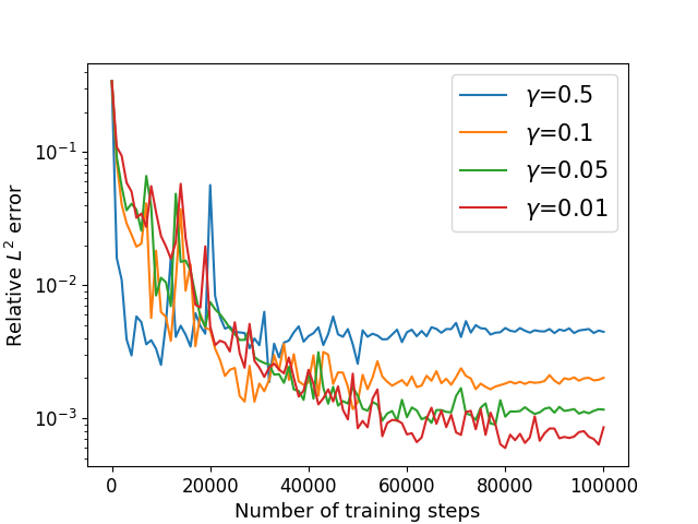
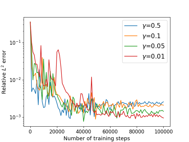
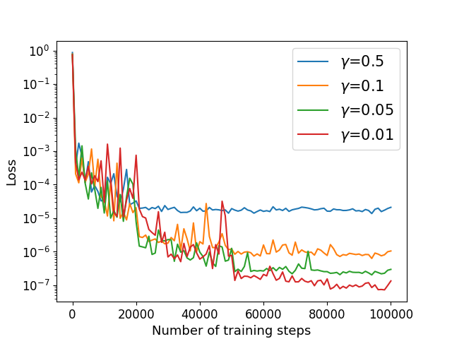
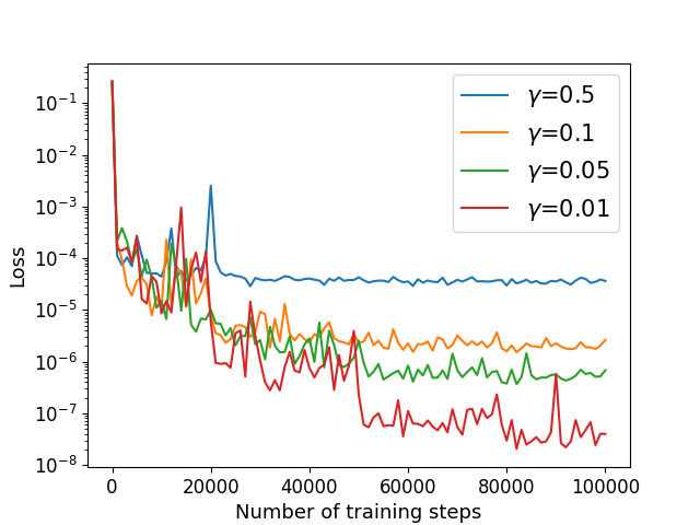
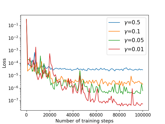
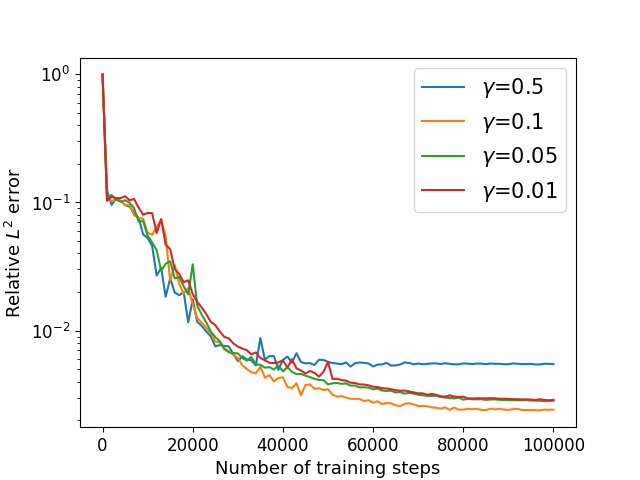
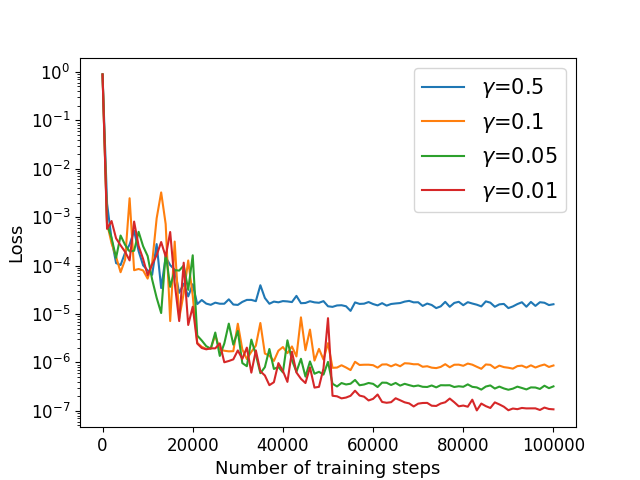
The parameters are taken as 5E-4, , , and . We estimate using Algorithm 2 with different parameter in different dimension. The numerical results of the errors for with different and are recorded in Table 6. Training processes in different dimension are shown in Figure 10. For a fixed dimension, when decreases, the relative error and training losses decrease. Our method is not sensitive to parameters and , and the training time of our method increases linearly with the dimension , while the accuracy does not decrease. It works for the problem with high-order derivatives in high dimensions, which does not make the training difficult.
| d | S | time | |||
|---|---|---|---|---|---|
| 2 | 0.5 | 0.5 | 3.25E-2 | 5.02E-3 | 1200s |
| 0.1 | 0.1 | 2.56E-3 | 1.67E-3 | ||
| 0.05 | 0.05 | 2.08E-3 | 1.13E-3 | ||
| 0.01 | 0.01 | 1.99E-3 | 6.67E-4 | ||
| 50 | 0.5 | 0.5 | 1.08E-2 | 4.06E-3 | 3200s |
| 0.1 | 0.1 | 3.78E-3 | 1.65E-3 | ||
| 0.05 | 0.05 | 3.48E-3 | 1.04E-3 | ||
| 0.01 | 0.01 | 3.63E-3 | 6.49E-4 | ||
| 100 | 0.5 | 0.5 | 1.62E-2 | 4.25E-3 | 5200s |
| 0.1 | 0.1 | 6.46E-3 | 1.76E-3 | ||
| 0.05 | 0.05 | 2.38E-3 | 1.15E-3 | ||
| 0.01 | 0.01 | 4.06E-3 | 6.79E-4 |
We consider the Cahn-Hilliard equation (22) with exact solution (52) defined in satisfying the mixed boundary conditions (33) on , where and are given by the exact solution. In this case, we choose . We utilize the algorithm in Section 4.3 to solve with different parameter in different dimension. The numerical results of the errors for with different and are recorded in Table 7 and the training processes are shown in Figure 11. Our method works for boundary value problem in high dimension.
| d | S | time | |||
|---|---|---|---|---|---|
| 2 | 0.5 | 0.5 | 1.69E-2 | 6.12E-3 | 1800s |
| 0.1 | 0.1 | 4.52E-3 | 1.94E-3 | ||
| 0.05 | 0.05 | 3.64E-3 | 1.69E-3 | ||
| 0.01 | 0.01 | 3.72E-3 | 1.92E-3 | ||
| 50 | 0.5 | 0.5 | 2.40E-2 | 4.46E-3 | 3800s |
| 0.1 | 0.1 | 1.13E-2 | 2.01E-3 | ||
| 0.05 | 0.05 | 5.77E-3 | 1.16E-3 | ||
| 0.01 | 0.01 | 7.33E-3 | 8.55E-4 | ||
| 100 | 0.5 | 0.5 | 1.14E-2 | 2.58E-3 | 6000s |
| 0.1 | 0.1 | 9.52E-3 | 2.10E-3 | ||
| 0.05 | 0.05 | 1.10E-2 | 1.44E-3 | ||
| 0.01 | 0.01 | 4.98E-2 | 9.56E-4 |

Next, we consider the Cahn-Hilliard equation (22) with exact solution (52) defined in with the periodic boundary condition (35) and mixed boundary condition (33) on , where the periods , where and are given by the exact solution. We choose and other parameters remain the same as previous example. We utilize the algorithm in Sections 4.3 and 4.4 to solve with different parameter . The numerical results of the errors for are recorded in Table 8 and Figure 12.
| S | time | |||
|---|---|---|---|---|
| 0.5 | 0.5 | 9.98E-3 | 5.48E-3 | 3400s |
| 0.1 | 0.1 | 4.86E-3 | 2.42E-3 | |
| 0.05 | 0.05 | 7.86E-3 | 2.84E-3 | |
| 0.01 | 0.01 | 7.39E-3 | 2.88E-3 |
6.3 Cahn-Hilliard-Navier-Stokes equation
In this section, we consider the coupled CHNS system
| (53) |
for with the constant and initial condition
| (54) |
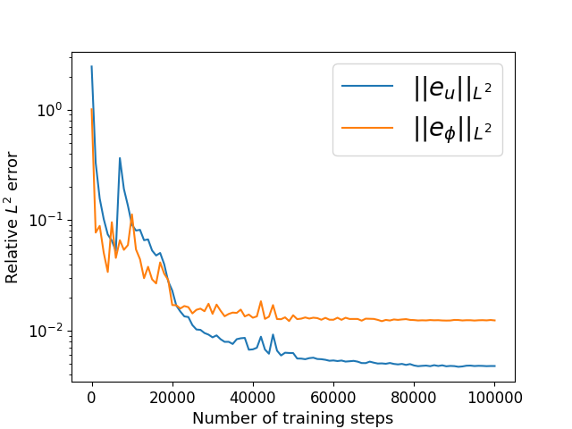
The parameters are taken as , , , , , , , , . The numerical results of the errors for , and are recorded in Table 9 and Figure 13 shows the training process, where the Algorithm 3 in Section 5 is implemented. It is easy to see that our method works for the coupled system.
| time | |||||||
|---|---|---|---|---|---|---|---|
| 2.41E-2 | 2.30E-2 | 1.25E-2 | 1.31E-2 | 1.16E-2 | 4.78E-3 | 2.07E-1 | 1800s |
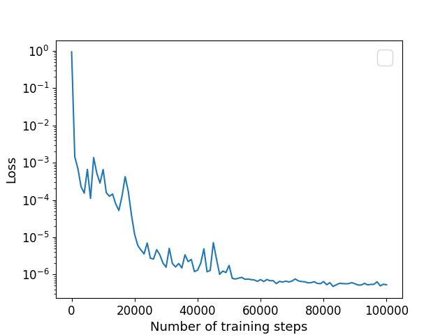
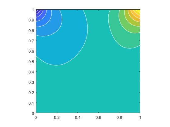
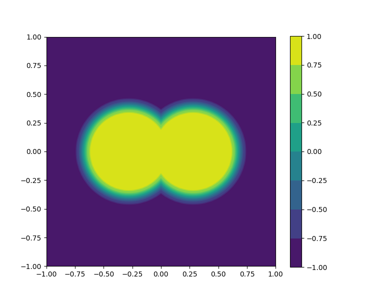
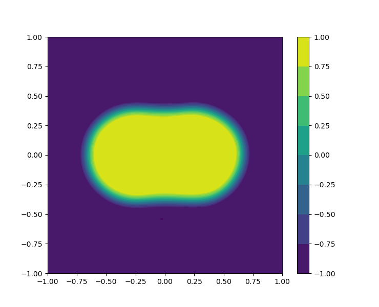
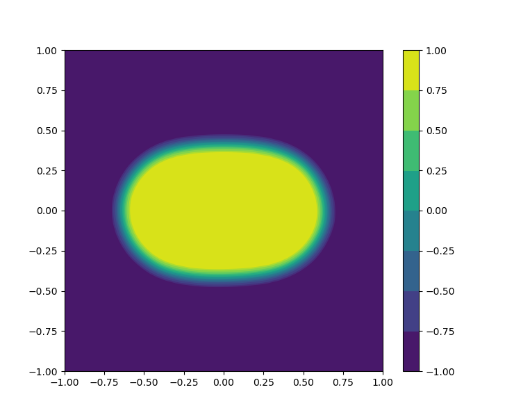
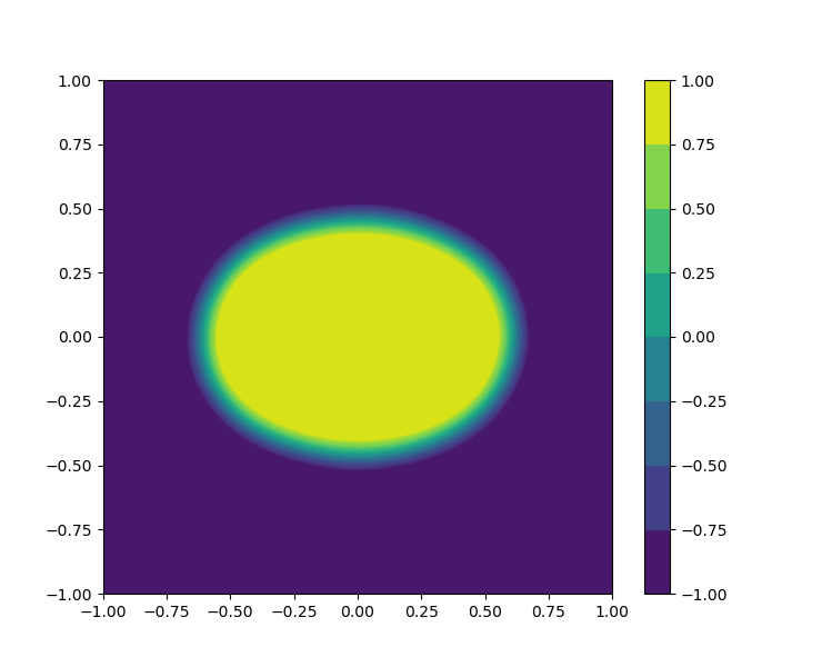
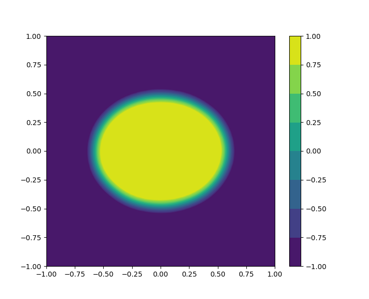
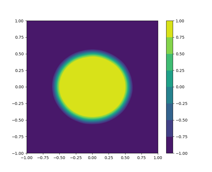
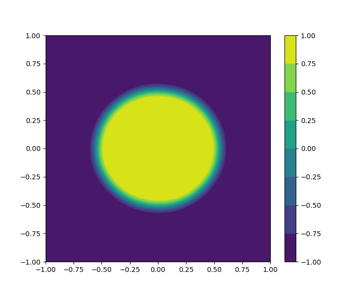
Finally, we study the interface problem modeled by the CHNS system. In this example, we choose the square domain and the parameters , , , , , , , , . The initial conditions for and is given
| (55) |
where , , and . The time adaptive approach II in [41] is employed to reduce the training time. According to the conservation of mass, we add the following loss term to the final loss function defined in Algorithm 3
| (56) |
The cosine and tanh functions are chosen as activation functions for the FNNs and , respectively. The evolution of the bubbles merging is visually shown in Figure 14, which is coincide with the result in the literature.

7 Conclusions and remarks
In this article, we have presented the methods to obtain the numerical solutions of the incompressible Navier-Stokes equation, the Cahn-Hilliard equation and the CHNS system with different boundary conditions based on the Forward-Backward Stochastic Neural Networks. In particular, we utilize the modified Cahn-Hilliard equation that is derived from a widely used stabilized scheme for original Cahn-Hilliard, which can be diagonalized into a parabolic system. The FBSNNs are applied to this system, which works well for high-dimensional problem. We demonstrate the performance of our algorithms on a variety of numerical experiments. In all numerical results, our methods are shown to be both stable and accurate. In the future work, we will study on how to make the training more efficiently and provide the theoretical analysis for our methods with some assumptions.
Declarations
-
1.
–Ethical Approval
Not Applicable -
2.
–Availability of supporting data
The datasets generated during and/or analysed during the current study are available from the corresponding author on reasonable request. -
3.
–Competing interests
The authors have no relevant financial or non-financial interests to disclose. -
4.
–Funding
This research is partially supported by the National key R & D Program of China (No.2022YFE03040002) and the National Natural Science Foundation of China ( No.12371434). -
5.
–Authors’ contributions
All authors contribute to the study conception and design. Numerical simulations are performed by Deng Yangtao. All authors read and approve the final manuscript. -
6.
–Acknowledgments
This research is partially supported by the National key R & D Program of China (No.2022YFE03040002) and the National Natural Science Foundation of China ( No.12371434).
References
- [1] N. Kantas, A. Beskos, A. Jasra, Sequential Monte Carlo methods for high-dimensional inverse problems: A case study for the Navier–Stokes equations, SIAM/ASA Journal on Uncertainty Quantification 2 (1) (2014) 464–489.
- [2] X. Warin, Nesting Monte Carlo for high-dimensional non-linear PDEs, Monte Carlo Methods and Applications 24 (4) (2018) 225–247.
- [3] J. Dick, F. Y. Kuo, I. H. Sloan, High-dimensional integration: the quasi-Monte Carlo way, Acta Numerica 22 (2013) 133–288.
- [4] J. Shen, H. Yu, Efficient spectral sparse grid methods and applications to high-dimensional elliptic problems, SIAM Journal on Scientific Computing 32 (6) (2010) 3228–3250.
- [5] Z. Wang, Q. Tang, W. Guo, Y. Cheng, Sparse grid discontinuous Galerkin methods for high-dimensional elliptic equations, Journal of Computational Physics 314 (2016) 244–263.
- [6] M. Raissi, Forward–backward stochastic neural networks: deep learning of high-dimensional partial differential equations, in: Peter Carr Gedenkschrift: Research Advances in Mathematical Finance, World Scientific, 2024, pp. 637–655.
- [7] C. Beck, S. Becker, P. Cheridito, A. Jentzen, A. Neufeld, Deep splitting method for parabolic PDEs, SIAM Journal on Scientific Computing 43 (5) (2021) A3135–A3154.
- [8] W. E, B. Yu, The deep Ritz method: a deep learning-based numerical algorithm for solving variational problems, Communications in Mathematics and Statistics 6 (1) (2018) 1–12.
- [9] J. Han, A. Jentzen, W. E, Solving high-dimensional partial differential equations using deep learning, Proceedings of the National Academy of Sciences 115 (34) (2018) 8505–8510.
- [10] J. Han, J. Lu, M. Zhou, Solving high-dimensional eigenvalue problems using deep neural networks: A diffusion Monte Carlo like approach, Journal of Computational Physics 423 (2020) 109792.
- [11] Y. Khoo, J. Lu, L. Ying, Solving parametric PDE problems with artificial neural networks, European Journal of Applied Mathematics 32 (3) (2021) 421–435.
- [12] Y. Khoo, L. Ying, SwitchNet: a neural network model for forward and inverse scattering problems, SIAM Journal on Scientific Computing 41 (5) (2019) A3182–A3201.
- [13] L. Lu, X. Meng, Z. Mao, G. E. Karniadakis, DeepXDE: A deep learning library for solving differential equations, SIAM Review 63 (1) (2021) 208–228.
- [14] K. O. Lye, S. Mishra, D. Ray, P. Chandrashekar, Iterative surrogate model optimization (ISMO): an active learning algorithm for PDE constrained optimization with deep neural networks, Computer Methods in Applied Mechanics and Engineering 374 (2021) 113575.
- [15] L. Lyu, Z. Zhang, M. Chen, J. Chen, MIM: A deep mixed residual method for solving high-order partial differential equations, Journal of Computational Physics 452 (2022) 110930.
- [16] M. Raissi, P. Perdikaris, G. E. Karniadakis, Physics-informed neural networks: A deep learning framework for solving forward and inverse problems involving nonlinear partial differential equations, Journal of Computational physics 378 (2019) 686–707.
- [17] E. Samaniego, C. Anitescu, S. Goswami, V. M. Nguyen-Thanh, H. Guo, K. Hamdia, X. Zhuang, T. Rabczuk, An energy approach to the solution of partial differential equations in computational mechanics via machine learning: Concepts, implementation and applications, Computer Methods in Applied Mechanics and Engineering 362 (2020) 112790.
- [18] J. Sirignano, K. Spiliopoulos, DGM: A deep learning algorithm for solving partial differential equations, Journal of computational physics 375 (2018) 1339–1364.
- [19] Z. Wang, Z. Zhang, A mesh-free method for interface problems using the deep learning approach, Journal of Computational Physics 400 (2020) 108963.
- [20] Y. Zang, G. Bao, X. Ye, H. Zhou, Weak adversarial networks for high-dimensional partial differential equations, Journal of Computational Physics 411 (2020) 109409.
- [21] S. Zeng, Z. Zhang, Q. Zou, Adaptive deep neural networks methods for high-dimensional partial differential equations, Journal of Computational Physics 463 (2022) 111232.
- [22] Y. Zhu, N. Zabaras, P.-S. Koutsourelakis, P. Perdikaris, Physics-constrained deep learning for high-dimensional surrogate modeling and uncertainty quantification without labeled data, Journal of Computational Physics 394 (2019) 56–81.
- [23] E. Pardoux, S. Peng, Backward stochastic differential equations and quasilinear parabolic partial differential equations, in: B. L. Rozovskii, R. B. Sowers (Eds.), Stochastic partial differential equations and their applications, Springer, Berlin, Heidelberg, 1992, pp. 200–217.
- [24] C. Beck, S. Becker, P. Grohs, N. Jaafari, A. Jentzen, Solving the Kolmogorov pde by means of deep learning, Journal of Scientific Computing 88 (2021) 1–28.
- [25] V. Boussange, S. Becker, A. Jentzen, B. Kuckuck, L. Pellissier, Deep learning approximations for non-local nonlinear PDEs with Neumann boundary conditions, Partial Differential Equations and Applications 4 (6) (2023) 51.
- [26] Q. Chan-Wai-Nam, J. Mikael, X. Warin, Machine learning for semi linear PDEs, Journal of scientific computing 79 (3) (2019) 1667–1712.
- [27] Q. Feng, M. Luo, Z. Zhang, Deep signature FBSDE algorithm, Numerical Algebra, Control and Optimization 13 (3&4) (2023) 500–522.
- [28] M. Fujii, A. Takahashi, M. Takahashi, Asymptotic expansion as prior knowledge in deep learning method for high dimensional BSDEs, Asia-Pacific Financial Markets 26 (3) (2019) 391–408.
- [29] J. Han, M. Nica, A. R. Stinchcombe, A derivative-free method for solving elliptic partial differential equations with deep neural networks, Journal of Computational Physics 419 (2020) 109672.
- [30] J. Y. Nguwi, G. Penent, N. Privault, A deep branching solver for fully nonlinear partial differential equations, Journal of Computational Physics 499 (2024) 112712.
- [31] N. Nüsken, L. Richter, Interpolating between BSDEs and PINNs: deep learning for elliptic and parabolic boundary value problems, Journal of Machine Learning 2 (1) (2023) 31–64.
- [32] N. Nüsken, L. Richter, Solving high-dimensional Hamilton–Jacobi–Bellman PDEs using neural networks: perspectives from the theory of controlled diffusions and measures on path space, Partial Differential Equations and Applications 2 (4) (2021) 1–48.
- [33] H. Pham, X. Warin, M. Germain, Neural networks-based backward scheme for fully nonlinear PDEs, SN Partial Differential Equations and Applications 2 (1) (2021) 1–24.
- [34] A. Takahashi, Y. Tsuchida, T. Yamada, A new efficient approximation scheme for solving high-dimensional semilinear PDEs: control variate method for Deep BSDE solver, Journal of Computational Physics 454 (2022) 110956.
- [35] M. Sabate Vidales, D. Šiška, L. Szpruch, Unbiased deep solvers for linear parametric PDEs, Applied Mathematical Finance 28 (4) (2021) 299–329.
- [36] Y. Wang, Y.-H. Ni, Deep BSDE-ML learning and its application to model-free optimal control, arXiv preprint arXiv:2201.01318.
- [37] R. Mattey, S. Ghosh, A novel sequential method to train physics informed neural networks for Allen Cahn and Cahn Hilliard equations, Computer Methods in Applied Mechanics and Engineering 390 (2022) 114474.
- [38] T. P. Miyanawala, R. K. Jaiman, An efficient deep learning technique for the Navier-Stokes equations: Application to unsteady wake flow dynamics, arXiv preprint arXiv:1710.09099.
- [39] A. T. Mohan, D. V. Gaitonde, A deep learning based approach to reduced order modeling for turbulent flow control using LSTM neural networks, arXiv preprint arXiv:1804.09269.
- [40] M. Raissi, A. Yazdani, G. E. Karniadakis, Hidden fluid mechanics: A Navier-Stokes informed deep learning framework for assimilating flow visualization data, arXiv preprint arXiv:1808.04327.
- [41] C. L. Zhao, Solving Allen-Cahn and Cahn-Hilliard Equations using the Adaptive Physics Informed Neural Networks, Communications in Computational Physics 29 (3).
- [42] J. Yang, Q. Zhu, A Local Deep Learning Method for Solving High Order Partial Differential Equations., Numerical Mathematics: Theory, Methods & Applications 15 (1).
- [43] É. Pardoux, Backward stochastic differential equations and viscosity solutions of systems of semilinear parabolic and elliptic PDEs of second order, in: L. Decreusefond, B. Øksendal, J. Gjerde, A. S. Üstünel (Eds.), Stochastic Analysis and Related Topics VI, Springer, Boston, MA, 1998, pp. 79–127.
- [44] J. Shen, X. Yang, Numerical approximations of Allen-Cahn and Cahn-Hilliard equations, Discrete & Continuous Dynamical Systems 28 (4) (2010) 1669.