Deep Equilibrium Multimodal Fusion

Our DEQ fusion is particularly built on deep equilibrium models to recursively capture intra- and inter-modality interactions for multimodal fusion. The traditional deep neural networks have finite depth and perform the backward pass through every layer. Two interesting observations are that the hidden layers tend to converge to some fixed points, and employing the same weight in each layer of the network, so-called weight tying, still achieves competitive results. That leads to the design principles of deep equilibrium models and the goal is to simulate an infinite depth weight-tied deep network, producing high-level and stable feature representations.

Formally, the standard DEQ [6] is formulated as a weight-tied network, and such a network with parameter $\theta$ and a depth of $L$ computes a hidden state $\mathbf{z}$ as

$$\mathbf{z}^{[j+1]}=f_{\theta}(\mathbf{z}^{[j]};\mathbf{x}),\quad j=0,\dots,L-1$$

(1)

where the untransformed input $\mathbf{x}$ is injected at each layer, $\mathbf{z}^{[j]}$ is the hidden state at layer $j$ and $\mathbf{z}^{[0]}=\mathbf{0}$. As claimed in [6], the core idea of DEQ is that when there are infinite layers ($L\rightarrow\infty$), the system tends to converge to an equilibrium state $\mathbf{z}^{*}$ such that

$$\mathbf{z}^{*}=f_{\theta}(\mathbf{z}^{*};\mathbf{x}).$$

(2)

In practice, naively computing the equilibrium state requires excessive runtime. One convergence acceleration is to formulate Eq. 2 into a root-finding problem:

$$g_{\theta}(\mathbf{z};\mathbf{x})=f_{\theta}(\mathbf{z};\mathbf{x})-\mathbf{z}.$$

(3)

Some root solvers can then be applied to the residual $g_{\theta}$ to find the equilibrium state

$$\mathbf{z}^{*}=\mathrm{RootSolver}(g_{\theta};\mathbf{x}).$$

(4)

Instead of backpropagating through each layer, we can compute gradients analytically as

$$\frac{\partial\ell}{\partial(\cdot)}=\frac{\partial\ell}{\partial\mathbf{z}^{*}}\left(\left.{-J_{g_{\theta}}^{-1}}\right|_{\mathbf{z}^{*}}\right)\frac{\partial f_{\theta}(\mathbf{z};\mathbf{x})}{\partial(\cdot)},$$

(5)

where $\ell=\mathcal{L}(\mathbf{z}^{*},\mathbf{y})$ is a loss between $\mathbf{z}^{*}$ and the target $\mathbf{y}$, $\left.{J_{g_{\theta}}^{-1}}\right|_{\mathbf{z}^{*}}$ is the inverse Jacobian of $g_{\theta}$ at $\mathbf{z}^{*}$. As it is expensive to compute the inverse Jacobian term, [6] proposed to alternatively solve a linear system by involving a vector-Jacobian product

$$\mathbf{x}\left(\left.{J_{g_{\theta}}}\right|_{\mathbf{z}^{*}}\right)+\frac{\partial\ell}{\partial\mathbf{z}^{*}}=\mathbf{0}.$$

(6)

With the formulation above, DEQ represents an infinite depth network with just one layer $f_{\theta}$, which converges to an equilibrium state, and can be backpropagated implicitly with a single computation.

Next, we formulate our DEQ fusion method. Given a set of unimodal features $\mathbf{x}=\{\mathbf{x}_{1},\mathbf{x}_{2},\dots,\mathbf{x}_{N}\}$ from $N$ modalities, our goal is to find a unified feature that integrates the information from all modalities. To ensure the informativeness of our final integrated feature, we first execute another nonlinear projection $f_{\theta_{i}}(\cdot)$ to extract higher-level information within each modality:

$$\mathbf{z}_{i}^{[j+1]}=f_{\theta_{i}}(\mathbf{z}_{i}^{[j]};\mathbf{x}_{i}),$$

(7)

where $\mathbf{z}_{i}^{[j]}$ is the $j$-th output of the layer for modality $i$ and $\mathbf{z}_{i}^{[0]}$ is initialized to $\mathbf{0}$. $\mathbf{x}_{i}$ is the injected input feature for modality $i$. Our fusion design is flexible from the standpoint that $f_{\theta_{i}}(\cdot)$ can be altered arbitrarily to fit multiple modalities. In our case, $f_{\theta_{i}}(\cdot)$ is designed to be similar to a simple residual block [18]. Following [7], we adopt group normalization [62] instead of batch normalization [22] for stability. Hence, $f_{\theta_{i}}(\cdot)$ is formulated as

$$\begin{gathered}\hat{\mathbf{z}}_{i}^{[j]}=\mathrm{ReLU}\left(\mathrm{GroupNorm}\left(\hat{\theta}_{i}\mathbf{z}_{i}^{[j]}+\hat{\mathbf{b}}_{i}\right)\right)\\ \tilde{\mathbf{z}}_{i}^{[j]}=\mathrm{GroupNorm}\left(\tilde{\theta}_{i}\hat{\mathbf{z}}_{i}^{[j]}+\mathbf{x}_{i}+\tilde{\mathbf{b}}_{i}\right)\\ f_{\theta_{i}}(\mathbf{z}_{i}^{[j]};\mathbf{x}_{i})=\mathrm{GroupNorm}\left(\mathrm{ReLU}\left(\tilde{\mathbf{z}}_{i}^{[j]}\right)\right),\end{gathered}$$

(8)

where $\hat{\theta}_{i}$ and $\tilde{\theta}_{i}$ are the weights, $\hat{\mathbf{b}}_{i}$ and $\tilde{\mathbf{b}}_{i}$ are the bias. Given this set of modality-wise features $\{\mathbf{z}_{i}^{[j+1]}\}$ computed from $f_{\theta_{i}}(\cdot)$, where $i=1,2,\dots,N$, our target is to fuse them to obtain a unified feature integrating the information from all $N$ modalities. In addition, considering that the dimension of this unified feature is limited, it necessitates dynamically selecting the most representative information from each modality-wise feature to reduce redundancy.

We propose a dynamic purify-then-combine fusion strategy for this purpose. We account for feature correlation between the fused feature and the modality-wise features by applying a soft gating function $G(\cdot)$, to dynamically model feature correlation via computing a weight $\alpha_{i}$ for each modality:

$$\begin{gathered}\alpha_{i}=G(\mathbf{z}_{\mathrm{fuse}}^{[j]},\mathbf{z}_{i}^{[j+1]})\\ G(\mathbf{z}_{\mathrm{fuse}}^{[j]},\mathbf{z}_{i}^{[j+1]})={\theta_{\alpha}}\left(\mathbf{z}_{\mathrm{fuse}}^{[j]}+\mathbf{z}_{i}^{[j+1]}\right)+{\mathbf{b}_{\alpha}},\end{gathered}$$

(9)

where $\mathbf{z}_{\mathrm{fuse}}^{[j]}$ is the fused feature from the $j$-th layer and $\mathbf{z}_{\mathrm{fuse}}^{[0]}$ is initialized to $\mathbf{0}$. $\theta_{\alpha}$ and $\mathbf{b}_{\alpha}$ are the weight and bias. The gating function $G(\cdot)$ assigns the larger weights to parts of the fused feature that better encode the information from modality $i$. We purify the fused feature with the correlation weight for modality $i$:

$$\mathbf{z}_{i}^{\prime}=\alpha_{i}\odot\mathbf{z}_{\mathrm{fuse}}^{[j]},$$

(10)

where $\odot$ represents element-wise multiplication. $\mathbf{z}_{i}^{\prime}$ could be interpreted as the significant feature purified from the fused feature that represents the information of modality $i$ from previous layers. We then combine these purified features and adopt a simplified residual block to obtain the unified feature as

$$\begin{gathered}\hat{\mathbf{z}}_{\mathrm{fuse}}={\theta}_{\mathrm{fuse}}\cdot\sum_{i=1}^{N}\mathbf{z}_{i}^{\prime}+{\mathbf{b}}_{\mathrm{fuse}}\\ \mathbf{z}_{\mathrm{fuse}}^{[j+1]}=\mathrm{GroupNorm}\left(\mathrm{ReLU}\left(\hat{\mathbf{z}}_{\mathrm{fuse}}+\mathbf{x}_{\mathrm{fuse}}\right)\right),\end{gathered}$$

(11)

where $\mathbf{x}_{\mathrm{fuse}}$ is the injected input fused feature computed from the set of modality-wise features $\{\mathbf{x}_{i}\}$ for $i=1,2,\dots,N$, $\theta_{\mathrm{fuse}}$ and $\mathbf{b}_{\mathrm{fuse}}$ are the weight and bias. In shallow layers (small $j$), $\mathbf{z}_{\mathrm{fuse}}^{[j]}$ encodes low-level modality interactions. As we continuously summarize the purified feature $\mathbf{z}_{i}^{\prime}$, i.e., $j$ gets larger and larger, $\mathbf{z}_{\mathrm{fuse}}^{[j]}$ tends to capture higher-level modality interactions while recursively integrating low-level information from previous iterations. By doing so, the final $\mathbf{z}_{\mathrm{fuse}}^{[\infty]}$ integrates the cross-modality interactions and correlations ranging from low level to high level. Moreover, our approach is flexible on the ways to compute the injected fused feature $\mathbf{x}_{\mathrm{fuse}}$. In our case, we compute it with a simple weighted sum:

$$\mathbf{x}_{\mathrm{fuse}}=\sum_{i=1}^{N}w_{i}\mathbf{x}_{i},$$

(12)

where $w_{i}$ is a learnable weight associated with modality $i$ representing modality importance.

We denote the above-proposed fusion module in Eqs. 9, 10 and 11 as a nonlinear function $f_{\mathrm{fuse}}(\cdot)$ such that

$$\mathbf{z}_{\mathrm{fuse}}^{[j+1]}=f_{\mathrm{fuse}}(\mathbf{z}_{\mathrm{fuse}}^{[j]};\mathbf{x}),$$

(13)

where $\mathbf{x}=\{\mathbf{x}_{i}\}$ for $i=1,2,\dots,N$ is the set of the injected modality-wise features. Ideally, a superior unified feature should capture the information from all modalities at every level and thus we progressively model modality interactions from low-level to high-level feature space. Technically, we present to recursively interchange intra- and inter-modality information until the equilibrium state is reached, to obtain such an informative unified representation in a stable feature space for multimodal learning. To achieve this goal, we leverage the idea of DEQs into our multimodal fusion framework. Considering $f_{\theta_{i}}(\cdot)$ for $i=1,2,\dots,N$ and $f_{\mathrm{fuse}}(\cdot)$ as DEQ layers, we aim to find equilibrium states such that

$$\mathbf{z}_{i}^{*}=f_{\theta_{i}}\left(\mathbf{z}_{i}^{*};\mathbf{x}_{i}\right),\quad\mathbf{z}_{\mathrm{fuse}}^{*}=f_{\mathrm{fuse}}\left(\mathbf{z}_{\mathrm{fuse}}^{*};\mathbf{x}\right),$$

(14)

where $\mathbf{z}_{\mathrm{fuse}}^{*}$ and $\mathbf{z}_{i}^{*}$, $i=1,2,\dots,N$, are the fused feature and all unimodal features in equilibrium states respectively. Note that we also keep track of computation for each unique modality-wise feature, so that the information from different modalities can be aligned and captured at a stable level together with the fused feature. We conduct ablation studies to demonstrate the superiority of our purify-then-combine fusion strategy compared to other fusion variants involving DEQs. Please refer to Section 4.2 for more details.

The fixed points in Eq. 14 can be reformulated into residual functions for the root-finding problem:

$$g_{\theta_{i}}(\mathbf{z}_{i};\mathbf{x}_{i})=f_{\theta_{i}}(\mathbf{z}_{i};\mathbf{x}_{i})-\mathbf{z}_{i},$$

(15)

$$g_{\mathrm{fuse}}(\mathbf{z}_{\mathrm{fuse}};\mathbf{x})=f_{\mathrm{fuse}}(\mathbf{z}_{\mathrm{fuse}};\mathbf{x})-\mathbf{z}_{\mathrm{fuse}}$$

(16)

Finally, we can solve for features in equilibrium states via a black-box solver by minimizing the residuals $g_{\theta_{i}}$ for $i=1,2,\dots,N$ and $g_{\mathrm{fuse}}$:

$$\mathbf{z}^{*},\mathbf{z}_{\mathrm{fuse}}^{*}=\mathrm{RootSolver}(g_{\theta};g_{\mathrm{fuse}};\mathbf{x}),$$

(17)

where $\mathbf{z}^{*}=\{\mathbf{z}_{i}^{*}\}$ and $g_{\theta}=\{g_{\theta_{i}}\}$ for $i=1,2,\dots,N$. Fig. 1 illustrates an overview of our deep equilibrium fusion architecture.

A benefit of using DEQs compared to stacking conventional networks is that the gradients can be computed analytically without tracing through the forward pass layer-by-layer.

The proof for Theorem 1 is provided in Appendix A. The gradients with respect to parameters of DEQ layers can be computed following Eq. 5.

BRCA. We compare our DEQ fusion approach with several baseline fusion methods, including the best competitor MM-Dynamics [16], in Table 1. It is noticeable that the complementarity of some modalities is significant, as approximately -10% performance drop is observed without mRNA data. This also somewhat manifests the advantage of dynamic modeling to take multiple modality signals into account. Similar to our dynamic design with a soft gating function, MM-Dynamics models feature and modality informativeness dynamically for trustworthy multimodal fusion. Our DEQ fusion additionally considers intra- and inter-modality features at every level, outperforming MM-Dynamics in all evaluation metrics. Notably, our method with two modalities of mRNA and DNA methylation already attains better performance in all evaluation metrics compared to MM-Dynamics which leverages all three modalities. All above results demonstrate the effectiveness of capturing modality interactions ranging from low level to high level in our deep equilibrium fusion design.

MM-IMDB. We compare our DEQ fusion strategy with various baseline fusion methods in Table 2. It is clear that text modality is more representative than image modality for this classification task, as unimodal text models exhibit significantly better performance than unimodal image models. As such, existing approaches which do not involve dynamic modeling of modality information, attain either similar performance or minor improvement compared to the unimodal text baseline. A dynamic fusion strategy is seemingly crucial to further leverage the information from the relatively weak image signal for better performance. DynMM [64] capitalizes on hard gating to select the most appropriate fusion strategy from a set of predefined operations to achieve better results. We experiment with a late fusion strategy by simply replacing the original concatenation fusion with our DEQ fusion module. With this simple modification, we obtain the state-of-the-art results of 61.52% and 53.38% for micro and macro F1 scores respectively on MM-IMDB benchmark, which is a significant improvement of 2.50% and 3.11% against the late fusion baseline, also 1.17% and 1.78% improvement compared to DynMM.

CMU-MOSI. We compare our fusion approach with several baseline fusion methods, including the state-of-the-art CM-BERT [65], in Table 3. It is worth noting that BERT-based methods exhibit better performance than other baseline approaches. For instance, vanilla BERT [12], leveraging only text modality, already surpasses other non-BERT methods which involve the utilization of all three modalities. We speculate that text modality provides more significant information for sentiment analysis task than the other two modalities. CM-BERT exploits audio modality in addition to BERT for further performance boost. Our DEQ fusion benefits from the dynamic and stable modality information modeling, and interaction exchange at every level with our recursive fusion design, outperforming CM-BERT by 1.2%, 0.9%, and 0.9% in Acc7, Acc2, and F1 score, respectively.

SUN RGB-D. We report mean Average Precision (mAP) with 3D IoU thresholds of 0.25 and 0.5 measured on multiple 3D object detection methods in Table 4. Interestingly, adding the additional RGB modality without advanced fusion mechanism harms the performance, e.g., including RGB modality into GroupFree [32] and VoteNet [48] with simple appending fusion leads to -0.5% and -1.4% performance drop. This is a strong indication of the difficulty in fusing useful RGB information into the extensive point cloud information. TupleInfoNCE [30] designs a contrastive loss for multimodal representation learning, and contributes to a performance gain of +0.3% on [email protected] from VoteNet baseline with additional RGB and height modalities. In addition to VoteNet, ImVoteNet [47] additionally proposes image votes to boost 3D object detection performance. By plugging our DEQ fusion into ImVoteNet, we obtain +0.8% gain on [email protected] compared to ImVoteNet baseline. Note that the performance of our reproduced ImVoteNet (ImVoteNet repro.) is slightly lower than the one reported in the original paper, and our experiments are based on our reproduced implementation.

VQA-v2. Our experimental results on VQA-v2 based on Mutan [10] and MCAN [67] are shown in Table 5. Mutan [10] initializes GRU with pretrained Skip-thoughts models [25] to process questions, whereas MCAN [67] leverages pretrained GloVe word embeddings [42]. Both methods use bottom-up attention visual features. In addition, MCAN introduces self-attention and guided-attention units to model intra- and inter-modality interactions. Following their basic settings, we replace the fusion method with our DEQ fusion for comparison. We achieve consistent improvements over all evaluation metrics on both baselines, suggesting the superiority of our method.

We conduct extensive ablation experiments to study the effectiveness of our proposed deep equilibrium fusion method from different perspectives. Table 6 details the results. All ablation studies are evaluated on BRCA benchmark using all three modalities, following the same experimental setup stated in Appendix B. Additional ablation studies on other benchmarks are in Appendix C.

Effectiveness of seeking equilibrium. We first examine the effectiveness of computing the equilibrium state to extract and integrate stable modality information at every level. We first discard all components, i.e., directly fusing with a weighted sum approach: $\mathbf{x}_{\mathrm{fuse}}=\sum_{i=1}^{N}w_{i}\mathbf{x}_{i}$, where $w_{i}$ is a learnable weight associated with modality $i$. As shown in Table 6, this baseline fusion method obtains similar performance to [16]. Next, we disable the recursive computation in our DEQ fusion module, i.e., all $f_{\theta_{i}}(\cdot)$ and $f_{\mathrm{fuse}}(\cdot)$ are only applied once without finding the equilibrium states. Since all inputs $\mathbf{z}$ are initialized to zero, this approach is equivalent to the weighted sum approach but with an additional nonlinear projection $f_{\theta_{i}}(\cdot)$ applied to all modality-wise features. Interestingly, introducing additional parameters without DEQ even harms performance compared to the weighted sum baseline. Results from both ablation studies demonstrate the importance of seeking the equilibrium states for multimodal fusion.

Different fusion variants involving DEQ. We compare our DEQ fusion strategy against several variants involving DEQ in Table 6. First, we disable the purified-then-combine fusion strategy, i.e., ablating our fusing projection $f_{\mathrm{fuse}}(\cdot)$ by simply summating all modality-wise features: $\mathbf{z}_{\mathrm{fuse}}^{*}=\sum_{i}^{N}\mathbf{z}_{i}^{*}$. Our full DEQ fusion notably improves all evaluation metrics compared to the runs without the proposed purified-then-combine fusion strategy. Next, we ablate all modality projections $f_{\theta_{i}}(\cdot)$ as identity functions by setting $\mathbf{z}_{i}^{*}=\mathbf{x}_{i}$. Specifically, given a set of features from $N$ modalities $\{\mathbf{x}_{i}\},i=1,2,\dots,N$, we set $\mathbf{z}_{i}^{*}=\mathbf{x}_{i}$. and proceed fusion with $f_{\mathrm{fuse}}(\cdot)$. We notice a decline in all evaluation metrics without modality-wise nonlinear projections. These studies demonstrate that our proposed fusion variant produces the most encouraging results across all evaluation metrics.

Impact of soft gating function. Motivated by the success of dynamically perceiving information from modalities, we develop a soft gating function to capture the important information within each modality. We further validate the effectiveness of the proposed soft gating function $G(\cdot)$. Specifically, we set $\mathbf{z}_{i}^{\prime}=\mathbf{z}_{i}^{[j+1]}$ for Eq. 10 to disable the soft gating function. As shown in Table 7, DEQ fusion without soft gating function leads to about -1% performance drop among all evaluation metrics. Note that since $G(\cdot)$ is a part of $f_{\mathrm{fuse}}$, disabling $f_{\mathrm{fuse}}$ automatically removes $G(\cdot)$. The soft gating function combined with all other components leads to the most superior result.

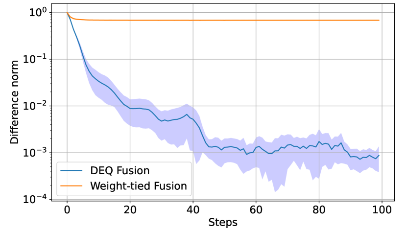
Convergence of DEQ Fusion. We examine the convergence of our DEQ fusion, which is an important assumption since fusion may collapse if it fails to find the equilibrium. We train a model with our DEQ fusion from scratch, and track the relative difference norm evaluated as ${\|\mathbf{z}_{\mathrm{fuse}}^{[i+1]}-\mathbf{z}_{\mathrm{fuse}}^{[i]}\|}/{\|\mathbf{z}_{\mathrm{fuse}}^{[i]}\|}$ over 100 solver steps during inference. We compare it with a weight-tied fusion approach which simply iterates our fusion layer and performs backward pass layer-by-layer. Fig. 3 depicts the empirical results. It is notable that the difference norm of our DEQ fusion quickly drops below 0.01 on average within 20 solver steps, whereas the weight-tied fusion oscillates around a relatively high value. Benefiting from fixed point solvers and analytical backward pass, our DEQ fusion has much quicker and stabler convergence to the fixed point than the weight-tied approach.

References

- [1] Brandon Amos and J Zico Kolter. Optnet: Differentiable optimization as a layer in neural networks. In International Conference on Machine Learning, pages 136–145. PMLR, 2017.
- [2] Donald G Anderson. Iterative procedures for nonlinear integral equations. Journal of the ACM (JACM), 12(4):547–560, 1965.
- [3] John Arevalo, Thamar Solorio, Manuel Montes-y Gómez, and Fabio A González. Gated multimodal units for information fusion. arXiv preprint arXiv:1702.01992, 2017.
- [4] Pradeep K Atrey, M Anwar Hossain, Abdulmotaleb El Saddik, and Mohan S Kankanhalli. Multimodal fusion for multimedia analysis: a survey. Multimedia Systems, 16(6):345–379, 2010.
- [5] Shaojie Bai, Zhengyang Geng, Yash Savani, and J Zico Kolter. Deep equilibrium optical flow estimation. In Proceedings of the IEEE/CVF Conference on Computer Vision and Pattern Recognition, pages 620–630, 2022.
- [6] Shaojie Bai, J Zico Kolter, and Vladlen Koltun. Deep equilibrium models. Advances in Neural Information Processing Systems, 32, 2019.
- [7] Shaojie Bai, Vladlen Koltun, and J Zico Kolter. Multiscale deep equilibrium models. Advances in Neural Information Processing Systems, 33:5238–5250, 2020.
- [8] Shaojie Bai, Vladlen Koltun, and J Zico Kolter. Stabilizing equilibrium models by jacobian regularization. arXiv preprint arXiv:2106.14342, 2021.
- [9] Oresti Banos, Claudia Villalonga, Rafael Garcia, Alejandro Saez, Miguel Damas, Juan A Holgado-Terriza, Sungyong Lee, Hector Pomares, and Ignacio Rojas. Design, implementation and validation of a novel open framework for agile development of mobile health applications. Biomedical Engineering Online, 14(2):1–20, 2015.
- [10] Hedi Ben-Younes, Rémi Cadene, Matthieu Cord, and Nicolas Thome. Mutan: Multimodal tucker fusion for visual question answering. In Proceedings of the IEEE International Conference on Computer Vision, pages 2612–2620, 2017.
- [11] Ricky TQ Chen, Yulia Rubanova, Jesse Bettencourt, and David K Duvenaud. Neural ordinary differential equations. Advances in Neural Information Processing Systems, 31, 2018.
- [12] Jacob Devlin, Ming-Wei Chang, Kenton Lee, and Kristina Toutanova. Bert: Pre-training of deep bidirectional transformers for language understanding. arXiv preprint arXiv:1810.04805, 2018.
- [13] Jiali Duan, Liqun Chen, Son Tran, Jinyu Yang, Yi Xu, Belinda Zeng, and Trishul Chilimbi. Multi-modal alignment using representation codebook. In Proceedings of the IEEE/CVF Conference on Computer Vision and Pattern Recognition, pages 15651–15660, 2022.
- [14] Itai Gat, Idan Schwartz, Alexander Schwing, and Tamir Hazan. Removing bias in multi-modal classifiers: Regularization by maximizing functional entropies. Advances in Neural Information Processing Systems, 33:3197–3208, 2020.
- [15] Yash Goyal, Tejas Khot, Douglas Summers-Stay, Dhruv Batra, and Devi Parikh. Making the v in vqa matter: Elevating the role of image understanding in visual question answering. In Proceedings of the IEEE Conference on Computer Vision and Pattern Recognition, pages 6904–6913, 2017.
- [16] Zongbo Han, Fan Yang, Junzhou Huang, Changqing Zhang, and Jianhua Yao. Multimodal dynamics: Dynamical fusion for trustworthy multimodal classification. In Proceedings of the IEEE/CVF Conference on Computer Vision and Pattern Recognition, pages 20707–20717, 2022.
- [17] Zongbo Han, Changqing Zhang, Huazhu Fu, and Joey Tianyi Zhou. Trusted multi-view classification. arXiv preprint arXiv:2102.02051, 2021.
- [18] Kaiming He, Xiangyu Zhang, Shaoqing Ren, and Jian Sun. Deep residual learning for image recognition. In Proceedings of the IEEE Conference on Computer Vision and Pattern Recognition, pages 770–778, 2016.
- [19] Danfeng Hong, Lianru Gao, Naoto Yokoya, Jing Yao, Jocelyn Chanussot, Qian Du, and Bing Zhang. More diverse means better: Multimodal deep learning meets remote-sensing imagery classification. IEEE Transactions on Geoscience and Remote Sensing, 59(5):4340–4354, 2020.
- [20] Chiori Hori, Takaaki Hori, Teng-Yok Lee, Ziming Zhang, Bret Harsham, John R Hershey, Tim K Marks, and Kazuhiko Sumi. Attention-based multimodal fusion for video description. In Proceedings of the IEEE International Conference on Computer Vision, pages 4193–4202, 2017.
- [21] Ming Hou, Jiajia Tang, Jianhai Zhang, Wanzeng Kong, and Qibin Zhao. Deep multimodal multilinear fusion with high-order polynomial pooling. Advances in Neural Information Processing Systems, 32, 2019.
- [22] Sergey Ioffe and Christian Szegedy. Batch normalization: Accelerating deep network training by reducing internal covariate shift. In International Conference on Machine Learning, pages 448–456. PMLR, 2015.
- [23] Siddhant M. Jayakumar, Jacob Menick, Wojciech M. Czarnecki, Jonathan Schwarz, Jack W. Rae, Simon Osindero, Yee Whye Teh, Tim Harley, and Razvan Pascanu. Multiplicative interactions and where to find them. In International Conference on Learning Representations, 2020.
- [24] Andrej Karpathy, George Toderici, Sanketh Shetty, Thomas Leung, Rahul Sukthankar, and Li Fei-Fei. Large-scale video classification with convolutional neural networks. In Proceedings of the IEEE Conference on Computer Vision and Pattern Recognition, pages 1725–1732, 2014.
- [25] Ryan Kiros, Yukun Zhu, Russ R Salakhutdinov, Richard Zemel, Raquel Urtasun, Antonio Torralba, and Sanja Fidler. Skip-thought vectors. Advances in Neural Information Processing Systems, 28, 2015.
- [26] Guohao Li, Matthias Müller, Bernard Ghanem, and Vladlen Koltun. Training graph neural networks with 1000 layers. In International Conference on Machine Learning, pages 6437–6449. PMLR, 2021.
- [27] Paul Pu Liang, Ziyin Liu, Amir Zadeh, and Louis-Philippe Morency. Multimodal language analysis with recurrent multistage fusion. arXiv preprint arXiv:1808.03920, 2018.
- [28] Paul Pu Liang, Yiwei Lyu, Xiang Fan, Zetian Wu, Yun Cheng, Jason Wu, Leslie Chen, Peter Wu, Michelle A Lee, Yuke Zhu, et al. Multibench: Multiscale benchmarks for multimodal representation learning. arXiv preprint arXiv:2107.07502, 2021.
- [29] Yuanzhi Liang, Yalong Bai, Wei Zhang, Xueming Qian, Li Zhu, and Tao Mei. Vrr-vg: Refocusing visually-relevant relationships. In Proceedings of the IEEE/CVF International Conference on Computer Vision, pages 10403–10412, 2019.
- [30] Yunze Liu, Qingnan Fan, Shanghang Zhang, Hao Dong, Thomas Funkhouser, and Li Yi. Contrastive multimodal fusion with tupleinfonce. In Proceedings of the IEEE/CVF International Conference on Computer Vision, pages 754–763, 2021.
- [31] Ze Liu, Yutong Lin, Yue Cao, Han Hu, Yixuan Wei, Zheng Zhang, Stephen Lin, and Baining Guo. Swin transformer: Hierarchical vision transformer using shifted windows. In Proceedings of the IEEE/CVF International Conference on Computer Vision, pages 10012–10022, 2021.
- [32] Ze Liu, Zheng Zhang, Yue Cao, Han Hu, and Xin Tong. Group-free 3d object detection via transformers. In Proceedings of the IEEE/CVF International Conference on Computer Vision, pages 2949–2958, 2021.
- [33] Zhun Liu, Ying Shen, Varun Bharadhwaj Lakshminarasimhan, Paul Pu Liang, Amir Zadeh, and Louis-Philippe Morency. Efficient low-rank multimodal fusion with modality-specific factors. arXiv preprint arXiv:1806.00064, 2018.
- [34] Cheng Lu, Jianfei Chen, Chongxuan Li, Qiuhao Wang, and Jun Zhu. Implicit normalizing flows. arXiv preprint arXiv:2103.09527, 2021.
- [35] Youssef Mroueh, Etienne Marcheret, and Vaibhava Goel. Deep multimodal learning for audio-visual speech recognition. In 2015 IEEE International Conference on Acoustics, Speech and Signal Processing (ICASSP), pages 2130–2134. IEEE, 2015.
- [36] Arsha Nagrani, Shan Yang, Anurag Arnab, Aren Jansen, Cordelia Schmid, and Chen Sun. Attention bottlenecks for multimodal fusion. Advances in Neural Information Processing Systems, 34:14200–14213, 2021.
- [37] Pradeep Natarajan, Shuang Wu, Shiv Vitaladevuni, Xiaodan Zhuang, Stavros Tsakalidis, Unsang Park, Rohit Prasad, and Premkumar Natarajan. Multimodal feature fusion for robust event detection in web videos. In 2012 IEEE Conference on Computer Vision and Pattern Recognition, pages 1298–1305. IEEE, 2012.
- [38] Ara V. Nefian, Luhong Liang, Xiaobo Pi, Xiaoxing Liu, and Kevin P. Murphy. Dynamic bayesian networks for audio-visual speech recognition. EURASIP Journal on Advances in Signal Processing, 2002:1–15, 2002.
- [39] Jiquan Ngiam, Aditya Khosla, Mingyu Kim, Juhan Nam, Honglak Lee, and Andrew Y Ng. Multimodal deep learning. In International Conference on Machine Learning, 2011.
- [40] Juan DS Ortega, Mohammed Senoussaoui, Eric Granger, Marco Pedersoli, Patrick Cardinal, and Alessandro L Koerich. Multimodal fusion with deep neural networks for audio-video emotion recognition. arXiv preprint arXiv:1907.03196, 2019.
- [41] Yingwei Pan, Ting Yao, Yehao Li, and Tao Mei. X-linear attention networks for image captioning. In Proceedings of the IEEE/CVF Conference on Computer Vision and Pattern Recognition, pages 10971–10980, 2020.
- [42] Jeffrey Pennington, Richard Socher, and Christopher D Manning. Glove: Global vectors for word representation. In Proceedings of the 2014 Conference on Empirical Methods in Natural Language Processing (EMNLP), pages 1532–1543, 2014.
- [43] Juan-Manuel Pérez-Rúa, Valentin Vielzeuf, Stéphane Pateux, Moez Baccouche, and Frédéric Jurie. Mfas: Multimodal fusion architecture search. In Proceedings of the IEEE/CVF Conference on Computer Vision and Pattern Recognition, pages 6966–6975, 2019.
- [44] Hai Pham, Paul Pu Liang, Thomas Manzini, Louis-Philippe Morency, and Barnabás Póczos. Found in translation: Learning robust joint representations by cyclic translations between modalities. In Proceedings of the AAAI Conference on Artificial Intelligence, volume 33, pages 6892–6899, 2019.
- [45] Fernando Pineda. Generalization of back propagation to recurrent and higher order neural networks. In Neural Information Processing Systems, 1987.
- [46] Ashwini Pokle, Zhengyang Geng, and Zico Kolter. Deep equilibrium approaches to diffusion models. arXiv preprint arXiv:2210.12867, 2022.
- [47] Charles R Qi, Xinlei Chen, Or Litany, and Leonidas J Guibas. Imvotenet: Boosting 3d object detection in point clouds with image votes. In Proceedings of the IEEE/CVF Conference on Computer Vision and Pattern Recognition, pages 4404–4413, 2020.
- [48] Charles R Qi, Or Litany, Kaiming He, and Leonidas J Guibas. Deep hough voting for 3d object detection in point clouds. In Proceedings of the IEEE/CVF International Conference on Computer Vision, pages 9277–9286, 2019.
- [49] Dhanesh Ramachandram and Graham W Taylor. Deep multimodal learning: A survey on recent advances and trends. IEEE Signal Processing Magazine, 34(6):96–108, 2017.
- [50] Sethuraman Sankaran, David Yang, and Ser-Nam Lim. Multimodal fusion refiner networks. arXiv preprint arXiv:2104.03435, 2021.
- [51] Karen Simonyan and Andrew Zisserman. Two-stream convolutional networks for action recognition in videos. Advances in Neural Information Processing Systems, 27, 2014.
- [52] Shuran Song, Samuel P Lichtenberg, and Jianxiong Xiao. Sun rgb-d: A rgb-d scene understanding benchmark suite. In Proceedings of the IEEE Conference on Computer Vision and Pattern Recognition, pages 567–576, 2015.
- [53] Zhongkai Sun, Prathusha Sarma, William Sethares, and Yingyu Liang. Learning relationships between text, audio, and video via deep canonical correlation for multimodal language analysis. In Proceedings of the AAAI Conference on Artificial Intelligence, volume 34, pages 8992–8999, 2020.
- [54] Zachary Teed and Jia Deng. Raft: Recurrent all-pairs field transforms for optical flow. In European Conference on Computer Vision, pages 402–419. Springer, 2020.
- [55] Yao-Hung Hubert Tsai, Shaojie Bai, Paul Pu Liang, J Zico Kolter, Louis-Philippe Morency, and Ruslan Salakhutdinov. Multimodal transformer for unaligned multimodal language sequences. In Proceedings of the conference. Association for Computational Linguistics. Meeting, volume 2019, page 6558. NIH Public Access, 2019.
- [56] Yao-Hung Hubert Tsai, Paul Pu Liang, Amir Zadeh, Louis-Philippe Morency, and Ruslan Salakhutdinov. Learning factorized multimodal representations. arXiv preprint arXiv:1806.06176, 2018.
- [57] Mark A Van De Wiel, Tonje G Lien, Wina Verlaat, Wessel N van Wieringen, and Saskia M Wilting. Better prediction by use of co-data: adaptive group-regularized ridge regression. Statistics in Medicine, 35(3):368–381, 2016.
- [58] Ashish Vaswani, Noam Shazeer, Niki Parmar, Jakob Uszkoreit, Llion Jones, Aidan N Gomez, Łukasz Kaiser, and Illia Polosukhin. Attention is all you need. Advances in Neural Information Processing Systems, 30, 2017.
- [59] Valentin Vielzeuf, Alexis Lechervy, Stéphane Pateux, and Frédéric Jurie. Centralnet: a multilayer approach for multimodal fusion. In Proceedings of the European Conference on Computer Vision (ECCV) Workshops, pages 0–0, 2018.
- [60] Tongxin Wang, Wei Shao, Zhi Huang, Haixu Tang, Jie Zhang, Zhengming Ding, and Kun Huang. Mogonet integrates multi-omics data using graph convolutional networks allowing patient classification and biomarker identification. Nature Communications, 12(1):1–13, 2021.
- [61] Yikai Wang, Wenbing Huang, Fuchun Sun, Tingyang Xu, Yu Rong, and Junzhou Huang. Deep multimodal fusion by channel exchanging. Advances in Neural Information Processing Systems, 33:4835–4845, 2020.
- [62] Yuxin Wu and Kaiming He. Group normalization. In Proceedings of the European Conference on Computer Vision (ECCV), pages 3–19, 2018.
- [63] Huijuan Xu, Kun He, Leonid Sigal, Stan Sclaroff, and Kate Saenko. Text-to-clip video retrieval with early fusion and re-captioning. arXiv preprint arXiv:1804.05113, 2018.
- [64] Zihui Xue and Radu Marculescu. Dynamic multimodal fusion. arXiv preprint arXiv:2204.00102, 2022.
- [65] Kaicheng Yang, Hua Xu, and Kai Gao. Cm-bert: Cross-modal bert for text-audio sentiment analysis. In Proceedings of the 28th ACM International Conference on Multimedia, pages 521–528, 2020.
- [66] Guangnan Ye, Dong Liu, I-Hong Jhuo, and Shih-Fu Chang. Robust late fusion with rank minimization. In 2012 IEEE Conference on Computer Vision and Pattern Recognition, pages 3021–3028. IEEE, 2012.
- [67] Zhou Yu, Jun Yu, Yuhao Cui, Dacheng Tao, and Qi Tian. Deep modular co-attention networks for visual question answering. In Proceedings of the IEEE/CVF Conference on Computer Vision and Pattern Recognition, pages 6281–6290, 2019.
- [68] Amir Zadeh, Paul Pu Liang, Navonil Mazumder, Soujanya Poria, Erik Cambria, and Louis-Philippe Morency. Memory fusion network for multi-view sequential learning. In Proceedings of the AAAI Conference on Artificial Intelligence, volume 32, 2018.
- [69] Amir Zadeh, Paul Pu Liang, Soujanya Poria, Prateek Vij, Erik Cambria, and Louis-Philippe Morency. Multi-attention recurrent network for human communication comprehension. In Proceedings of the AAAI Conference on Artificial Intelligence, volume 32, 2018.
- [70] Amir Zadeh, Rowan Zellers, Eli Pincus, and Louis-Philippe Morency. Mosi: multimodal corpus of sentiment intensity and subjectivity analysis in online opinion videos. arXiv preprint arXiv:1606.06259, 2016.
Appendix A Proof for Backpropagation of DEQ Fusion
Proof of Theorem 1.
Our proof is similar to [6]. We know from Eq. 14, we can first differentiate two sides implicitly with respect to :