DeDrift: Robust Similarity Search under Content Drift
Abstract
The statistical distribution of content uploaded and searched on media sharing sites changes over time due to seasonal, sociological and technical factors. We investigate the impact of this “content drift” for large-scale similarity search tools, based on nearest neighbor search in embedding space. Unless a costly index reconstruction is performed frequently, content drift degrades the search accuracy and efficiency. The degradation is especially severe since, in general, both the query and database distributions change.
We introduce and analyze real-world image and video datasets for which temporal information is available over a long time period. Based on the learnings, we devise DeDrift, a method that updates embedding quantizers to continuously adapt large-scale indexing structures on-the-fly. DeDrift almost eliminates the accuracy degradation due to the query and database content drift while being up to faster than a full index reconstruction.
1 Introduction

The amount of content available online is growing exponentially over the years. Various online content sharing sites collect billions to trillions of images, videos and posts over time. Efficient Nearest Neighbor Search (NNS) techniques enable searching these vast unstructured databases based on content similarity. NNS is at the core of a plethora of practical machine learning applications including content moderation [17], retrieval augmented modeling [10, 24], keypoint matching for 3D reconstruction [1], image-based geo-localisation [12], content de-duplication [44], k-NN classification [4, 11], defending against adversarial attacks [18], active learning [15] and many others.
NNS techniques extract high dimensional feature vectors (a.k.a. “embeddings”) from each item to be indexed. These embeddings may be computed by hand-crafted techniques [35, 28] or, more commonly nowadays, with pre-trained neural networks [7, 37, 36]. Given the database of embedding vectors and a query embedding , NNS retrieves the closest database example to from according to some similarity measure, typically the L2 distance:
| (1) |
The exact nearest neighbor and its distance can be computed by exhaustively comparing the query embeddings against the entire database. On a single core of a typical server from 2023, this brute-force solution takes a few milliseconds for databases smaller than few tens of thousand examples with embeddings up to a few hundred dimensions.
However, practical use cases require real time search on millions to trillion size databases, where brute-force NNS is too slow [14]. Practitioners resort to approximate NNS (ANNS), trading some accuracy of the results to speed up the search. A common approach is to perform a statistical analysis of to build a specialized data structure (an “index” in database terms) that performs the search efficiently. Like any unsupervised machine learning task, the index is trained on representative sample vectors from the data distribution to the index.
A tool commonly used in indexes is vector quantization [22]. It consists in representing each vector by the nearest vector taken in a finite set of centroids . A basic use of quantization is compact storage: the vector can be reduced to the index of the centroid it is assigned to, which occupies just bits of storage. The larger , the better the approximation. As typical for machine learning, the training set is distinct from (usually is a small subset of ). The unsupervised training algorithm of choice for quantization is k-means which guarantees Lloyd’s optimality conditions [32].
In an online media sharing site, the index functions as a database system. After the initial training, the index ingests new embeddings by batches as they are uploaded by users and removes content that has been deleted (Figure 1). Depending on the particular indexing structure, addition/deletion may be easy [27], or more difficult [40]. However, a more pernicious problem that appears over the time is content drift. In practice, over months and years, the statistical distribution of the content changes slowly, both for the data inserted in the index and the items that are queried.
The drift on image content may have a technical origin, e.g. camera images become sharper and have better contrast; post-processing tools evolve as many platforms offer editing options with image filters that are applied to millions of images. The drift may be seasonal: the type of photos that are taken in summer is not the same as in winter, see Figure 2. Sociological causes could be that people post pictures of leaderboards of a game that became viral, or there is a lockdown period where people share only indoor pictures without big crowds. In rare cases, the distribution may also change suddenly, for example because of an update of the platform that changes how missing images are displayed. The problem posed by this distribution drift is that new incoming vectors are distributed differently from . Indeed, by design, feature extractors are sensitive to semantic differences in the content. This mismatch between training and indexed vectors impacts the search accuracy negatively. To address this, practitioners monitor the indexing performance and initiate a full index reconstruction once the efficiency degrades noticeably. By definition, this is the optimal update strategy since it adapts exactly to the new data distribution that contains both old and recent vectors. However, at larger scales, this operation becomes a resource bottleneck since all vectors need to be re-added to the index, and disrupts the services that relies on the index.
Our first contribution is to carefully investigate temporal distribution drift in the context of large-scale nearest neighbor search. For this purpose, we introduce two real-world datasets that exhibit drift. We first measure the drift in an index-agnostic way, on exact search queries (Section 3). Then we measure the impact on various index types that are commonly used for large-scale vector search (Section 4).
Our second contribution is DeDrift, a family of adaptation strategies applied to the most vulnerable index types (Section 5). DeDrift modifies the index slightly to adapt to the evolution of the vector distribution, without re-indexing all the stored elements, which would incur an cost. This adaptation yields search results that are close to the reindexing topline while being orders of magnitude faster. This modification is done while carefully controlling the accuracy degradation. Sections 6 reports and analyzes DeDrift’s results.
2 Related work
NNS methods. In low-dimensional spaces, NNS can be solved efficiently and exactly with tree structures like the KD-tree [19, 33] and ball-trees [34], that aim at achieving a search time logarithmic in . However, in higher dimensions, due to the curse of dimensionality, the tree structures are ineffective to prune the search space, so there is no efficient exact solution. Therefore, practitioners use approximate NNS (ANNS) methods, trading some accuracy to improve the efficiency. Early ANNS methods rely on data-independent structures, e.g. projections on fixed random directions [2, 16]. However, the most efficient methods adapt to the data distribution using vector quantization.
The Inverted File (IVF) based indexing relies on a vector quantizer (the coarse quantizer) to partition the database vectors into clusters [41, 27]. At search time, only one or a few of these clusters need to be checked for result vectors. Such pruning approach is required to search in large datasets, so we focus on IVF-based methods in this paper. When scaling up the coarse quantizer can become the computation bottleneck. Several alternatives to plain k-means have been proposed: the inverted multi-index uses a product quantizer [6], graph-based indexes [8] or residual quantizers can also be used [13].
Out-of-distribution (OOD) vectors w.r.t the training distribution are detrimental to the search performance [39]. For IVF based methods, they translate to unbalanced cluster sizes, which incurs a slowdown that can be quantified by an imbalance factor [26]. In [47], OOD content is addressed before indexing with LSH by adapting a transformation matrix, but LSH’s accuracy is limited by its low adaptability to the data distribution. Graph-based pruning methods like HNSW [46] also suffer from OOD queries [25]. In this work, our focus is not on graph-based indexes since they do not scale as well to large datasets.
Database drift. In the literature, ANNS studies are primarily on publicly available offline vector databases where the distribution of query and database examples are fixed and often sampled from the same underlying data distribution [29, 5]. However, these assumptions do not typically hold for real world applications. Not only the query frequency and database size, but also their distributions may drift over time. Recent works [45, 31] simulate this setting and propose adaptive vector encoding methods. In our work, we collect the data with natural content drift and observe that vector codecs are relatively robust to content changes, as opposed to IVF-based indexing structures. Another work [9] adapts the k-means algorithm to take the drift into account. Though this method can improve the performance of IVF indexes, it still requires full index reconstruction.
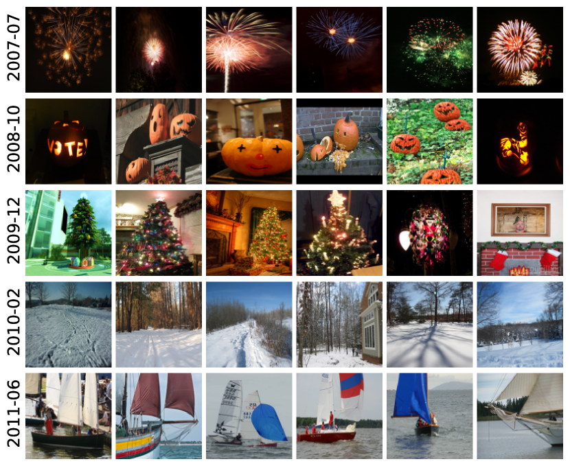
Image credits: see Appendix J |
| VideoAds | |
 |
 |
| YFCC | |
 |
 |
3 Temporal statistics of user generated content
We present the two representative datasets and report some statistics about them.
3.1 Datasets
We introduce two real-world datasets to serve as a basis for the drift analysis. In principle, most content collected over several years exhibits some form of drift. For the dataset collection, the constraints are (1) the content should be collected over a long time period (2) the volume should be large enough that statistical trends become apparent (3) the data source should be homogeneous so that other sources of noise are minimized (4) of course, timestamps should be available, either for the data acquisition or the moment the data is uploaded.
The VideoAds dataset contains “semantic”111We call “semantic” embeddings that are intended for input to classifiers. In contrast, copy detection embeddings identify lower-level features useful for image matching [36]. embeddings extracted from ads videos published on a large social media website between October and October . The ads are of professional and non-professional quality, published by individuals, small and large businesses. They were clipped to be of maximum seconds in length. The video encoder for the video ads consisted of a RegNetY [38] frame encoder followed by a Linformer [43] temporal pooling layer which were trained using MoCo [23], resulting in one embedding per video. The dataset contains L2-normalized embeddings in dimensions.
The YFCC dataset [42] contains 100M images and videos from the Yahoo Flickr photo sharing site. Compared to typical user-generated content sites, Flickr images are of relatively good quality because uploads are limited and users are mostly pro or semi-pro photographers. We filter out videos, broken dates and dummy images of uniform color, leaving usable images spanning years, from January 2007 to December 2013. As a feature extractor, we use a pretrained DINO [11] model with ViT-S/16 backbone that outputs unnormalized 384-dimensional vectors. As DINO embeddings have been developed for use as k-NN classifiers, their L2 distances are semantically meaningful.
Before evaluations, we apply a random rotation to all embeddings and uniformly quantize them to bits to make them less bulky. These operations have almost no impact on neighborhood relations. We do not apply dimensionality reduction methods, e.g., PCA, since it can be considered as a part of the indexing method and explored separately.
3.2 Volume of data
First, we depict daily and monthly traffic for both datasets in Figure 3. For VideoAds, the traffic is lower during weekends and slightly increases over years. For YFCC, the traffic is higher on weekends than on weekdays. This pattern is due to the professional vs. personal nature of the data.
Over the years, the amount of content also grows for both datasets, following the organic growth of online traffic. Interestingly, for YFCC, we observe minimum traffic in January and maximum in July. In the following, we use subsampling to cancel the statistical effect of data volume. Unless stated, we use a monthly granularity because this is the typical scale at which drift occurs.
| VideoAds | YFCC |
| Oct 2020 Sep 2022 | Jan 2007 Dec 2013 |

|

|
3.3 Per-month similarities
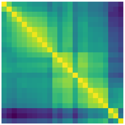
We start the analysis of temporal distribution drift by visualizing pairwise similarities between months and . For each month, we sample a random set of embeddings. Then, we compute the similarity between and by averaging nearest-neighbor distances:
| (2) | |||
| (3) |
where and is the -th nearest neighbor of in . Note that the similarity is asymmetric: in general. Figure 4 shows the similarity matrices for VideoAds and YFCC datasets. The analysis with daily and weekly granularities is in Appendix A.
We observe that the ads data changes over time but does not have noticeable patterns. YFCC content drifts over years and has a strong seasonal dependency. Figure 2 presents images from YFCC for different seasons222 The images for the month were selected as follows: a quantizer of size is trained on . Vectors from and are assigned to the centroids independently. We visualize six random images from one of the top-8 clusters where the size ratio between assignment over assignment is the largest. Out of these 8, we select one representative cluster for visualization. the seasonal pattern is caused by images of outdoor sceneries (e.g., snow and foliage), seasonal activities (e.g., yachting) or holidays (e.g., Halloween and Christmas). Appendix B studies the impact of these monthly similarity patterns on the distribution of quantization assignments.
| VideoAds | YFCC |

3.4 Temporal distribution of nearest neighbors
In this experiment, we investigate the distribution of the nearest neighbors results over predefined time periods. We consider queries for month and search exact top-k (k) results in ( for VideoAds and for YFCC). Figure 5 shows how many of the nearest neighbors come from each of the previous months for a few settings of the reference month . We observe that recent content occurs more often in the results for both datasets. Also, for YFCC, there is a clear seasonal trend, i.e. content from the same season in years before is more likely to be returned. This hints at a drift because if the vectors were temporally i.i.d. search results would be equally likely to come from all previous months.
4 Content drift with static indexes
In this section, we assess the effect of content drift for various index types.
4.1 Experimental setting
The evaluation protocol follows a common use case, where the most recent content is used as query data against a backlog of older content.
Data streaming. The index is trained on months and months are added to the index, where is a window size. In the in-domain (ID) setting, the training is performed on the same data as the indexed vectors (). In the out-of-domain (OOD) setting, the training and indexing time ranges are different (, the first month of the time series and ). If not stated otherwise, we consider months as it is the maximum retention period of user data for many sharing platforms.
Over time, the index content is updated using a sliding window with a time step 1 month: at each month, we remove the data for the oldest month and insert the data for the next month. The queries are a random subset of 10,000 vectors for the month . This setting mimics the real-world setting when queries come after the index is constructed.
Metrics. Our ground truth is simply the exact k-NN results from brute force search. As a primary quality measure, we use , the fraction of ground-truth -nearest neighbors found in the top results retrieved by the search algorithm () [39]. For IVF-based indexes, the efficiency measure is the number of distance calculations (DCS) between the query vector and database entries [6]. At search time, the DCS is given as a fixed “budget”: for a query vector , clusters are visited staring from the nearest centroid to . The distances between and all vectors in the clusters are computed until the DCS budget is exhausted (only a fraction of the vectors of the last cluster may be processed). The advantage of this measure over direct timings is that it is independent of the hardware. Appendix G reports search time equivalents for a few settings.
Evaluation. We evaluate the k-recall@k after each content update step over the entire time range. For each index type and DCS setting, we focus on the month where the gap between the ID and OOD settings is the largest.
4.2 Robustness of static indexing methods
In this section, we investigate the robustness of static indexes of the IVF family. Graph-based indexes [46, 20] are not in the scope of this study because they don’t scale as well to billion-scale datasets. The components of an IVF index are (1) the codec that determines how the vectors are encoded for in-memory storage (2) the coarse quantizer that determines how the database vectors are clustered.
Vector codecs decrease the size of the vectors for in-memory storage. We consider PCA dimensionality reduction to and dimensions and quantization methods PQ and OPQ [27, 21] to reduce vectors to and bytes. To make results independent of the IVF structure, we measure the 10-recall@10 with an exhaustive comparison between the queries and all vectors in . In Table 1, we observe a small gap for most settings (). We attribute this to the small codebook sizes of the codecs. In ML terms, they can hardly fit the data and, hence, may be less sensitive to the drift.
| VideoAds | YFCC | |||
|---|---|---|---|---|
| Method | ID | OOD | ID | OOD |
| 0.709 | \cellcolor[HTML]d7ffb2 0.698 | 0.625 | \cellcolor[HTML]bcffb2 0.622 | |
| 0.844 | \cellcolor[HTML]d1ffb2 0.835 | 0.867 | \cellcolor[HTML]bcffb2 0.864 | |
| 0.237 | \cellcolor[HTML]b2ffb2 0.237 | 0.164 | \cellcolor[HTML]bfffb2 0.160 | |
| 0.441 | \cellcolor[HTML]b2ffb2 0.441 | 0.380 | \cellcolor[HTML]bcffb2 0.377 | |
| 0.457 | \cellcolor[HTML]d7ffb2 0.446 | 0.302 | \cellcolor[HTML]ccffb2 0.294 | |
| 0.609 | \cellcolor[HTML]ccffb2 0.601 | 0.484 | \cellcolor[HTML]c9ffb2 0.477 | |
| Budget | 6000 DCS | 12000 DCS | 30000 DCS | 60000 DCS | ||||
|---|---|---|---|---|---|---|---|---|
| Method | ID | OOD | ID | OOD | ID | OOD | ID | OOD |
| IVF | 0.842 | \cellcolor[HTML]ffb2be 0.732 | 0.914 | \cellcolor[HTML]ffb2be 0.845 | 0.966 | \cellcolor[HTML]ffefb2 0.938 | 0.985 | \cellcolor[HTML]dbffb2 0.973 |
| IVF | 0.914 | \cellcolor[HTML]ffb2be 0.835 | 0.956 | \cellcolor[HTML]ffb3b2 0.910 | 0.984 | \cellcolor[HTML]ebffb2 0.967 | 0.993 | \cellcolor[HTML]ccffb2 0.985 |
| IMI | 0.257 | \cellcolor[HTML]dbffb2 0.245 | 0.391 | \cellcolor[HTML]fff2b2 0.364 | 0.662 | \cellcolor[HTML]ffb2be 0.592 | 0.838 | \cellcolor[HTML]ffb2be 0.775 |
| IMI | 0.529 | \cellcolor[HTML]ffb2be 0.469 | 0.732 | \cellcolor[HTML]ffb2be 0.651 | 0.891 | \cellcolor[HTML]ffb2be 0.841 | 0.951 | \cellcolor[HTML]feffb2 0.928 |
| RCQ | 0.651 | \cellcolor[HTML]ffb2be 0.531 | 0.776 | \cellcolor[HTML]ffb2be 0.676 | 0.899 | \cellcolor[HTML]ffb2be 0.838 | 0.951 | \cellcolor[HTML]ffd6b2 0.916 |
| RCQ | 0.809 | \cellcolor[HTML]ffb2be 0.713 | 0.895 | \cellcolor[HTML]ffb2be 0.826 | 0.958 | \cellcolor[HTML]ffddb2 0.925 | 0.981 | \cellcolor[HTML]e4ffb2 0.966 |
| Budget | 6000 DCS | 12000 DCS | 30000 DCS | 60000 DCS | ||||
| Method | ID | OOD | ID | OOD | ID | OOD | ID | OOD |
| IVF | 0.796 | \cellcolor[HTML]ffb2be 0.744 | 0.892 | \cellcolor[HTML]ffd9b2 0.858 | 0.960 | \cellcolor[HTML]e4ffb2 0.945 | 0.983 | \cellcolor[HTML]c5ffb2 0.977 |
| IVF | 0.894 | \cellcolor[HTML]ffbcb2 0.851 | 0.947 | \cellcolor[HTML]fff8b2 0.922 | 0.981 | \cellcolor[HTML]d1ffb2 0.972 | 0.993 | \cellcolor[HTML]bfffb2 0.989 |
| IMI | 0.245 | \cellcolor[HTML]ffefb2 0.217 | 0.409 | \cellcolor[HTML]ffb2bb 0.360 | 0.727 | \cellcolor[HTML]ffb3b2 0.681 | 0.872 | \cellcolor[HTML]bcffb2 0.869 |
| IMI | 0.449 | \cellcolor[HTML]ffe6b2 0.419 | 0.673 | \cellcolor[HTML]ffb3b2 0.627 | 0.870 | \cellcolor[HTML]feffb2 0.847 | 0.948 | \cellcolor[HTML]d4ffb2 0.938 |
| RCQ | 0.575 | \cellcolor[HTML]ffb2be 0.521 | 0.730 | \cellcolor[HTML]ffb2b8 0.682 | 0.878 | \cellcolor[HTML]ffefb2 0.850 | 0.940 | \cellcolor[HTML]deffb2 0.927 |
| RCQ | 0.768 | \cellcolor[HTML]ffb2be 0.718 | 0.872 | \cellcolor[HTML]ffddb2 0.839 | 0.949 | \cellcolor[HTML]e8ffb2 0.933 | 0.978 | \cellcolor[HTML]c9ffb2 0.971 |
The coarse quantizer partitions the search space. We evaluate the following coarse quantizers with centroids: IVF is the plain k-means [27]; IMI a product quantizer with two sub-vectors [6] each quantized to centroids (); and RCQ_ is a two-level residual quantizer [13], where the quantizers are of sizes and centroids ().
Table 2 reports the 10-recall@10 for various DCS budgets representing different operating points. We experiment with different index settings for VideoAds and YFCC, due to their size difference. The content drift has a significant impact in these experiments. We investigate the effect of different window sizes in Appendix C.
5 Updating the index to accomodate data drift
In this section, we introduce DeDrift to reduce the impact of data drift on IVF indexes over time. First, we address the case where vectors are partitioned by the IVF but stored exactly. Then we show how to handle compressed vectors.
Our baseline methods are the lower and upper bounds of the accuracy: None keeps the trained part of the quantizer untouched over the entire time span; with Full, the index is reconstructed at each update step.
5.1 DeDrift updating strategies
DeDrift-Split addresses imbalance by repartitioning a few clusters. DeDrift-Split collects the vectors from the largest clusters into . The objective is to re-assign these vectors into new clusters, where is chosen so that the average new cluster size is the median cluster size of the whole IVF: . To keep the total number of clusters constant, vectors from the smallest clusters are collected into . We train k-means with centroids on , and replace the involved clusters in the index. Other centroids and clusters are left untouched, so the update cost is much lower than .
DeDrift-Lazy updates all centroids by recomputing the centroid of the vectors assigned to each cluster. In contrast to a full k-means iteration, the vectors are not re-assigned after the centroid update. Therefore, DeDrift-Lazy smoothly adapts the centroids to the shifting distribution without a costly re-assignment operation. The similar idea was previously considered in the context of VLAD descriptors [3].
DeDrift-Hybrid combines Split and Lazy by updating the centroids first, then splitting largest clusters.
Discussion. In a non-temporal setting, if the query and database vectors were sampled uniformly from the whole time range, they would be i.i.d. and the optimal quantizer would be k-means (if it could reach the global optimum). The DeDrift approaches are heuristic, they do not offer k-means’ optimality guarantees. However, our setting is different: (1) the database is incremental, so we want to avoid doing a costly global k-means and (2) the query vectors are the most recent ones, so the i.i.d. assumption is incorrect. Reason (1) means that we have to fall back to heuristics to “correct” the index on-the-fly and (2) means that DeDrift heuristics may actually outperform a full re-indexing.
5.2 DeDrift in the compressed domain
For billion-scale datasets, the vectors stored in the IVF are compressed with codecs, see Section 4.2. However, DeDrift-Split needs to access all original embeddings (e.g. from external storage). Besides, DeDrift-Lazy needs to update centroids using the original vectors. Reconstructed vectors could be used but this significantly degrades the performance of the DeDrift variants (see Appendix H). A workaround for DeDrift-Lazy is to store just a subsampled set of training vectors. There is no such workaround for the other methods: they must store the entire database, which is an operational constraint.
Efficient DeDrift-Lazy with PQ compression.
We focus on the product quantizer (PQ), which is the most prevalent and difficult to update vector codec. There are two ways to store a database vector in an IVF index: compress directly (Section 4.2 shows that drift does not affect this much), or store by residual [27], which is more accurate. When storing by residual, the vector that gets compressed is relative to the centroid that is assigned to: is compressed to an approximation .
The distance between a query and the compressed vector is computed in the compressed domain, without decompressing . For the L2 distance, this relies on distance look-up tables that are built for every pair, i.e. when starting to process a cluster in the index. The look-up tables are of size for a PQ of sub-quantizers of entries. In a static index, one query gets compared to the vectors of clusters ( a.k.a. ), so look-up tables are computed times. The runtime cost of computing look-up tables is FLOPs.
In DeDrift-Lazy, there are successive “versions” of . Computing the look-up tables with only the latest version of incurs an unacceptable accuracy impact, so we need to compute look-up tables for each time step. For this, we (1) store the history of ’s values and (2) partition the vectors within each cluster into subsets, based on the version that they were encoded with.
The additional index storage required for the historical centroids is in the order of floats. For example, for , , , and PQ32 encoding, the historical centroids stored in float16 will consume of the PQ codes. This may be considered significant, especially for large settings. In the future work, we anticipate addressing this limitation of our approach.
The additional computations required for the look-up tables is FLOPs. For large-scale static indexes, the time to build the look-up tables is small compared to the compressed-domain distance computations. This remains true for small values of .
Note that the coarse quantization is still performed on centroids and the residuals w.r.t. historical centroids are computed only for the nearest centroids.
| YFCC June 2013 | VideoAds June 2022 |


6 Experimental results
Here, we evaluate DeDrift empirically. All experiments are performed with the FAISS library [30], with the protocol in Section 4.1: ANNS under a fixed budget of distance computations (DCS). Unless specified, we report the results at one time step chosen to maximize the average recall gap between the None and Full settings over the DCS budgets.
| Budget (DCS) | 6000 | 12000 | 20000 | 30000 | 60000 |
|---|---|---|---|---|---|
| None | \cellcolor[HTML]ffb2be 0.726 | \cellcolor[HTML]ffc9b2 0.865 | \cellcolor[HTML]fff8b2 0.917 | \cellcolor[HTML]deffb2 0.950 | \cellcolor[HTML]ccffb2 0.976 |
| Split | \cellcolor[HTML]ffefb2 0.796 | \cellcolor[HTML]f4ffb2 0.884 | \cellcolor[HTML]e4ffb2 0.927 | \cellcolor[HTML]dbffb2 0.951 | \cellcolor[HTML]c9ffb2 0.977 |
| Lazy | \cellcolor[HTML]ffb2be 0.720 | \cellcolor[HTML]ffb2be 0.796 | \cellcolor[HTML]ffb2be 0.832 | \cellcolor[HTML]ffb2be 0.868 | \cellcolor[HTML]ffcdb2 0.946 |
| Hybrid | \cellcolor[HTML]b2ffb2 0.824 | \cellcolor[HTML]bfffb2 0.900 | \cellcolor[HTML]c2ffb2 0.937 | \cellcolor[HTML]bfffb2 0.959 | \cellcolor[HTML]bfffb2 0.980 |
| Full | \cellcolor[HTML]b2ffb2 0.824 | \cellcolor[HTML]b2ffb2 0.904 | \cellcolor[HTML]b2ffb2 0.942 | \cellcolor[HTML]b2ffb2 0.963 | \cellcolor[HTML]b2ffb2 0.984 |
6.1 Uncompressed embeddings
First, we consider DeDrift on IVF methods with uncompressed embeddings. We consider the quantizer is updated every 1, 2, 3 or 6 months to see how long it can be frozen without perceptible loss in performance.
Along with the recall, we measure the average index update time. The IVF contain centroids for VideoAds and for YFCC (accounting to the different numbers of vectors within months).
Figure 6 shows that DeDrift-Split improves the search performance especially for low DCS budgets, while it is (resp. ) more efficient than the index reconstruction (Full) on YFCC (resp. VideoAds). DeDrift-Lazy significantly outperforms DeDrift-Split on both datasets and all DCS budgets, and is still (YFCC) and (VideoAds) faster than Full. DeDrift-Hybrid further improves the DeDrift-Lazy performance for low DCS.
Overall, DeDrift almost reaches Full on YFCC and significantly reduces the gap between Full and None on VideoAds. e.g., on YFCC, the proposed method provides , and gains for , and DCS budgets, respectively. DeDrift is about two orders of magnitude cheaper than the full index reconstruction.
In Appendix I, we evaluate Full with evolving k-means [9] which adapts the k-means algorithm to the drift. This provides slightly higher recall on both datasets. However, the update costs are similar to the full index reconstruction.
Hyperparameters. We vary crucial parameters for the DeDrift variants. For DeDrift-Split, we consider and clusters for the YFCC and VideoAds datasets, respectively. Higher values usually lead to slightly better recall rates at the cost of noticeably higher index update costs. DeDrift-Lazy performs a single centroid update at a time. Appendix D shows that more training iterations tend to degrade the performance. We hypothesize that further training moves the centroids too far away from the vectors already stored to represent them accurately.
6.2 Robustness to outlier content
We investigate the index robustness to outlier content that occasionally occurs in real-world settings. When starting experiments on the YFCC dataset, we observed bursts of images of uniform color. It turns out these are placeholders for removed images. For the previous experiments, we removed these in the cleanup phase.
To assess DeDrift’s robustness, we add these images back to the YFCC dataset and repeat the experiments from Section 6.1. Table 3 shows results for September 2012 (month with the largest None-Full gap): DeDrift-Lazy significantly degrades compared to all methods, including no reindexing (None). In contrast, DeDrift-Split and DeDrift-Hybrid prevent the performance drop, Hybrid is comparable to the full index update (Full). This shows DeDrift-Split makes indexes robust to abnormal traffic.
| IVF16384,OPQ32, direct encoding | |||||
|---|---|---|---|---|---|
| Budget (DCS) | 6000 | 12000 | 20000 | 30000 | 60000 |
| None | \cellcolor[HTML]ffcccd 0.501 | \cellcolor[HTML]fff8cc 0.547 | \cellcolor[HTML]f1ffcc 0.566 | \cellcolor[HTML]e4ffcc 0.577 | \cellcolor[HTML]dbffcc 0.586 |
| Split | \cellcolor[HTML]fff4cc 0.520 | \cellcolor[HTML]f1ffcc 0.556 | \cellcolor[HTML]e7ffcc 0.571 | \cellcolor[HTML]e0ffcc 0.579 | \cellcolor[HTML]d8ffcc 0.587 |
| Lazy | \cellcolor[HTML]f4ffcc 0.530 | \cellcolor[HTML]e2ffcc 0.563 | \cellcolor[HTML]d8ffcc 0.577 | \cellcolor[HTML]d6ffcc 0.583 | \cellcolor[HTML]d6ffcc 0.588 |
| Hybrid | \cellcolor[HTML]e9ffcc 0.535 | \cellcolor[HTML]e0ffcc 0.564 | \cellcolor[HTML]dbffcc 0.576 | \cellcolor[HTML]d8ffcc 0.582 | \cellcolor[HTML]d4ffcc 0.589 |
| Full | \cellcolor[HTML]ccffcc 0.548 | \cellcolor[HTML]ccffcc 0.573 | \cellcolor[HTML]ccffcc 0.583 | \cellcolor[HTML]ccffcc 0.588 | \cellcolor[HTML]ccffcc 0.593 |
| IVF16384,OPQ32, residual encoding | |||||
| Budget (DCS) | 6000 | 12000 | 20000 | 30000 | 60000 |
| None | \cellcolor[HTML]ffccd4 0.522 | \cellcolor[HTML]ffcccc 0.569 | \cellcolor[HTML]ffe2cc 0.589 | \cellcolor[HTML]ffeacc 0.599 | \cellcolor[HTML]fff6cc 0.608 |
| Split | \cellcolor[HTML]ffd2cc 0.544 | \cellcolor[HTML]ffe8cc 0.582 | \cellcolor[HTML]fff4cc 0.597 | \cellcolor[HTML]fff8cc 0.605 | \cellcolor[HTML]fcffcc 0.613 |
| Lazy | \cellcolor[HTML]fff4cc 0.559 | \cellcolor[HTML]fcffcc 0.593 | \cellcolor[HTML]f4ffcc 0.607 | \cellcolor[HTML]f4ffcc 0.613 | \cellcolor[HTML]efffcc 0.619 |
| Hybrid | \cellcolor[HTML]fff8cc 0.561 | \cellcolor[HTML]fffdcc 0.591 | \cellcolor[HTML]faffcc 0.604 | \cellcolor[HTML]faffcc 0.610 | \cellcolor[HTML]f6ffcc 0.616 |
| Full | \cellcolor[HTML]ccffcc 0.587 | \cellcolor[HTML]ccffcc 0.615 | \cellcolor[HTML]ccffcc 0.625 | \cellcolor[HTML]ccffcc 0.631 | \cellcolor[HTML]ccffcc 0.635 |
6.3 PQ compressed embeddings
We evaluate indexes with PQ compression. We consider OPQ [21] with bytes per vector. We evaluate two settings: quantize either original embeddings (direct encoding) or their residuals w.r.t. the nearest centroid in the coarse quantizer (residual encoding). Results for the VideoAds dataset are in Table 4 (see Appendix F for YFCC).
The “residual encoding” is more sensitive to the content drift. Notably, DeDrift-Lazy demonstrates significant improvements over no reindexing: and absolute for and DCS budgets, respectively. DeDrift-Split also outperforms None but the gains are less pronounced compared to DeDrift-Lazy. DeDrift-Hybrid does not boost DeDrift-Lazy further in most cases.
Discussion. DeDrift significantly reduces the gap between full index reconstruction and doing nothing. DeDrift-Lazy is a key component that brings the most value. We consider it as the primary technique. DeDrift-Hybrid demonstrates that DeDrift-Split can be complementary to DeDrift-Lazy and boost the index performance for low DCS budgets even further. Moreover, the Split variant offers a level of robustness against sudden changes in the dataset distribution.
7 Conclusion
In this paper, we address the robustness of nearest neighbor search to temporal distribution drift. We introduce benchmarks on a few realistic and large-scale datasets, simulate the real-world settings and explore how indexing solutions degrade under drift. We design DeDrift, a family of adaptations to the similarity search indexes that mitigate the content drift problem and show their effectiveness.
References
- [1] Sameer Agarwal, Yasutaka Furukawa, Noah Snavely, Ian Simon, Brian Curless, Steven M Seitz, and Richard Szeliski. Building rome in a day. Communications of the ACM, 54(10):105–112, 2011.
- [2] Alexandr Andoni, Mayur Datar, Nicole Immorlica, Piotr Indyk, and Vahab Mirrokni. Locality-sensitive hashing using stable distributions. In Gregory Shakhnarovich, Trevor Darrell, and Piotr Indyk, editors, Nearest-Neighbor Methods in Learning and Vision, theory and practice. 2005.
- [3] Relja Arandjelovic and Andrew Zisserman. All about vlad. In CVPR, pages 1578–1585. IEEE Computer Society, 2013.
- [4] Mahmoud Assran, Mathilde Caron, Ishan Misra, Piotr Bojanowski, Armand Joulin, Nicolas Ballas, and Michael Rabbat. Semi-supervised learning of visual features by non-parametrically predicting view assignments with support samples. In Proceedings of the IEEE/CVF International Conference on Computer Vision, pages 8443–8452, 2021.
- [5] Artem Babenko and Victor Lempitsky. Efficient indexing of billion-scale datasets of deep descriptors. In Proc. CVPR, 2016.
- [6] Artem Babenko and Victor S. Lempitsky. The inverted multi-index. In 2012 IEEE Conference on Computer Vision and Pattern Recognition, Providence, RI, USA, June 16-21, 2012, 2012.
- [7] Artem Babenko, Anton Slesarev, Alexandr Chigorin, and Victor Lempitsky. Neural codes for image retrieval. In Proc. ECCV, pages 584–599. Springer, 2014.
- [8] Dmitry Baranchuk, Artem Babenko, and Yury Malkov. Revisiting the inverted indices for billion-scale approximate nearest neighbors. In Proceedings of the European Conference on Computer Vision (ECCV), September 2018.
- [9] Arkaitz Bidaurrazaga, Aritz Pérez, and Marco Capó. K-means for evolving data streams. In 2021 IEEE International Conference on Data Mining (ICDM), pages 1006–1011, 2021.
- [10] Sebastian Borgeaud, Arthur Mensch, Jordan Hoffmann, Trevor Cai, Eliza Rutherford, Katie Millican, George Bm Van Den Driessche, Jean-Baptiste Lespiau, Bogdan Damoc, Aidan Clark, et al. Improving language models by retrieving from trillions of tokens. In International conference on machine learning, pages 2206–2240. PMLR, 2022.
- [11] Mathilde Caron, Hugo Touvron, Ishan Misra, Hervé Jégou, Julien Mairal, Piotr Bojanowski, and Armand Joulin. Emerging properties in self-supervised vision transformers. In Proceedings of the IEEE/CVF International Conference on Computer Vision (ICCV), pages 9650–9660, October 2021.
- [12] David M Chen, Georges Baatz, Kevin Köser, Sam S Tsai, Ramakrishna Vedantham, Timo Pylvänäinen, Kimmo Roimela, Xin Chen, Jeff Bach, Marc Pollefeys, et al. City-scale landmark identification on mobile devices. In CVPR 2011, pages 737–744. IEEE, 2011.
- [13] Yongjian Chen, Tao Guan, and Cheng Wang. Approximate nearest neighbor search by residual vector quantization. In Sensors, 2010.
- [14] Felix Chern, Blake Hechtman, Andy Davis, Ruiqi Guo, David Majnemer, and Sanjiv Kumar. Tpu-knn: K nearest neighbor search at peak flop/s. In S. Koyejo, S. Mohamed, A. Agarwal, D. Belgrave, K. Cho, and A. Oh, editors, Advances in Neural Information Processing Systems, volume 35, pages 15489–15501. Curran Associates, Inc., 2022.
- [15] Cody Coleman, Edward Chou, Julian Katz-Samuels, Sean Culatana, Peter Bailis, Alexander C. Berg, Robert D. Nowak, Roshan Sumbaly, Matei Zaharia, and I. Zeki Yalniz. Similarity search for efficient active learning and search of rare concepts. In Proceedings of AAAI Conference on Artificial Intelligence, pages 6402–6410, 2022.
- [16] Mayur Datar, Nicole Immorlica, Piotr Indyk, and Vahab S Mirrokni. Locality-sensitive hashing scheme based on p-stable distributions. In Proceedings of the twentieth annual symposium on Computational geometry, pages 253–262, 2004.
- [17] Matthijs Douze, Giorgos Tolias, Ed Pizzi, Zoë Papakipos, Lowik Chanussot, Filip Radenovic, Tomas Jenicek, Maxim Maximov, Laura Leal-Taixé, Ismail Elezi, et al. The 2021 image similarity dataset and challenge. arXiv preprint arXiv:2106.09672, 2021.
- [18] Abhimanyu Dubey, Laurens van der Maaten, Zeki Yalniz, Yixuan Li, and Dhruv Mahajan. Defense against adversarial images using web-scale nearest-neighbor search. In IEEE Conference on Computer Vision and Pattern Recognition, CVPR, pages 8767–8776, 2019.
- [19] Jerome H Friedman, Jon Louis Bentley, and Raphael Ari Finkel. An algorithm for finding best matches in logarithmic expected time. ACM Transactions on Mathematical Software (TOMS), 3(3):209–226, 1977.
- [20] Cong Fu, Chao Xiang, Changxu Wang, and Deng Cai. Fast approximate nearest neighbor search with the navigating spreading-out graph. arXiv preprint arXiv:1707.00143, 2017.
- [21] Tiezheng Ge, Kaiming He, Qifa Ke, and Jian Sun. Optimized product quantization for approximate nearest neighbor search. In CVPR, 2013.
- [22] Robert M. Gray and David L. Neuhoff. Quantization. IEEE transactions on information theory, 44(6):2325–2383, 1998.
- [23] Kaiming He, Haoqi Fan, Yuxin Wu, Saining Xie, and Ross Girshick. Momentum contrast for unsupervised visual representation learning. In Proc. CVPR, pages 9729–9738, 2020.
- [24] Gautier Izacard, Patrick Lewis, Maria Lomeli, Lucas Hosseini, Fabio Petroni, Timo Schick, Jane Dwivedi-Yu, Armand Joulin, Sebastian Riedel, and Edouard Grave. Few-shot learning with retrieval augmented language models. arXiv preprint arXiv:2208.03299, 2022.
- [25] Shikhar Jaiswal, Ravishankar Krishnaswamy, Ankit Garg, Harsha Vardhan Simhadri, and Sheshansh Agrawal. Ood-diskann: Efficient and scalable graph anns for out-of-distribution queries. arXiv preprint arXiv:2211.12850, 2022.
- [26] Hervé Jégou, Matthijs Douze, and Cordelia Schmid. Improving bag-of-features for large scale image search. International journal of computer vision, 87(3):316–336, 2010.
- [27] Hervé Jégou, Matthijs Douze, and Cordelia Schmid. Product quantization for nearest neighbor search. TPAMI, 33(1), 2011.
- [28] Hervé Jégou, Florent Perronnin, Matthijs Douze, Jorge Sánchez, Patrick Perez, and Cordelia Schmid. Aggregating local image descriptors into compact codes. PAMI, 34(9), 2012.
- [29] Hervé Jégou, Romain Tavenard, Matthijs Douze, and Laurent Amsaleg. Searching in one billion vectors: re-rank with source coding. In Proc. ICCV, 2011.
- [30] Jeff Johnson, Matthijs Douze, and Hervé Jégou. Billion-scale similarity search with gpus. arXiv, 2017.
- [31] Qi Liu, Jin Zhang, Defu Lian, Yong Ge, Jianhui Ma, and Enhong Chen. Online Additive Quantization, page 1098–1108. Association for Computing Machinery, New York, NY, USA, 2021.
- [32] Stuart Lloyd. Least squares quantization in PCM. 1982.
- [33] Marius Muja and David G Lowe. Scalable nearest neighbor algorithms for high dimensional data. IEEE transactions on pattern analysis and machine intelligence, 36(11):2227–2240, 2014.
- [34] Stephen M Omohundro. Five balltree construction algorithms. International Computer Science Institute Berkeley, 1989.
- [35] F. Perronnin, Y. Liu, J. Sanchez, and H. Poirier. Large-scale image retrieval with compressed Fisher vectors. In Proc. CVPR, 2010.
- [36] Ed Pizzi, Sreya Dutta Roy, Sugosh Nagavara Ravindra, Priya Goyal, and Matthijs Douze. A self-supervised descriptor for image copy detection. In Proc. CVPR, 2022.
- [37] Filip Radenović, Giorgos Tolias, and Ondrej Chum. Fine-tuning CNN image retrieval with no human annotation. PAMI, 2018.
- [38] Ilija Radosavovic, Raj Prateek Kosaraju, Ross Girshick, Kaiming He, and Piotr Dollár. Designing network design spaces, 2020.
- [39] Harsha Vardhan Simhadri, George Williams, Martin Aumüller, Matthijs Douze, Artem Babenko, Dmitry Baranchuk, Qi Chen, Lucas Hosseini, Ravishankar Krishnaswamny, Gopal Srinivasa, Suhas Jayaram Subramanya, and Jingdong Wang. Results of the NeurIPS’21 Challenge on Billion-Scale Approximate Nearest Neighbor Search. In Proceedings of the NeurIPS 2021 Competitions and Demonstrations Track.
- [40] Aditi Singh, Suhas Jayaram Subramanya, Ravishankar Krishnaswamy, and Harsha Vardhan Simhadri. Freshdiskann: A fast and accurate graph-based ann index for streaming similarity search, 2021.
- [41] Josef Sivic and Andrew Zisserman. Video google: A text retrieval approach to object matching in videos. In null, page 1470. IEEE, 2003.
- [42] Bart Thomee, David A. Shamma, Gerald Friedland, Benjamin Elizalde, Karl Ni, Douglas Poland, Damian Borth, and Li-Jia Li. Yfcc100m: the new data in multimedia research. Commun. ACM, 59:64–73, 2016.
- [43] Sinong Wang, Belinda Z. Li, Madian Khabsa, Han Fang, and Hao Ma. Linformer: Self-attention with linear complexity, 2020.
- [44] Xiao Wu, Alexander G Hauptmann, and Chong-Wah Ngo. Practical elimination of near-duplicates from web video search. In Proc. ACM MM, pages 218–227, 2007.
- [45] Donna Xu, Ivor W. Tsang, and Ying Zhang. Online product quantization. IEEE Trans. on Knowl. and Data Eng., 30(11):2185–2198, nov 2018.
- [46] D. A. Yashunin Yu. A. Malkov. Efficient and robust approximate nearest neighbor search using hierarchical navigable small world graphs. arXiv preprint arXiv:1603.09320, 2016.
- [47] Huayi Zhang, Lei Cao, Yizhou Yan, Samuel Madden, and Elke A Rundensteiner. Continuously adaptive similarity search. In Proceedings of the 2020 ACM SIGMOD International Conference on Management of Data, pages 2601–2616, 2020.
Appendix
Appendix A Additional similarity matrices
In Figure 10, we provide daily similarity matrices over one month. We observe that the content for weekends and weekdays might differ for both datasets. Note that the number of points per day is equalized to avoid artifacts due to the number of vectors per day.
Appendix B Balance of K-means clusters
The IVF-based indexing relies on a vector quantizer to partition the vectors into clusters. Therefore, we investigate how content drift affects K-means clusters. We select months and and train K-means () on . Then, we assign the vectors from to the trained centroids, count the number of points within each cluster and normalize them by . This yields a discrete distribution We use the entropy of to measure the balancedness of the K-means clusters. For balanced clusters the entropy is and for a hopelessly unbalanced clustering where all vectors are assigned to one cluster it is 0. Figure 8 shows the matrix of entropies for all pairs . The further away from the diagonal, the lower the entropy. This means that the K-means clustering becomes progressively less balanced when month is more distant from month . In addition, for YFCC, the clusters are more imbalanced for opposite seasons.
This means that the direct distance measurements in figure 4 translate to sub-optimal clustering as well. For all datasets, the content drift takes place and has different nature and behavior. The changing distribution also affects K-means clusters and hence might lead to the noticeable degradation of the most prevalent indexing schemes at scale.
| VideoAds | YFCC |
| Oct 2020 Sep 2022 | Jan 2007 Dec 2013 |
|

|
| VideoAds | YFCC |
| Jan 2021 Dec 2021 | Jan 2011 Dec 2011 |

|

|
| Budget | 6000 DCS | 12000 DCS | 30000 DCS | 60000 DCS | |||||
|---|---|---|---|---|---|---|---|---|---|
| Method | ID | OOD | ID | OOD | ID | OOD | ID | OOD | |
| IVF | 1 | 0.873 | \cellcolor[HTML]ffb2be 0.767 | 0.934 | \cellcolor[HTML]ffb2be 0.867 | 0.977 | \cellcolor[HTML]ffefb2 0.949 | 0.990 | \cellcolor[HTML]d7ffb2 0.979 |
| IVF | 3 | 0.842 | \cellcolor[HTML]ffb2be 0.732 | 0.914 | \cellcolor[HTML]ffb2be 0.845 | 0.966 | \cellcolor[HTML]ffefb2 0.938 | 0.985 | \cellcolor[HTML]dbffb2 0.973 |
| IVF | 6 | 0.839 | \cellcolor[HTML]ffb2be 0.738 | 0.896 | \cellcolor[HTML]ffb2be 0.832 | 0.956 | \cellcolor[HTML]fff5b2 0.930 | 0.979 | \cellcolor[HTML]dbffb2 0.967 |
| IVF | 12 | 0.821 | \cellcolor[HTML]ffb2be 0.743 | 0.896 | \cellcolor[HTML]ffb3b2 0.850 | 0.955 | \cellcolor[HTML]eeffb2 0.937 | 0.978 | \cellcolor[HTML]d1ffb2 0.969 |
| Budget | 6000 DCS | 12000 DCS | 30000 DCS | 60000 DCS | |||||
| Method | ID | OOD | ID | OOD | ID | OOD | ID | OOD | |
| IVF | 1 | 0.876 | \cellcolor[HTML]ffb2be 0.826 | 0.938 | \cellcolor[HTML]fff5b2 0.912 | 0.980 | \cellcolor[HTML]d4ffb2 0.970 | 0.992 | \cellcolor[HTML]bcffb2 0.989 |
| IVF | 3 | 0.796 | \cellcolor[HTML]ffb2be 0.744 | 0.892 | \cellcolor[HTML]ffd9b2 0.858 | 0.960 | \cellcolor[HTML]e4ffb2 0.945 | 0.983 | \cellcolor[HTML]c5ffb2 0.977 |
| IVF | 6 | 0.768 | \cellcolor[HTML]ffb2be 0.713 | 0.872 | \cellcolor[HTML]ffddb2 0.839 | 0.943 | \cellcolor[HTML]e4ffb2 0.928 | 0.974 | \cellcolor[HTML]c9ffb2 0.967 |
| IVF | 12 | 0.758 | \cellcolor[HTML]ffb2be 0.703 | 0.859 | \cellcolor[HTML]ffd3b2 0.823 | 0.939 | \cellcolor[HTML]e4ffb2 0.924 | 0.973 | \cellcolor[HTML]d1ffb2 0.964 |
Appendix C Robustness of indexing structures for different window sizes
In our experiments, we consider the window size months which is motivated by the reasonable practical scenario. However, one can consider different settings.
In Table 5, we provide the robustness results for IVF indexes built upon uncompressed embeddings for various window sizes in months. We select the coarse quantizer sizes according to the number of datapoints within the index. We observe that the performance degradation does not differ much, even for large .
VideoAds
 YFCC
YFCC

Appendix D DeDrift-Lazy with multiple training iterations
DeDrift-Lazy can be considered as a warm-started k-means to adapt to the new data distribution. Therefore, we investigate the impact of the number of centroid update steps . For a normal k-means clustering the number of iterations strikes a tradeoff between speed and the quality of the clustering. However, Table 6 demonstrates that a single centroid update provides the highest recall. Moreover, the number of training iterations leads to noticeable degradation. This is because DeDrift-Lazy do not reassign the points after the centroid update and hence more iterations imply that the centroids move far away from the ones that the “old” vectors were assigned to. Therefore, it is both more efficient and more accurate to do a single centroid update step.
Appendix E Index update costs for IVF with PQ compressed embeddings on YFCC
Table 7 provides the update costs for the IVF index with OPQ encoding. On both datasets, DeDrift demonstrates efficiency gains from 3 to 10.
Note that the gains are smaller than for IVF operating on uncompressed embeddings. This is because, in this experiment, the index on the PQ compressed vectors uses original data on the disk and loads it into RAM at each update step. This is an implementation choice, that in addition makes the timings dependent on the performance of the external storage. Specifically, in our case, the data loading takes 1.7s and 8s for YFCC and VideoAds, respectively.
| YFCC, IVF4096,Flat, Jun 2013 | |||||
|---|---|---|---|---|---|
| Budget (DCS) | 6000 | 12000 | 20000 | 30000 | 60000 |
| \cellcolor[HTML]ffb2bb 0.746 | \cellcolor[HTML]ffe3b2 0.858 | \cellcolor[HTML]ebffb2 0.913 | \cellcolor[HTML]d7ffb2 0.943 | \cellcolor[HTML]bfffb2 0.975 | |
| \cellcolor[HTML]b2ffb2 0.795 | \cellcolor[HTML]b2ffb2 0.889 | \cellcolor[HTML]b2ffb2 0.930 | \cellcolor[HTML]b2ffb2 0.954 | \cellcolor[HTML]b2ffb2 0.979 | |
| \cellcolor[HTML]b2ffb2 0.795 | \cellcolor[HTML]b5ffb2 0.888 | \cellcolor[HTML]b2ffb5 0.931 | \cellcolor[HTML]b2ffb2 0.954 | \cellcolor[HTML]b2ffb2 0.979 | |
| \cellcolor[HTML]bfffb2 0.791 | \cellcolor[HTML]c2ffb2 0.884 | \cellcolor[HTML]b8ffb2 0.928 | \cellcolor[HTML]b8ffb2 0.952 | \cellcolor[HTML]b5ffb2 0.978 | |
| \cellcolor[HTML]d4ffb2 0.785 | \cellcolor[HTML]d4ffb2 0.879 | \cellcolor[HTML]c5ffb2 0.924 | \cellcolor[HTML]c2ffb2 0.949 | \cellcolor[HTML]bcffb2 0.976 | |
| \cellcolor[HTML]eeffb2 0.777 | \cellcolor[HTML]eeffb2 0.871 | \cellcolor[HTML]d7ffb2 0.919 | \cellcolor[HTML]d1ffb2 0.945 | \cellcolor[HTML]c5ffb2 0.973 | |
| VideoAds, IVF16384,Flat, Jun 2022 | |||||
| Budget (DCS) | 6000 | 12000 | 20000 | 30000 | 60000 |
| \cellcolor[HTML]ffb2be 0.719 | \cellcolor[HTML]ffbcb2 0.832 | \cellcolor[HTML]ffebb2 0.891 | \cellcolor[HTML]feffb2 0.923 | \cellcolor[HTML]d4ffb2 0.961 | |
| \cellcolor[HTML]b2ffb2 0.780 | \cellcolor[HTML]b2ffb2 0.875 | \cellcolor[HTML]b2ffb2 0.920 | \cellcolor[HTML]b2ffb2 0.946 | \cellcolor[HTML]b2ffb2 0.971 | |
| \cellcolor[HTML]b2ffb2 0.780 | \cellcolor[HTML]c5ffb2 0.869 | \cellcolor[HTML]c9ffb2 0.913 | \cellcolor[HTML]c9ffb2 0.939 | \cellcolor[HTML]c2ffb2 0.966 | |
| \cellcolor[HTML]c9ffb2 0.773 | \cellcolor[HTML]dbffb2 0.863 | \cellcolor[HTML]d7ffb2 0.909 | \cellcolor[HTML]dbffb2 0.934 | \cellcolor[HTML]d1ffb2 0.962 | |
| \cellcolor[HTML]d7ffb2 0.769 | \cellcolor[HTML]e4ffb2 0.860 | \cellcolor[HTML]e8ffb2 0.904 | \cellcolor[HTML]e8ffb2 0.930 | \cellcolor[HTML]deffb2 0.958 | |
| \cellcolor[HTML]fff2b2 0.753 | \cellcolor[HTML]ffe3b2 0.844 | \cellcolor[HTML]fff2b2 0.893 | \cellcolor[HTML]fff5b2 0.920 | \cellcolor[HTML]f4ffb2 0.951 | |
| YFCC, IVF4096,OPQ32 | ||||
|---|---|---|---|---|
| Method | Split | Lazy | Hybrid | Full |
| Update costs (s) | 2.1 | 8.1 | 10.4 | 29.8 |
| VideoAds, IVF16384,OPQ32 | ||||
| Method | Split | Lazy | Hybrid | Full |
| Update costs (s) | 10.8 | 24.1 | 33.2 | 430.8 |
Appendix F DeDrift on IVF with PQ compressed embeddings on YFCC
Table 8 presents the results of the IVF index with OPQ encoding on the YFCC dataset. The performance drop caused by the content drift is smaller compared to VideoAds. Nevertheless, DeDrift almost closes the gap between no reindexing (None) and full index reconstruction (Full).
| IVF4096,OPQ32, direct encoding | |||||
|---|---|---|---|---|---|
| Budget (DCS) | 6000 | 12000 | 20000 | 30000 | 60000 |
| None | \cellcolor[HTML]f8ffb2 0.414 | \cellcolor[HTML]d4ffb2 0.444 | \cellcolor[HTML]c2ffb2 0.455 | \cellcolor[HTML]bcffb2 0.461 | \cellcolor[HTML]b8ffb2 0.465 |
| Split | \cellcolor[HTML]dbffb2 0.423 | \cellcolor[HTML]c5ffb2 0.448 | \cellcolor[HTML]bcffb2 0.457 | \cellcolor[HTML]bcffb2 0.461 | \cellcolor[HTML]b8ffb2 0.465 |
| Lazy | \cellcolor[HTML]bcffb2 0.432 | \cellcolor[HTML]b8ffb2 0.452 | \cellcolor[HTML]b5ffb2 0.459 | \cellcolor[HTML]b5ffb2 0.463 | \cellcolor[HTML]b5ffb2 0.466 |
| Hybrid | \cellcolor[HTML]bcffb2 0.432 | \cellcolor[HTML]b5ffb2 0.453 | \cellcolor[HTML]b2ffb2 0.460 | \cellcolor[HTML]b2ffb2 0.464 | \cellcolor[HTML]b5ffb2 0.466 |
| Full | \cellcolor[HTML]b2ffb2 0.435 | \cellcolor[HTML]b2ffb2 0.454 | \cellcolor[HTML]b2ffb2 0.460 | \cellcolor[HTML]b2ffb2 0.464 | \cellcolor[HTML]b2ffb2 0.467 |
| IVF4096,OPQ32, residual encoding | |||||
| Budget (DCS) | 6000 | 12000 | 20000 | 30000 | 60000 |
| None | \cellcolor[HTML]fff2b2 0.453 | \cellcolor[HTML]f1ffb2 0.481 | \cellcolor[HTML]e8ffb2 0.492 | \cellcolor[HTML]e1ffb2 0.497 | \cellcolor[HTML]deffb2 0.501 |
| Split | \cellcolor[HTML]ebffb2 0.463 | \cellcolor[HTML]deffb2 0.487 | \cellcolor[HTML]deffb2 0.495 | \cellcolor[HTML]d7ffb2 0.500 | \cellcolor[HTML]d7ffb2 0.503 |
| Lazy | \cellcolor[HTML]c5ffb2 0.474 | \cellcolor[HTML]c2ffb2 0.495 | \cellcolor[HTML]bfffb2 0.504 | \cellcolor[HTML]bfffb2 0.507 | \cellcolor[HTML]bfffb2 0.510 |
| Hybrid | \cellcolor[HTML]b8ffb2 0.478 | \cellcolor[HTML]bfffb2 0.496 | \cellcolor[HTML]bfffb2 0.504 | \cellcolor[HTML]bfffb2 0.507 | \cellcolor[HTML]bfffb2 0.510 |
| Full | \cellcolor[HTML]b2ffb2 0.480 | \cellcolor[HTML]b2ffb2 0.500 | \cellcolor[HTML]b2ffb2 0.508 | \cellcolor[HTML]b2ffb2 0.511 | \cellcolor[HTML]b2ffb2 0.514 |
Appendix G Runtimes for different budgets
In this section, we report measured search times in milliseconds for different DCS budgets on each dataset. We average the runtimes over 20 independent runs. All runs are performed with threads on an Intel Xeon Gold 6230R CPU @ 2.10GHz.
Appendix H Running DeDrift on reconstructed vectors
In Table 9, we present the index update method performance if the cetroids are updated based on either original embeddings or reconstructed ones from the PQ encodings. DeDrift does not degrade the recall values much while the full index reconstruction is noticeably affected.
| YFCC, IVF4096,OPQ32, direct encoding | ||||||||
|---|---|---|---|---|---|---|---|---|
| Budget | 6000 DCS | 12000 DCS | 30000 DCS | 60000 DCS | ||||
| Method | Orig | Recon | Orig | Recon | Orig | Recon | Orig | Recon |
| Split | 0.423 | \cellcolor[HTML]b2ffb2 0.423 | 0.448 | \cellcolor[HTML]b5ffb2 0.447 | 0.461 | \cellcolor[HTML]b2ffb2 0.461 | 0.465 | \cellcolor[HTML]b2ffb5 0.466 |
| Lazy | 0.432 | \cellcolor[HTML]b8ffb2 0.430 | 0.452 | \cellcolor[HTML]b2ffb2 0.452 | 0.463 | \cellcolor[HTML]b2ffb2 0.463 | 0.466 | \cellcolor[HTML]b2ffb2 0.466 |
| Full | 0.435 | \cellcolor[HTML]d4ffb2 0.425 | 0.454 | \cellcolor[HTML]c5ffb2 0.448 | 0.464 | \cellcolor[HTML]b8ffb2 0.462 | 0.467 | \cellcolor[HTML]b8ffb2 0.465 |
| VideoAds, IVF16384,OPQ32, direct encoding | ||||||||
| Budget | 6000 DCS | 12000 DCS | 30000 DCS | 60000 DCS | ||||
| Method | Orig | Recon | Orig | Recon | Orig | Recon | Orig | Recon |
| Split | 0.520 | \cellcolor[HTML]c5ffb2 0.514 | 0.556 | \cellcolor[HTML]bfffb2 0.552 | 0.579 | \cellcolor[HTML]b5ffb2 0.578 | 0.587 | \cellcolor[HTML]b5ffb2 0.586 |
| Lazy | 0.530 | \cellcolor[HTML]b8ffb2 0.528 | 0.563 | \cellcolor[HTML]b5ffb2 0.562 | 0.583 | \cellcolor[HTML]b5ffb2 0.582 | 0.588 | \cellcolor[HTML]b2ffb2 0.588 |
| Full | 0.548 | \cellcolor[HTML]f8ffb2 0.527 | 0.573 | \cellcolor[HTML]e1ffb2 0.559 | 0.588 | \cellcolor[HTML]ccffb2 0.580 | 0.593 | \cellcolor[HTML]c5ffb2 0.587 |
| Budget (DCS) | 6000 | 12000 | 20000 | 30000 | 60000 |
|---|---|---|---|---|---|
| IVF, Flat | 6.12 | 12.05 | 18.93 | 27.14 | 53.35 |
| IVF, OPQ32 | 1.08 | 1.23 | 1.29 | 1.40 | 1.96 |
| Budget (DCS) | 6000 | 12000 | 20000 | 30000 | 60000 |
|---|---|---|---|---|---|
| IVF, Flat | 4.26 | 7.72 | 12.61 | 18.19 | 35.44 |
| IVF, OPQ32 | 0.43 | 0.54 | 0.72 | 0.93 | 1.73 |
Appendix I Evolving k-means evaluation
In this experiment, we evaluate evolving k-means [9] during the full index reconstruction. We consider different evolving k-means configurations proposed in the paper and provide the results in Table 12. Evolving k-means slightly improves the results on both datasets.
| Budget (DCS) | 6000 | 12000 | 20000 | 30000 | 60000 |
|---|---|---|---|---|---|
| Full naive | 0.804 | 0.895 | 0.938 | 0.959 | 0.981 |
| Full [9] PSKV | 0.798 | 0.892 | 0.935 | 0.958 | 0.982 |
| Full [9] FSKV p=0.5 | 0.804 | 0.895 | 0.938 | 0.960 | 0.983 |
| Full [9] FSKV p=0.8 | 0.807 | 0.896 | 0.939 | 0.961 | 0.983 |
| Budget (DCS) | 6000 | 12000 | 20000 | 30000 | 60000 |
| Full naive | 0.815 | 0.892 | 0.930 | 0.952 | 0.975 |
| Full [9] PSKV | 0.815 | 0.894 | 0.934 | 0.956 | 0.980 |
| Full [9] FSKV p=0.5 | 0.818 | 0.896 | 0.935 | 0.956 | 0.980 |
| Full [9] FSKV p=0.8 | 0.820 | 0.897 | 0.935 | 0.957 | 0.981 |
Appendix J Image credits
J.1 Attributions for Figure 2
From top to bottom and left to right, the images are from Yahoo Flickr users:
2007-07: Imagine24, fsxz, Tuldas, CAPow!, Anduze traveller, Barnkat.
2008-10: BEYOND BAROQUE, armadillo444, Anadem Chung, nikoretro, Jon Delorey, Gone-Walkabout.
2009-12: Spider58, thehoneybunny, Communicore82, Oli Dunkley, HarshLight, Yelp.com.
2010-02: cruz_fr, Bemep, Dawn - Pink Chick, ljw7189, john.meagher, ShashiBellamkonda.
2011-06: robinmyerscough, telomi, richmiller.photography, hergan family, cus73, librarywebchic.