Decoupled synchronized states in networks of linearly coupled limit cycle oscillators

In this section, we discuss the conditions on admissibility of a specific decoupled state given the coupling via an adjacency/Laplacian matrix $M$. These conditions can be formulated in terms of the eigenvectors of $M$ (similar to Ref.[30, 31], where the concept of eigensolutions is discussed). Assuming the parameters are homogeneous throughout the network, the dynamics of the system in Eq. 1 reduces to:

$\displaystyle\dot{z}=f(|z|)\cdot z+\kappa e^{i\beta}Mz.$

(8)

The coupling matrix can be decomposed according to:

$\displaystyle Mv=\eta v,$

(9)

where $\eta$ and $v$ are its eigenvalues and eigenvectors.

First, we seek eigendecompositions that result in a periodic decoupled state that evolves according to:

$\displaystyle z(t)=z_{0}r_{\eta}e^{i\omega_{\eta}t},$

(10)

where $z_{0}$ is an initial condition corresponding to the decoupled state as defined in Definition III.0.2.

Eq. 10 suggests that the conditions on the eigendecomposition of the coupling matrix $M$ (again, $M=A$ for adjacency coupling, and $M=L=A-D$ for Laplacian coupling) that result in a periodic decoupled state with $z_{0}$ are:

• •

  If $i,j\in C_{p}^{q}$:

  $\displaystyle[v_{p}]_{i}=[v_{p}]_{j}.$

  (11)

• •

  If $i\in C_{p}^{q_{1}}$ and $j\in C_{p}^{q_{2}}$:

  $\displaystyle[v_{p}]_{j}=e^{2\pi i|q_{1}-q_{2}|/m}[v_{p}]_{i}.$

  (12)

• •

  If $i\notin C_{p}$:

  $\displaystyle[v_{p}]_{i}=0.$

  (13)

• •

  For distinct clusters $C_{p_{1}}$ and $C_{p_{2}}$:

  $\displaystyle\eta_{p_{1}}=\eta_{p_{2}},$

  (14)

  which results in any vector corresponding to the decoupling state $v_{\text{d}}=\sum e^{i\delta_{j}}v_{p_{j}}$ being an admissible eigenvector.

To summarize, we require that any vector with the entries corresponding to an instance of a decoupled state with an arbitrary phase difference between splay clusters is an eigenvector of $M$.

We can now show that these conditions on the eigendecomposition lead to decoupling. Let $v_{d}$ be an eigenvector. We use an ansatz $z_{i}=[v_{d}]_{i}z_{\eta}$ to obtain:

$\displaystyle v_{d}\circ\dot{z}_{\eta}=\left(f(|v_{d}\circ z_{\eta}|)+\kappa e^{i\beta}M\right)v_{d}\circ z_{\eta},$

where $\circ$ denotes element-wise product. Using the rotational symmetry of the system, we arrive to:

$\displaystyle\dot{z}_{\eta}=\left(f(|{z}_{\eta}|)+\eta\kappa e^{i\beta}\right)z_{\eta}$

(15)

The resulting solution is then of the form:

$\displaystyle z(t)=r_{\eta}e^{i\omega_{\eta}t}v_{d},$

(16)

which corresponds to the evolution of a decoupled state. The amplitude $r_{\eta}$ and the angular frequency $\omega_{\eta}$ depend on the parameters and the form of the function $f$.

A condition similar to Eq. 14 (normalized $v_{p_{1}}+v_{p_{2}}$ is an eigenvector of the Laplacian) without Eqs. 11, 12 and 13 holding does not result in a decoupled state. For instance, an adjacency/Laplacian matrix for a ring of six coupled oscillators has eigenvectors corresponding to splay clusters (rotating blocks) with winding numbers 2 and 3, but these states are not decoupled. Yet, multiple decoupled states are admissible for all-to-all coupled networks of six oscillators, as shown in Fig. 3 (c-d).

On the other hand, if all the conditions in Eqs. 11, 12 and 13 hold, but Eq. 14 does not hold, the resulting decoupled state is quasiperiodic. That quasiperiodic state is characterized by:

$\displaystyle\begin{gathered}z_{j}=z_{\eta,p}[v_{p}]_{j},\\ z_{\eta,p}=r_{\eta,p}e^{i\omega_{\eta,p}t},\end{gathered}$

(19)

for $j\in C_{p}$. This allows the oscillator amplitudes and frequencies, $r_{\eta,p}$ and $\omega_{\eta,p}$, to be different for nodes in different splay clusters, as shown in Fig. 2 (b).

Our approach extends the analysis of eigensolutions describing the dynamics of constant amplitude states in networks of coupled Stuart-Landau oscillators, as presented in Refs. [30, 31]. There, the eigendecomposition was associated with splay states and their coexistence with amplitude death (the state in which $z(t)=0$ for some oscillators) [43], but decoupling was not considered. We discuss the case of Stuart Landau oscillators in more detail in Appendix A. For networks of Stuart Landau oscillators, the decoupled state can coexist with partial amplitude death. For instance, if the decoupled state is an admissible state, the state a set of nodes belonging to a decoupled cluster has zero amplitude is admissible as well. Additionally, Eq. 19 demonstrates that multifrequency oscillations previously associated with coexistence with amplitude death can occur even in absence of it.

We also note that this if the state is a result of symmetries (when the state belongs to a fixed point subspace of an isotropy subgroup of the symmetry group of the system [14]), these conditions become identical to the ones presented in Ref. [22] and could result in periodic or quasiperiodic states [33].

Using the approach outlined here is easy if the goal is to check whether a particular decoupled state is admissible for a coupling topology encoded in $M$. However, it is not always trivial to enumerate the decoupled states of larger networks based on the eigendecomposition of the coupling matrix. This method is not very easily applicable to highly regular networks, such as periodic lattices discussed in Section IV.4, because the eigenvalues become highly degenerate, making it nontrivial to check conditions in Eqs. 11, 12, 13 and 14 numerically. In the following section, we introduce an alternative method that can be used to address this issue and allows to make a more intuitive connection between the network structure and the decoupled state dynamics.

In this section, we provide a complementary approach of relating network structure to the existence of decoupled states. Specifically, we provide an iterative algorithm that partitions the Laplacian coupled network nodes into splay clusters $C_{p}$ and fully synchronized clusters $C_{p}^{q}$ based on the concepts of equitable and orbital partitions used in cluster synchronization literature [11, 45, 12, 29, 13]. We also show how the adjacency coupling case is different and provide a way to search for decoupled states in that case as well.

For both coupling types, we require that the coupling between the nodes within a splay cluster admits a splay state. However, in the Laplacian case, the edges between any nodes in the same fully synchronized cluster can be ignored, whereas in case of adjacency clustering these edges also affect the admissibility of the state. Additionally, we have take into account that self-terms can arise from Laplacian coupling between different splay clusters, which is not an issue for adjacency case.

Let the set of nodes in the network be defined by $I$.

Now, we can define an algorithm to obtain decoupled states in networks with Laplacian coupling. (The algorithm for adjacency coupling is presented in Alg. IV.0.2.) In contrast with existing decoupled state literature [22, 24], we consider the states that arise from more than symmetries alone.

In a special case of homogeneous parameters, if $m_{1}=...=m_{k}$, and the weights on all self-loops and edges in an orbital quotient network are equal, the state is periodic.

We show that these conditions indeed characterize the decoupled states.

The first step is forming an equitable partition. It has been shown that equitable partitions lead to synchronization [29, 12], since all the nodes in a given partition cell get the same input from all the other cells. Thus, the nodes in each cell of that partition can synchronize.

The second step is forming an orbital partition with respect to a symmetry group $Z_{m_{1}}\times...\times Z_{m_{k}}$, where $Z_{m_{i}}$ refers to the cyclic group of degree $m_{i}$. This ensures that a block splay state exists within each cluster [46, 47]. We note that the symmetry of the quotient network does not necessarily translate to the symmetry of the original network.

The last step combined with the second step ensures that each of the nodes in a decoupled state is not influenced by other splay clusters in the dynamical equations.

We also note that the steps are not uniquely defined. First, there can be multiple equitable partitions of the network. In some cases, different network partitions correspond to qualitatively distinct decoupled states. For instance, in a network of 6 oscillators, two distinct decoupled states are possible, see Fig. 3. One of them corresponds to $m=3$ with $n_{1}=n_{2}=1$, the other to $m=2$ with $n_{1}=n_{2}=n_{3}=1$. Another case corresponds to finding partitions that could be further refined to produce decoupled states. In that case, the state obtained is a restriction of a decoupled state with more clusters to a specific inter-cluster phase difference. Finally, the same quotient network structure could correspond to qualitatively different decoupled states (e.g., shown in Section IV.4).

Below is an example of applying the algorithm:

This same algorithm can be applied to periodic lattices. The analysis of decoupled states in square and hexagonal 2D periodic lattices is presented in Section IV.4. There, we show that diverse synchronization patterns can arise for the same regular network connectivity patterns.

Now, we consider adjacency coupling. If the external equitable partition is replaced by an equitable partition in the first step of Algorithm IV.0.1, that algorithm can be used to obtain decoupled states for adjacency coupling. However, that does not cover the full range of possibilities for decoupled states arising in adjacency coupled networks. We provide a more general algorithm below.

Below, we provide an example of how the admissible networks for adjacency coupling may differ from those for Laplacian coupling, even for the same resulting decoupled state.

So far, we considered decoupled states arising in the networks of oscillators with homogeneous individual oscillator parameters $\psi$ and homogeneous coupling parameters $\kappa$ and $\beta$. However, since the interaction dynamics between different decoupled clusters sum up to zero, and since the self-interactions do not affect the state for Laplacian coupling, decoupled states can also be observed if the homogeneity assumption is relaxed. Specifically, decoupling can be observed in modular networks with different modules corresponding to different node and edge parameters, and the decoupled state is robust to small discrepancies in parameters within each modules [26]. Additionally, decoupling can be present in a multilayer network where each layer corresponds to a specific functional form of node dynamics and coupling parameters.

We denote the nodal parameters by $\psi_{i}$ and the coupling parameters by $\psi_{ij}$. For both coupling schemes, the relaxed conditions require the following:

• •

  Nodal parameters, denoted by $\psi$, satisfy $\psi_{i}=\psi_{j}$ if $i\in C_{p}$ and $j\in C_{p}$.

• •

  Coupling parameters between different fully synchronized sub-clusters of each decoupled splay cluster satisfy $\psi_{ij}=\psi_{kl}$ (here, $i,k\in C_{p}^{q}$ and $j,l\in C_{p}^{r}$, $q\neq r$).

Additionally, for Laplacian coupling we require that the inter-cluster coupling parameters satisfy $\psi_{ij}=\psi_{kl}$ if $i,k\in C_{p}$ and $j,l\in C_{q}$ when $p\neq q$. If the nodes belong to the same synchronized cluster, no restrictions on the coupling strength are needed.

For adjacency coupling, we require each edge parameter $\psi_{ij}$ from a fully synchronized cluster of $C_{p}^{q}$ to a fully synchronized cluster $C_{r}^{s}$ is matched by an edge $\psi_{ij}=\psi_{kl}$ of the same strength going into each of the clusters $C_{r}^{t}$ where $s\neq t$. Additionally, we require all the intra-cluster coupling parameters within fully synchronized sub-clusters to have the same strength.

The conditions above can be understood both from the eigenvector approach in Section IV.1 and the more structural approach in Section V.2. The restrictions presented here set constraints on the interactions within different blocks of the weighted coupling matrix so that the heterogeneity in parameters does not affect the relevant eigenvectors, therefore still allowing the decoupled state to be present, preserving the reasoning of Section IV.1. Re-weighting the coupling matrix does introduce different types of edges and nodes to the networks in Section V.2, but these changes do not affect the structure of the relevant quotient networks, therefore keeping the decoupled states admissible if they were admissible in a homogeneous networks [49].

In addition to parameter heterogeneity, we can consider heterogeneity in nodal dynamics, resulting in a multilayer matrix with each type of dynamics corresponding to a distinct layer. An example of such a network could be a network of Stuart-Landau oscillators coupled to a network of nanoelectromechanical oscillators, with nodal dynamics defined in Eq. 2 and Eq. 3. Very similarly to the case of node parameter heterogeneity, this setup allows the decoupled state if $f_{i}(|z_{j}|,\psi)$ and $f_{j}(|z_{j}|,\psi)$ have the same functional form and parameters for $i\in C_{p}$ and $j\in C_{p}$.

Generally, coupled periodic and chaotic oscillators placed on lattice topologies lead to a rich variety of spatio-temporal patterns, as shown in various analytic and numerical studies [10, 38, 42, 50, 51]. For instance, all possible balanced two-colorings for square lattices are presented in Ref. [52]. Since the lattice topology is highly symmetric, a variety of decoupled states is admissible on lattice networks.

The simplest example of a lattice system is an infinite 1D chain of oscillators. A state where even and odd nodes are decoupled and next nearest neighbors are in antiphase [22] is the only admissible decoupled state for such a system. This state is similar to the pattern observed in rings of $4N$ oscillators [23, 26, 33], which is a chain with periodic boundary conditions.

More complicated decoupling patterns can arise on 2D lattice coupling topologies. To illustrate them, we consider a periodic $8\times 8$ square lattice, where each node has four immediate neighbors, and a periodic $8\times 8$ hexagonal lattice, where each node has six neighbors. Though the analytic expressions for eigenvectors and eigenvalues of the Laplacian of periodic square and hexagonal lattices are available [53], their eigenvalue spectra are highly degenerate and enumerating the decoupled states based on the results of Section IV.1 is therefore nontrivial. On the other hand, the approach from Section IV.2 can be used, but it requires forming equitable partitions (also referred to as balanced $k$-colorings) of the lattice where $k\geq 4$.

Some of the resulting decoupling patterns, along with the quotient and orbital networks responsible for generating them, are demonstrated on Figs. 7 and 8. To keep the examples minimal, we do not introduce node or edge heterogeneity. However, the states we present can also occur if the node and edge parameters satisfy the conditions of Section IV.3.

First, we consider the square lattice case (Fig. 7). We observe various patterns of decoupling, in many of which the pattern can be related to balanced $2$-colorings [52]. Distinct colors represent distinct splay clusters, and different degrees of transparency represent different synchronized sub-clusters within each splay cluster. There are several partitions that lead to two decoupled clusters (Fig. 7 (a-d)), one that leads to four decoupled clusters (Fig. 7 (e)), and one that leads to eight (or, more generally, to $n$ for $n\times n$ lattices), with the phase differences between nodes on different diagonals arbitrarily defined (Fig. 7 (f)). In cases (d,e,f), the nodes are additionally effectively decoupled from their own cluster. In case of adjacency coupling, this means that the oscillator frequencies and amplitudes in the decoupled state are the same as they would be in absence of any coupling.

Next, we consider the hexagonal lattice coupling structure (Fig. 8). We observe two distinct partitions corresponding to two decoupled clusters (Fig. 8 (a-b)), and one corresponding to three, four, six, and eight decoupled clusters (Fig. 8 (c-f)). The nodes are effectively decoupled from their own cluster in partitions (a,c-g). The state in (e) is consists of four (or, more generally, $n$ for $2n\times 2n$ lattices) separate clusters corresponding to every other row in the lattice and two decoupled clusters populating other rows. The state in (f) is similar to that in Fig. 7 (e), where each pair of rows is separated by an arbitrary phase difference.

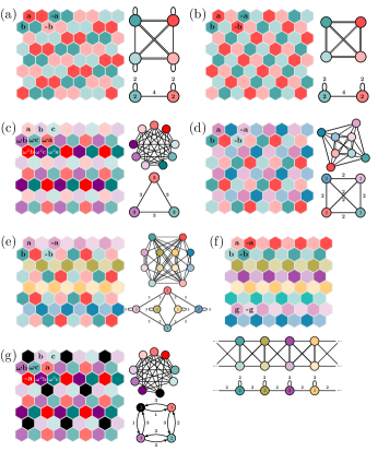
In networks of Stuart-Landau oscillators, amplitude death can coexist with the phenomena described above. For instance, if any of the nonzero amplitude splay clusters is replaced with a set of dead nodes, the state is still admissible. Additionally, we present an example illustrating a different possibility on Fig. 8 (g). The state consists of three splay clusters and a cluster of dead nodes. Two of the splay clusters are the same as those shown on Fig. 8 (c). The nodes in the third cluster of Fig. 8 (c), shown in red, form a decoupled cluster and a cluster of dead nodes on Fig. 8 (g). Two decoupled clusters are characterized by winding numbers $m_{1,2}=3$, and the third cluster has $m_{3}=2$.

In some of the patterns, all the nodes are decoupled from their own splay cluster in addition to being decoupled from all the other splay clusters. That implies the state is not linearly stable if the nodal dynamics is described by phase-only oscillator dynamics such as those of nearest neighbor Kuramoto and Kuramoto-Sakaguchi model [33].

The analysis can be extended to higher dimensional lattices, in which even more complicated decoupling patterns could be observed. Stability of these patterns could be a subject of further investigation.

It is important to perform linear stability analysis of the decoupled state because it allows predicting which parameter regions will correspond to observing that state in simulations and experiments. Here, we present the general outline of linear stability calculation for decoupled states in equations of the form of Eq. 1 for $N=\sum\limits_{i=1}^{k}n_{i}m_{i}$.

The details of the stability calculation depend on the form of nodal dynamics, the decoupled state (periodic or quasiperiodic, equal or unequal winding numbers $m_{i}$), the type of coupling (Laplacian or adjacency matrix), and the coupling topology within splay clusters. In some cases, the stability calculations can be simplified using symmetry considerations, both by block diagonalizing using subgroups of the automorphism group leading to cluster synchronization [11] and by block diagonalizing by additionally using the symmetries of the splay states [32, 33]. In other cases, symmetry methods may not be applicable.

Since the dynamics of each node correspond to two degrees of freedom, the Jacobian evaluated at the decoupled state is a $2N\times 2N$ matrix. For simplicity, we order the nodes according to the splay clusters to which they belong. The full Jacobian matrix can be written as:

$\displaystyle J=\begin{pmatrix}J_{C_{1},C_{1}}&\dots&J_{C_{1},C_{k}}\\ \vdots&\ddots&\vdots\\ J_{C_{k},C_{1}}&\dots&J_{C_{k},C_{k}}\end{pmatrix},$

(24)

where each block $J_{C_{i},C_{j}}$ of size $2m_{i}n_{i}\times 2m_{j}n_{j}$ corresponds to the interactions between the splay clusters. Furthermore, each of these blocks is of the form:

$\displaystyle J_{C_{p_{1}},C_{p_{2}}}=\begin{pmatrix}J_{C^{q_{1}}_{p_{1}},C^{q_{1}}_{p_{2}}}&\dots&J_{C^{q_{1}}_{p_{1}},C^{q_{m}}_{p_{2}}}\\ \vdots&\ddots&\vdots\\ J_{C^{q_{m}}_{p_{1}},C^{q_{1}}_{p_{2}}}&\dots&J_{C^{q_{m}}_{p_{1}},C^{q_{m}}_{p_{2}}}\end{pmatrix},$

(25)

where the finer blocks $J_{C^{q_{i}}_{p_{j}},C^{q_{k}}_{p_{l}}}$ correspond to the interactions between the fully synchronized sub-clusters. The fully synchronized sub-cluster blocks are of the form:

$\displaystyle J_{C_{p_{1}}^{q_{1}},C_{p_{2}}^{q_{2}}}=\begin{pmatrix}J_{i_{1},j_{1}}&\dots&J_{i_{1},j_{n_{2}}}\\ \vdots&\ddots&\vdots\\ J_{i_{n_{1}},j_{1}}&\dots&J_{i_{n_{1}},j_{n_{2}}}\end{pmatrix}.$

(26)

Here, $C_{p_{1}}^{q_{1}}=\{i_{1},...,i_{n_{1}}\}$, and $C_{p_{2}}^{q_{2}}=\{j_{1},...,j_{n_{2}}\}$. Finally, the Jacobian associated with each pair of oscillators is:

$\displaystyle J_{ij}=\begin{pmatrix}J_{r_{i},r_{j}}&J_{r_{i},\theta_{j}}\\ J_{\theta_{i},r_{j}}&J_{\theta_{i},\theta_{j}}\end{pmatrix}=\begin{pmatrix}\dfrac{\dot{\delta r_{i}}}{\delta r_{j}}&\dfrac{\dot{\delta r_{i}}}{\delta\theta_{j}}\\ \dfrac{\dot{\delta\theta_{i}}}{\delta r_{j}}&\dfrac{\dot{\delta\theta_{i}}}{\delta\theta_{j}}\\ \end{pmatrix},$

(27)

where $\delta r_{i}$ and $\delta\theta_{i}$ are small perturbations of the amplitude and phase of the $i$^th oscillator around the decoupled state.

For instance, if $m_{1}=...=m_{k}$, the full Jacobian $J$ is a $2N\times 2N$ matrix, where $N=(n_{1}+...+n_{k})m$. Then, for $i_{1}=\sum\limits_{j=1}^{p_{1}-1}mn_{j}+(p_{1}-1)q_{1}+r_{1}$ and $i_{2}=\sum\limits_{j=1}^{p_{2}-1}mn_{j}+(p_{2}-1)q_{2}+r_{2}$, $J_{i_{1},i_{2}}$ represents the interactions between the oscillators in $C_{p_{1}}^{q_{1}}$ and $C_{p_{2}}^{q_{2}}$ blocks.

Given a specified decoupled state, the Jacobian blocks $J_{ij}$ (where $i\in C_{p_{1}}^{q_{1}}$ and $i\in C_{p_{2}}^{q_{2}}$) on that decoupled state can be evaluated explicitly:

$\displaystyle J_{ij}$

$\displaystyle=\left\{\begin{array}[]{lr}\begin{pmatrix}{\partial f_{r_{i}}}/{\partial r_{i}}&\sum\limits_{i\in C_{p}}\kappa A_{ij}r\sin\beta\\ \sum\limits_{i\in C_{p}}\kappa A_{ij}\dfrac{1}{r}\sin\beta&\sum\limits_{i\in C_{p}}-\kappa A_{ij}\cos\beta\\ \end{pmatrix},\\ \text{for }i=j;\\ A_{ij}\kappa\begin{pmatrix}\cos(\beta+\Delta^{q_{1}q_{2}}_{p_{1}p_{2}})&-r\sin(\beta+\Delta^{q_{1}q_{2}}_{p_{1}p_{2}})\\ \dfrac{1}{r}\sin(\beta+\Delta^{q_{1}q_{2}}_{p_{1}p_{2}})&\cos(\beta+\Delta^{q_{1}q_{2}}_{p_{1}p_{2}})\end{pmatrix},\\ \text{for }i\in C^{q_{1}}_{p_{1}},j\in C^{q_{2}}_{p_{2}},\end{array}\right.$

(32)

where we assume homogeneous coupling parameters. Here, for the general quasiperiodic case in case of uniform $m$, $\Delta^{q_{1}q_{2}}_{p_{1}p_{2}}(t)=\sigma_{p_{1}p_{2}}(t)+\sigma_{q_{1}q_{2}}$, where $\sigma_{q_{1}q_{2}}=\dfrac{2\pi}{m}\times\left((q_{1}-q_{2})\mod m\right)$, and $\sigma_{p_{1}p_{2}}(t)=\sigma_{p_{1}p_{2}}(0)+\dot{\sigma}_{p_{1}p_{2}}t$ is a linearly evolving phase difference between the clusters.

If the Jacobian is time-independent, linear stability analysis can be performed by obtaining the largest real part of a Jacobian eigenvalue corresponding to transverse perturbations (as opposed to the neutrally stable perturbations of phases in the direction within the state correspond to $k$ zero eigenvalues, where $k$ is the number of splay clusters in the decoupled state). If the Jacobian is a periodic matrix (namely, only two clusters have an irrational frequency ratio), the stability analysis can be performed using Floquet theory. That is always possible when only two decoupled clusters are present. If more than two clusters are present and no special restrictions are imposed on frequencies, the Jacobian is quasiperiodic and different methods are needed to perform stability analysis.

Symmetries are extremely useful in analyzing various states of equivariant networked dynamical systems [32, 11], determining the observability and controllability of such dynamical systems [54, 55, 56], as well as studying their global behaviors via transfer operators and their numerical approximations [57]. Likewise, if the decoupled state arises from symmetries alone, these symmetries can be used to assist in stability calculations using linear representation theory as shown below. Though the case of $m_{i}\neq m_{j}$ can appear as a result of symmetries, we first focus on the case of uniform $m$. The symmetries of the Jacobian in that case are a combination of the symmetries associated with the orbital partition of the network, and the symmetries leading to the splay state. The splay state symmetries show up as follows. If $i\in C^{q_{1}}_{p_{1}}$ and $j\in C^{q_{2}}_{p_{2}}$, $k\in C^{q_{3}}_{p_{3}}$ and $l\in C^{q_{4}}_{p_{4}}$, for $\left((q_{1}-q_{2})\mod m\right)=\left((q_{3}-q_{4})\mod m\right)$ it is the case that $J_{ij}=J_{kl}$ if $A_{ij}=A_{kl}$ (in other words, the coupling within each block is defined by a circulant matrix). This simply follows from the general form of the dynamics we consider in Eq. 1. Below we present the conditions under which these symmetries (e.g., discussed in [22]) can be used to simplify the linear stability calculations.

Let $M$ be the coupling matrix, and let $\Gamma$ be the automorphism group of the matrix. The group is formed by permutation matrices $P_{\gamma}$ that act by relabeling the network nodes. Let $\Sigma_{c}\subseteq\Gamma$ be its subgroup such that its orbit partitions the nodes into decoupled splay clusters. Let $\Sigma_{s}\subset\Sigma_{c}$ be the subgroup such that its orbit partitions the nodes further into fully synchronized clusters. To obtain decoupled splay clusters of equal winding number $m$, we require $\Sigma_{c}$ (and therefore $\Sigma_{s}$) to be subgroups of $(S_{n_{1}}\times...\times S_{n_{k}})\times Z_{m}$. Additionally, we require $Z_{m}\subseteq\Sigma_{c}$. Here, $S_{n_{i}}$ refers to the symmetric group of degree $n_{i}$.

Since $\Sigma_{s}$ leads to fully synchronized clusters, it can be used to block diagonalize the Jacobian according to its isotypic components (or, equivalently, irreducible representations) [11]. The symmetries of the splay states and their effect on the structure of the Jacobian, however, can also be taken into account, and the Jacobian can be block diagonalized according to the irreducible representations of $\Sigma_{c}$ instead, leading to a finer structure [32, 33]. This results in a new coordinate system, defined by a linear transformation $T$, such that $TJT^{-1}$ is block diagonal, and thus simplifies the calculation of its associated eigenvalues (static $J$ case, periodic state) or Floquet exponents (for quasiperiodic state with linearly evolving inter-cluster phase differences). A more detailed outline of the process is presented in Appendix B.

We first consider how the considerations above can be applied to a previously discussed example of a ring of oscillators.

Next, we present how to perform this simplification for a “cube” of eight oscillators. The ring and cube networks exhibit the same decoupled state, but the stability simplification process is different.

Isotypic component decomposition is not directly applicable if the state does not appear as a result of symmetries. However, the stability analysis can still be simplified [13, 29, 58]. Here, we present a low-dimensional example where the analysis can be performed even without the extra simplifications.

We modify the network in Example V.0.2 to break the original network symmetries in a way that keeps the decoupled state admissible. The original topology is shown in Fig. 10 (g). We demonstrate these topology modifications in Fig. 10 (g^′) and Fig. 11 (g^′). The coupling topology of Fig. 10 (g^′) corresponds to adding edges between different decoupled clusters such that the inter-cluster coupling terms still add up to zero. In this setting, the decoupled state can still appear in presence of adjacency coupling. We present its stability for various parameter regimes on Fig. 10(a^′-f^′). The regions of parameter space where the state is stable are similar to those related to symmetric coupling, illustrated in Fig. 10(a-g), though the details of the stability region boundaries differ. Similarly, we expect the modified topology to modify the shape of the state’s basin of attraction once the parameters are fixed.

We also break the symmetry of the network in a way that makes the state admissible for Laplacian coupling by deleting an edge between two nodes in a fully synchronized cluster, as shown in Fig. 11 (g’). The resulting stability diagrams are shown in Fig. 11 (a^′-f^′). The stability diagrams show that symmetry breaking affects the shape of the stability regions, but preserves the possibility of observing these states in experiments, e.g., the experimental realization of networks of Stuart-Landau oscillators described in Ref. [59].

References

- [1] Peter Ashwin, Stephen Coombes, and Rachel Nicks. Mathematical frameworks for oscillatory network dynamics in neuroscience. The Journal of Mathematical Neuroscience, 6(1):2, 2016.
- [2] Kevin M Hannay, Daniel B Forger, and Victoria Booth. Macroscopic models for networks of coupled biological oscillators. Science advances, 4(8):e1701047, 2018.
- [3] James J Collins and Ian N Stewart. Coupled nonlinear oscillators and the symmetries of animal gaits. Journal of Nonlinear Science, 3(1):349–392, 1993.
- [4] Steven H Strogatz and Ian Stewart. Coupled oscillators and biological synchronization. Scientific American, 269(6):102–109, 1993.
- [5] Takashi Nishikawa and Adilson E Motter. Comparative analysis of existing models for power-grid synchronization. New Journal of Physics, 17(1):015012, 2015.
- [6] Martin Rohden, Andreas Sorge, Marc Timme, and Dirk Witthaut. Self-organized synchronization in decentralized power grids. Physical review letters, 109(6):064101, 2012.
- [7] Steven H Strogatz. From Kuramoto to Crawford: exploring the onset of synchronization in populations of coupled oscillators. Physica D: Nonlinear Phenomena, 143(1-4):1–20, 2000.
- [8] Yoshiki Kuramoto. Chemical oscillations, waves, and turbulence. Courier Corporation, 2003.
- [9] Bard Ermentrout. An adaptive model for synchrony in the firefly pteroptyx malaccae. Journal of Mathematical Biology, 29(6):571–585, 1991.
- [10] Vladimir N Belykh, Grigory V Osipov, Valentin S Petrov, Johan AK Suykens, and Joos Vandewalle. Cluster synchronization in oscillatory networks. Chaos: An Interdisciplinary Journal of Nonlinear Science, 18(3):037106, 2008.
- [11] Louis M Pecora, Francesco Sorrentino, Aaron M Hagerstrom, Thomas E Murphy, and Rajarshi Roy. Cluster synchronization and isolated desynchronization in complex networks with symmetries. Nature communications, 5:4079, 2014.
- [12] Michael T Schaub, Neave O’Clery, Yazan N Billeh, Jean-Charles Delvenne, Renaud Lambiotte, and Mauricio Barahona. Graph partitions and cluster synchronization in networks of oscillators. Chaos: An Interdisciplinary Journal of Nonlinear Science, 26(9):094821, 2016.
- [13] Francesco Sorrentino, Louis M Pecora, Aaron M Hagerstrom, Thomas E Murphy, and Rajarshi Roy. Complete characterization of the stability of cluster synchronization in complex dynamical networks. Science advances, 2(4):e1501737, 2016.
- [14] Martin Golubitsky, Ian Stewart, and David G Schaeffer. Singularities and groups in bifurcation theory, volume 2. Springer Science & Business Media, 2012.
- [15] Tommaso Menara, Giacomo Baggio, Danielle S Bassett, and Fabio Pasqualetti. Stability conditions for cluster synchronization in networks of heterogeneous kuramoto oscillators. IEEE Transactions on Control of Network Systems, 7(1):302–314, 2019.
- [16] Steven H Strogatz and Renato E Mirollo. Splay states in globally coupled Josephson arrays: Analytical prediction of Floquet multipliers. Physical Review E, 47(1):220, 1993.
- [17] Wei Zou and Meng Zhan. Splay states in a ring of coupled oscillators: From local to global coupling. SIAM Journal on Applied Dynamical Systems, 8(3):1324–1340, 2009.
- [18] Peter Ashwin and Oleksandr Burylko. Weak chimeras in minimal networks of coupled phase oscillators. Chaos: An Interdisciplinary Journal of Nonlinear Science, 25(1):013106, 2015.
- [19] Young Sul Cho, Takashi Nishikawa, and Adilson E Motter. Stable chimeras and independently synchronizable clusters. Physical review letters, 119(8):084101, 2017.
- [20] Anna Zakharova, Marie Kapeller, and Eckehard Schöll. Chimera death: Symmetry breaking in dynamical networks. Physical review letters, 112(15):154101, 2014.
- [21] Daniel M. Abrams and Steven H. Strogatz. Chimera states for coupled oscillators. Physical Review Letters, 93(17), Oct 2004.
- [22] James C Alexander and Bernold Fiedler. Global decoupling of coupled symmetric oscillators. In Differential Equations, pages 7–16, New York, 1989. Marcel Dekker Inc.
- [23] JC Alexander and Giles Auchmuty. Global bifurcations of phase-locked oscillators. Archive for Rational Mechanics and Analysis, 93(3):253–270, 1986.
- [24] Peter Ashwin and James W Swift. The dynamics of n weakly coupled identical oscillators. Journal of Nonlinear Science, 2(1):69–108, 1992.
- [25] Eric Brown, Philip Holmes, and Jeff Moehlis. Globally coupled oscillator networks. In Perspectives and Problems in Nolinear Science, pages 183–215. Springer, 2003.
- [26] Matthew H Matheny, Jeffrey Emenheiser, Warren Fon, Airlie Chapman, Anastasiya Salova, Martin Rohden, Jarvis Li, Mathias Hudoba de Badyn, Márton Pósfai, Leonardo Duenas-Osorio, et al. Exotic states in a simple network of nanoelectromechanical oscillators. Science, 363(6431):eaav7932, 2019.
- [27] Ian Stewart, Martin Golubitsky, and Marcus Pivato. Symmetry groupoids and patterns of synchrony in coupled cell networks. SIAM Journal on Applied Dynamical Systems, 2(4):609–646, 2003.
- [28] Martin Golubitsky and Ian Stewart. Synchrony versus symmetry in coupled cells. In EQUADIFF 2003, pages 13–24. World Scientific, 2005.
- [29] Abu Bakar Siddique, Louis Pecora, Joseph D Hart, and Francesco Sorrentino. Symmetry-and input-cluster synchronization in networks. Physical Review E, 97(4):042217, 2018.
- [30] Winnie Poel, Anna Zakharova, and Eckehard Schöll. Partial synchronization and partial amplitude death in mesoscale network motifs. Physical Review E, 91(2):022915, 2015.
- [31] Sanjukta Krishnagopal, Judith Lehnert, Winnie Poel, Anna Zakharova, and Eckehard Schöll. Synchronization patterns: from network motifs to hierarchical networks. Philosophical Transactions of the Royal Society A: Mathematical, Physical and Engineering Sciences, 375(2088):20160216, 2017.
- [32] Martin Golubitsky and Ian Stewart. The symmetry perspective: from equilibrium to chaos in phase space and physical space, volume 200. Springer Science & Business Media, 2003.
- [33] Jeffrey Emenheiser, Anastasiya Salova, Jordan Snyder, James P Crutchfield, and Raissa M D’Souza. Dynamically decoupled synchronization in rings of anharmonic oscillators. in preparation.
- [34] Jeffrey Emenheiser, Airlie Chapman, Márton Pósfai, James P Crutchfield, Mehran Mesbahi, and Raissa M D’Souza. Patterns of patterns of synchronization: Noise induced attractor switching in rings of coupled nonlinear oscillators. Chaos: An Interdisciplinary Journal of Nonlinear Science, 26(9):094816, 2016.
- [35] Daniel A Wiley, Steven H Strogatz, and Michelle Girvan. The size of the sync basin. Chaos: An Interdisciplinary Journal of Nonlinear Science, 16(1):015103, 2006.
- [36] Wai Lim Ku, Michelle Girvan, and Edward Ott. Dynamical transitions in large systems of mean field-coupled Landau-Stuart oscillators: Extensive chaos and cluster states. Chaos: An Interdisciplinary Journal of Nonlinear Science, 25(12):123122, 2015.
- [37] Vincent Hakim and Wouter-Jan Rappel. Dynamics of the globally coupled complex Ginzburg-Landau equation. Physical Review A, 46(12):R7347, 1992.
- [38] Seungjae Lee, Young Sul Cho, and Hyunsuk Hong. Twisted states in low-dimensional hypercubic lattices. Physical Review E, 98(6):062221, 2018.
- [39] Ron Lifshitz and MC Cross. Nonlinear dynamics of nanomechanical and micromechanical resonators. Review of nonlinear dynamics and complexity, 1:1–52, 2008.
- [40] Liudmila Tumash, Elena Panteley, Anna Zakharova, and Eckehard Schöll. Synchronization patterns in stuart–landau networks: a reduced system approach. The European Physical Journal B, 92(5):100, 2019.
- [41] Neave O’Clery, Ye Yuan, Guy-Bart Stan, and Mauricio Barahona. Observability and coarse graining of consensus dynamics through the external equitable partition. Physical Review E, 88(4):042805, 2013.
- [42] Martin Golubitsky and Ian Stewart. Rigid patterns of synchrony for equilibria and periodic cycles in network dynamics. Chaos: An Interdisciplinary Journal of Nonlinear Science, 26(9):094803, 2016.
- [43] Renato E Mirollo and Steven H Strogatz. Amplitude death in an array of limit-cycle oscillators. Journal of Statistical Physics, 60(1-2):245–262, 1990.
- [44] Fatihcan M Atay. Total and partial amplitude death in networks of diffusively coupled oscillators. Physica D: Nonlinear Phenomena, 183(1-2):1–18, 2003.
- [45] Louis M Pecora, Francesco Sorrentino, Aaron M Hagerstrom, Thomas E Murphy, and Rajarshi Roy. Discovering, constructing, and analyzing synchronous clusters of oscillators in a complex network using symmetries. In Advances in Dynamics, Patterns, Cognition, pages 145–160. Springer, 2017.
- [46] Martin Golubitsky, David Romano, and Yunjiao Wang. Network periodic solutions: full oscillation and rigid synchrony. Nonlinearity, 23(12):3227, 2010.
- [47] Martin Golubitsky, David Romano, and Yunjiao Wang. Network periodic solutions: patterns of phase-shift synchrony. Nonlinearity, 25(4):1045, 2012.
- [48] Vincenzo Nicosia, Miguel Valencia, Mario Chavez, Albert Díaz-Guilera, and Vito Latora. Remote synchronization reveals network symmetries and functional modules. Physical review letters, 110(17):174102, 2013.
- [49] Manuela AD Aguiar and Ana Paula S Dias. Synchronization and equitable partitions in weighted networks. Chaos: An Interdisciplinary Journal of Nonlinear Science, 28(7):073105, 2018.
- [50] Fernando Antoneli and Ian Stewart. Symmetry and synchrony in coupled cell networks 2: Group networks. International Journal of Bifurcation and Chaos, 17(03):935–951, 2007.
- [51] Ian Stewart and Dinis Gökaydin. Symmetries of quotient networks for doubly periodic patterns on the square lattice. International Journal of Bifurcation and Chaos, 29(10):1930026, 2019.
- [52] Yunjiao Wang and Martin Golubitsky. Two-colour patterns of synchrony in lattice dynamical systems. Nonlinearity, 18(2):631, 2004.
- [53] Constantine Pozrikidis. An introduction to grids, graphs, and networks. Oxford University Press, 2014.
- [54] Andrew J Whalen, Sean N Brennan, Timothy D Sauer, and Steven J Schiff. Observability and controllability of nonlinear networks: The role of symmetry. Physical Review X, 5(1):011005, 2015.
- [55] Michael Dellnitz and Stefan Klus. Sensing and control in symmetric networks. Dynamical Systems, 32(1):61–79, Aug 2016.
- [56] Afshin Mesbahi, Jingjing Bu, and Mehran Mesbahi. Nonlinear observability via koopman analysis: Characterizing the role of symmetry. arXiv preprint arXiv:1904.08449, 2019.
- [57] Anastasiya Salova, Jeffrey Emenheiser, Adam Rupe, James P Crutchfield, and Raissa M D’Souza. Koopman operator and its approximations for systems with symmetries. Chaos: An Interdisciplinary Journal of Nonlinear Science, 29(9):093128, 2019.
- [58] Yuanzhao Zhang and Adilson E Motter. Symmetry-independent stability analysis of synchronization patterns. arXiv preprint arXiv:2003.05461, 2020.
- [59] Baris Karakaya, Ludovico Minati, Lucia Valentina Gambuzza, and Mattia Frasca. Fading of remote synchronization in tree networks of Stuart-Landau oscillators. Physical Review E, 99(5):052301, 2019.
- [60] Yuzhen Qin, Ming Cao, Brian Anderson, Danielle S Bassett, and Fabio Pasqualetti. Mediated remote synchronization: the number of mediators matters. arXiv preprint arXiv:2003.07405, 2020.
- [61] Aaron Hagerstrom. Network symmetries and synchronization. https://sourceforge.net/projects/networksym/, 112(15):154101, 2014.