Decoupled Dynamic Filter Networks
Abstract
Convolution is one of the basic building blocks of CNN architectures. Despite its common use, standard convolution has two main shortcomings: Content-agnostic and Computation-heavy. Dynamic filters are content-adaptive, while further increasing the computational overhead. Depth-wise convolution is a lightweight variant, but it usually leads to a drop in CNN performance or requires a larger number of channels. In this work, we propose the Decoupled Dynamic Filter (DDF) that can simultaneously tackle both of these shortcomings. Inspired by recent advances in attention, DDF decouples a depth-wise dynamic filter into spatial and channel dynamic filters. This decomposition considerably reduces the number of parameters and limits computational costs to the same level as depth-wise convolution. Meanwhile, we observe a significant boost in performance when replacing standard convolution with DDF in classification networks. ResNet50 / 101 get improved by 1.9 and 1.3 on the top-1 accuracy, while their computational costs are reduced by nearly half. Experiments on the detection and joint upsampling networks also demonstrate the superior performance of the DDF upsampling variant (DDF-Up) in comparison with standard convolution and specialized content-adaptive layers. The project page with code is available111https://thefoxofsky.github.io/project_pages/ddf.
1 Introduction
Convolution is a fundamental building block of convolutional neural networks (CNNs) that have seen tremendous success in several computer vision tasks, such as image classification, semantic segmentation, pose estimation, to name a few. Thanks to its simple formulation and optimized implementations, convolution has become a de facto standard to propagate and integrate features across image pixels. In this work, we aim to alleviate two of its main shortcomings: Content-agnostic and Computation-heavy.

Content-agnostic. Spatial-invariance is one of the prominent properties of a standard convolution. That is, convolution filters are shared across all the pixels in an image. Consider the sample road scene shown in Figure 1 (top). The convolution filters are shared across different regions such as buildings, cars, roads, etc. Given the varied nature of contents in a scene, a spatially shared filter may not be optimal to capture features across different image regions [52, 42]. In addition, once a CNN is trained, the same convolution filters are used across different images (for instance images taken in daylight and at night). In short, standard convolution filters are content-agnostic and are shared across images and pixels, leading to sub-optimal feature learning. Several existing works [23, 48, 42, 57, 49, 45, 22, 11] propose different types of content-adaptive (dynamic) filters for CNNs. However, these dynamic filters are either compute-intensive [57, 23], memory-intensive [42, 22], or specialized processing units [11, 48, 49, 45]. As a result, most of the existing dynamic filters can not completely replace standard convolution in CNNs and are usually used as a few layers of a CNN [49, 45, 42, 22], or in tiny architecture [57, 23], or in specific scenarios, like upsampling [48].
Computation-heavy. Despite the existence of highly-optimized implementations, the computation complexity of standard convolution still increases considerably with the enlarge in the filter size or channel number. This poses a significant problem as convolution layers in modern CNNs have a large number of channels in the orders of hundreds or even thousands. Grouped or depth-wise convolutions are commonly used to reduce the computation complexity. However, these alternatives usually result in CNN performance drops when directly used as a drop-in replacement to standard convolution. To retain similar performance with depth-wise or grouped convolutions, we need to considerably increase the number of feature channels, leading to more memory consumption and access times.
In this work, we propose the Decoupled Dynamic Filter (DDF) that simultaneously addresses both the above-mentioned shortcomings of the standard convolution layer. The full dynamic filter [57, 23, 49, 45] uses a separate network branch to predict a complete convolution filter at each pixel. See Figure 1 (middle) for an illustration. We observe that this dynamic filtering is equivalent to applying attention on unfolded input features, as illustrated in Figure 3. Inspired by the recent advances in attention mechanisms that apply spatial and channel-wise attention [36, 50], we propose a new variant of the dynamic filter where we decouple spatial and channel filters. In particular, we adopt separate attention-style branches that individually predict spatial and channel dynamic filters, which are then combined to form a filter at each pixel. See Figure 1 (bottom) for an illustration of DDF. We observe that this decoupling of the dynamic filter is efficient yet effective, making DDF to have similar computational costs as depth-wise convolution while achieving better performance against existing dynamic filters. This lightweight nature enables DDF to be directly inserted as a replacement of the standard convolution layer. Unlike several existing dynamic filtering layers, we can replace all convolutions in a CNN with DDF. We also propose a variant of DDF, called DDF-Up, that can be used as a specialized upsampling or joint-upsampling layer.
We empirically validate the performance of DDF by drop-in replacing convolution layers in several classification networks with DDF. Experiments indicate that applying DDF consistently boosts the performance while reducing computational costs. In addition, we also demonstrate the superior upsampling performance of DDF-Up in object detection and joint upsampling networks. In summary, DDF and DDF-Up have the following favorable properties:
-
•
Content-adaptive. DDF provides spatially-varying filtering that makes filters adaptive to image contents.
-
•
Fast runtime. DDF has similar computational costs as depth-wise convolution, so its inference speed is faster than both standard convolution and dynamic filters.
-
•
Smaller memory footprint. DDF significantly reduces memory consumption of dynamic filters, making it possible to replace all standard convolution layers with DDF.
-
•
Consistent performance improvements. Replacing a standard convolution with DDF / DDF-Up results in consistent improvements and achieves the state-of-the-art performance across various networks and tasks.
2 Related Work
Lightweight convolutions. Given the prominence of convolutions in CNN architectures, several lightweight variants have been proposed for different purposes. Dilated convolutions [4, 56] increase the receptive field of the filter without increasing parameters or computation complexity of the standard convolution. Several lightweight mobile networks [17, 39, 16] use depth-wise convolutions instead of standard ones, which separately convolve each channel. Similarly, grouped convolutions [26] group input channels and convolve each group separately resulting in parameter and computation reduction. However, directly replacing a standard convolution with depth-wise or grouped convolutions usually leads to performance drops. One needs to widen the model to achieve competitive performance with these lightweight variants of convolution. In contrast, the proposed DDF layer can be directly used as a lightweight drop-in replacement to standard convolution layer.

Dynamic filters. For the dynamic filters, the filter neighborhoods and/or filter values are dynamically modified or predicted based on the input features. Some recent approaches dynamically adjust the filter neighborhoods by adaptive dilation factors [58], estimating the neighborhood sampling grid [8], or adapting the receptive fields [43]. Another kind of dynamic filters, more closely related to our work, adjusts or predicts filter values based on input features [55, 59, 5, 23, 48, 42, 57, 49, 45, 22]. In particular, semi-dynamic filters, such as WeightNet [34], CondConv [55], DyNet [59], and DynamicConv [5], predict coefficients to combine several expert filters. The combined filter is still applied in a convolutional manner (spatially shared). CARAFE [48] proposes a dynamic layer for upsampling, where an additional network branch is used to predict a 2D filter at each pixel. However, these channel-wise shared 2D filters cannot encode channel-specific information. Several full dynamic filters [23, 57, 49, 45] use separate network branches to predict a complete filter at each pixel. As illustrated in Figure 2 (middle) and briefly explained in the Introduction, these dynamic filters can only replace a few convolution layers or can only be used in small networks due to computational reasons. Specifically, adaptive convolutional kernels [57] are only used in small networks. SOLOv2 [49] and CondInst [45] employ dynamic filters in the last few layers of the segmentation model. PAC [42] uses a fixed Gaussian kernel on adapting features to modify the standard convolution filter at each pixel, which is also impractical for large architectures due to high memory consumption. The proposed DDF is lightweight even compared with the standard convolution layer and thus can be used across all the layers even in large networks.
Attention mechanisms. Inspired by the role of attention in human visual perception [21, 38, 7, 50], several approaches [54, 47, 46, 18, 36, 50] propose to use attention layers that dynamically enhance/suppress feature values with predicted attention maps. SMemVQA [54] generates question-guided spatial attention to capture the correspondence between individual words in the question and image regions. The residual attention network [47] adopts encoder-decoder branches to model spatial attention and refine features. VSGNet [46] leverages the spatial configuration of human-object pairs to model attention. Besides spatial attention, SENet [18] introduces the squeeze-and-excitation structure to encode channel-wise attention and re-weights the feature channels. Subsequent methods combine spatial and channel-wise attention. BAM [36] uses spatial and channel-wise attention in parallel, whereas CBAM [50] sequentially applies spatial and channel-wise attention. In this work, we draw connections between dynamic filters and attention layers. Inspired by spatial and channel-wise attention, we propose DDF that uses decoupled spatial and channel dynamic filters.
3 Preliminaries
Standard convolution. Given an input feature representation with channels and pixels (, and are the width and height of the feature map); the standard convolution operation at pixel can be written as a linear combination of input features around pixel:
| (1) |
where denotes the feature vector at pixel; denotes output feature map with denoting pixel output feature vector. denotes the convolution window around pixel. is a convolution filter, is the filter at position offset between and pixels: where denotes 2D pixel coordinates. denotes the bias vector. In standard convolution, the same filter is shared across all pixels and filter weights are agnostic to input features.
Dynamic filters. In contrast to standard convolution, dynamic filters leverage separate network branches to generate the filter at each pixel. The spatially-invariant filter in Eq. 1 becomes the spatially-varying filter in this case. The dynamic filters enable learning content-adaptive and flexible feature embeddings. However, predicting such a large number () of pixel-wise filter values requires heavy side-networks, resulting in both compute and memory intensive network architectures. Thus, dynamic filters are usually only employed in either tiny networks [23, 57] or can only replace a few standard convolution layers [49, 45, 42, 22] in a CNN.
4 Decoupled Dynamic Filter
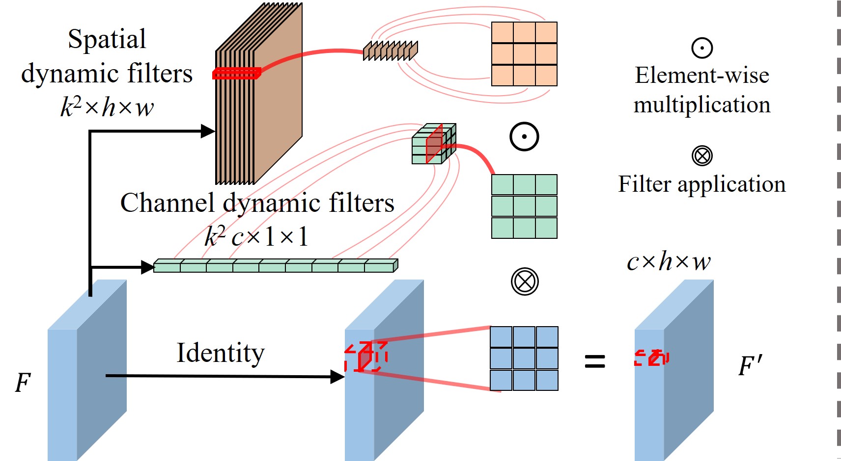
The goal of this work is to design a filtering operation that is content-adaptive while being lighter-weight than a standard convolution. Realizing both the properties with a single filter is quite challenging. We accomplish this with our Decoupled Dynamic Filter (DDF), where the key technique is to decouple dynamic filters into spatial and channel ones. More formally, the DDF operation can be written as:
| (2) |
where denotes the output feature value at the pixel and channel, denotes the input feature value at the pixel and channel. is the spatial dynamic filter with denoting the filter at pixel. is the channel dynamic filter with denoting the filter at channel. Figure 2(a) shows the illustration of DDF operation. We predict both channel and spatial dynamic filters from the input feature, using which we perform the above DDF operation (Eq. 2) to compute the output feature map. Comparing general dynamic filters (See Section 3) with DDF clearly indicates that DDF reduces the sized dynamic filter into much smaller spatial and channel dynamic filters. In addition, we implement DDF operation in CUDA alleviating any need to save intermediate multiplied filters during network training and inference.

DDF module. Based on DDF operation, we carefully design a DDF module that can act as a basic building block in CNNs. For that, we want the filter prediction branches to be lightweight as well in addition to the DDF operation itself. We notice the connection between dynamic filters and attention mechanisms, using which we design attention-style branches to predict spatial and channel filters. Figure 3 illustrates the connection between dynamic filters and attention. Applying dynamic filters on a feature map is equivalent to applying attention on unfolded features. That is, we unfold the feature map into feature map where neighboring feature values are unfolded as separate channels. Applying dynamic filters on the original feature map is the same as re-weighting the unfolded feature map using the generated filter tensor as attention.
Following the recent advances in attention literature [36, 50] that propose to use lightweight branches to predict spatial and channel-wise attention, we design two attention-style branches that can generate spatial and channel dynamic filters for DDF. Figure 2(b) illustrates the structure of spatial and channel filter branches in the DDF module. The spatial filter branch only contains one convolution layer. The channel filter branch first applies the global average pooling to aggregate input features, then generates channel dynamic filters via a squeeze-and-excitation structure [18], where the squeeze ratio is denoted as .
As generated filter values can be extremely large or small for some input features, directly using them for convolution will make the training unstable. So, we propose to do filter normalization (FN):
| (3) |
where are the generated spatial and channel filters before normalization, and calculate the mean and standard deviation of the filter, are the running standard deviation and mean values which are similar to those coefficients in the batch normalization (BN) [20]. FN can limit generated filter values into a reasonable range, thereby avoiding the gradient vanishing/exploding during training.
4.1 Computational Complexity.
Table 1 shows the parameter, space and time complexity comparisons between standard convolution (Conv), Depth-wise convolution (DwConv), full dynamic filters (DyFilter) [23, 57, 49, 45], and our DDF filter. For analysis, we use the same notation as before - Number of pixels; : Channel number; Filter size (spatial extent); Squeeze ratio in DDF channel filter branch. For simplicity, we assume that both input and output features have channels. We also assume that DyFilter adopts a lightweight filter prediction branch with a single convolution layer.
Number of parameters. The prediction branch of DyFilter takes channel features as input and produces channel output, where each pixel output corresponds to a complete filter at that pixel. Thus, the DyFilter prediction branch has parameters, which is quite high even for small values of . For DDF, the spatial filter branch predicts filter tensors with channels and thus contain parameters. The channel filter branch has parameters for the squeeze layer, and parameters for the excitation layer. In total, DDF prediction branches contain parameters, which is far fewer than those for DyFilter. Depending on the values of , , and (usually set to 0.2, 3, and 256), the number of parameters for the DDF module can be even lower than a standard convolution layer.
Time complexity. The spatial filter generation of DDF needs floating-point operations (FLOPs), and the channel filter generation takes FLOPs. The filter combination and application needs FLOPs. In total, DDF needs FLOPs with time complexity of . The term can be ignored since . Thus, the time complexity of DDF approximately equals to , which is similar to that of depth-wise convolution and better than a standard convolution with time complexity of . The time complexity of DyFilter is , with FLOPs for filter generation and FLOPs for filter application. Thus the time complexity of DyFilter is almost times higher than that of DDF, which is quite significant. Table 2 compares the inference time between four kinds of filters, where we adopt PAC [42] as the representative of dynamic filters. Refer to the supplementary for more latency comparisons on different input sizes.
| Filter | Conv | DwConv | DyFilter | DDF |
|---|---|---|---|---|
| Params | ||||
| Time | ||||
| Space | – | – |
| Filter | Conv | DwConv | PAC | DDF |
|---|---|---|---|---|
| Memory | 356.3M | 236.0M | 3406.4M | 245.7M |
| Latency | 7.5 ms | 1.0 ms | 46.4 ms | 3.0 ms |
Space/Memory complexity. Table 1 also compares the space complexity of generated filters. Standard and depth-wise convolutions do not generate content-adaptive filters. DyFilter generates a complete filter at each pixel with a space complexity of . DDF has a much smaller space complexity of , since it only needs to store 2d spatial filters with (shared by channels) and channel filters with . See Table 2 for the comparison of the max allocated memory between four kinds of filters.
In summary, DDF has a time complexity that is similar to depth-wise convolution, which is considerably better than a standard convolution or dynamic filter. Remarkably, despite generating content-adaptive filters, the number of parameters in a DDF module is still smaller than that of a standard convolution layer. The space complexity of DDF can be hundreds or even thousands of times smaller than full dynamic filters, when or are in the orders of hundreds which is quite common in practice.
5 DDF Networks for Image Classification
Image classification is considered as a fundamental task in computer vision. To demonstrate the use of DDFs as basic building blocks in a CNN, we experiment with the widely used ResNet [15] architecture for image classification. ResNets stack multiple basic/bottleneck blocks in which convolution layers are adopted for spatial embedding. We substitute these convolution layers in all stacked blocks with DDF. We refer to such a modified ResNet with DDF as ‘DDF-ResNet’. Figure 4 illustrates the use of DDF in a ResNet bottleneck block, we refer to it as DDF bottleneck block.

We evaluate DDF-ResNets on the ImageNet dataset [10] with the Top-1 and Top-5 accuracy. DDF-ResNets are trained using the same training protocol as [27]. In particular, we train models for 120 epochs by the SGD optimizer with the momentum of 0.9 and the weight decay of 1e-4. The learning rate is set to 0.1 with batch size 256 and decays to 1e-5 following the cosine schedule. The input image is resized and center-cropped to .
Ablation study. We comprehensively analyze the effect of different components in a DDF module. We choose ResNet50 [15] as our base network architecture and experiment with different modifications to DDF. Table 4(c) shows the results of ablation experiments. First, we analyze the effect of spatial and channel dynamic filters in DDF with classification accuracy. Table 4(a) shows there is a significant drop in performance when we replace convolutions with only spatial dynamic filters. This is expected as spatial dynamic filters are shared by all channels, thus cannot encode channel-specific information.
By replacing the convolution with the channel dynamic filters, the top-1 accuracy is improved by 1.6%. Using the full DDF module, with both spatial and channel dynamic filters, improves the top-1 accuracy by 1.9%. These results show the importance of both the spatial and channel dynamic filters in DDF.
Table 4(b) compares different normalization schemes in a DDF module. Replacing the proposed filter normalization with a standard batch normalization [20] or a sigmoid activation leads to considerable drops in accuracy. Sigmoid activation individually processes each filter value and may not capture the correlation between them, while batch normalization considers all the filters in a batch, which may weaken the filter dynamics across samples.
We also evaluate DDF under different squeeze ratios , which is used to control the feature channel compression in the channel filter branch. As shown in table 4(c), using higher squeeze ratios will significantly increase the number of parameters, while only bringing marginal performance improvements. Hence, we set the squeeze ratio to 0.2 by default. In addition, even the parameter number increases with enlarging the squeeze ratio, the FLOPs remain low because the computational costs of the channel filter branch are minimal, as analyzed in Section 4.1.
| Spatial | Channel | Top-1 / Top-5 Acc. |
|---|---|---|
| Base Model | 77.2 / 93.5 | |
| 74.4 / 92.0 | ||
| 78.7 / 94.2 | ||
| 79.1 / 94.5 | ||
| Batch-Norm | Sigmoid | Filter-Norm | |
| Top-1 Acc. | 76.0 | 78.2 | 79.1 |
| Top-5 Acc. | 92.0 | 93.8 | 94.5 |
| Params | FLOPs | Top-1 / Top-5 Acc | |
|---|---|---|---|
| 0.2 | 16.8M | 2.298B | 79.1 / 94.5 |
| 0.3 | 18.1M | 2.299B | 79.0 / 94.5 |
| 0.4 | 19.4M | 2.300B | 79.2 / 94.5 |
| Arch | Conv Type | Params | FLOPs | Top-1 Acc |
|---|---|---|---|---|
| R18 | Base Model [15] | 11.7M | 1.8B | 69.6 |
| Adaptive [57] | 11.1M | – | 70.2 | |
| DyNet [59] | 16.6M | 0.6B | 69.0 | |
| DDF | 7.7M | 0.4B | 70.6 | |
| R50 | Base Model [15] | 25.6M | 4.1B | 77.2 |
| DyNet [59] | – | 1.1B | 76.3 | |
| CondConv [55] | 104.8M | 4.2B | 78.6 | |
| DwCondConv [55] | 14.5M | 2.3B | 78.3 | |
| DwWeightNet [34] | 14.4M | 2.3B | 78.0 | |
| DDF | 16.8M | 2.3B | 79.1 |
| Method | Params | FLOPs | Top-1 Acc |
|---|---|---|---|
| ResNet50 (base) [15] | 25.6M | 4.1B | 76.0 (77.2) |
| SE-ResNet50 [18] | 28.1M | 4.1B | 77.6 (77.8) |
| BAM-ResNet50 [36] | 25.9M | 4.2B | 76.0 |
| CBAM-ResNet50 [50] | 28.1M | 4.1B | 77.3 |
| AA-ResNet50 [2] | 25.8M | 4.2B | 77.7 |
| ResNeXt50 (324d) [53] | 25.0M | 4.3B | 77.8 (78.2) |
| Res2Net50 (14w-8s) [12] | 25.7M | 4.2B | 78.0 |
| DDF-ResNet50 | 16.8M | 2.3B | 79.1 |
| ResNet101 (base) [15] | 44.5M | 7.8B | 77.6 (78.9) |
| SE-ResNet101 [18] | 49.3M | 7.8B | 78.3 (79.3) |
| BAM-ResNet101 [50] | 44.9M | 7.9B | 77.6 |
| CBAM-ResNet101 [50] | 49.3M | 7.8B | 78.5 |
| AA-ResNet101 [2] | 45.4M | 8.1B | 78.7 |
| ResNeXt101 (324d) [53] | 44.2M | 8.0B | 78.8 (79.5) |
| Res2Net101 (26w-4s) [12] | 45.2M | 8.1B | 79.2 |
| DDF-ResNet101 | 28.1M | 4.1B | 80.2 |
Comparisons with other dynamic filters. Next, we compare the use of DDF with respect to some existing dynamic filters using different ResNet base architectures: ResNet18 (R18) and ResNet50 (R50). Table 4 shows the parameters, FLOPs, and accuracy comparisons. Specifically, we compare DDF with adaptive convolutional kernel [57] (Adaptive), DyNet [59], Conditionally parameterized convolutions (CondConv/DwCondConv) [55], and depth-wise WeightNet (DwWeightNet) [34]. The ‘Adaptive’ [57] can only be used in R18 due to its large running memory consumption. Results show that using DDF consistently boosts the performance of base models, while also significantly reducing the number of parameters and FLOPs. It is worth noting that, DwWeightNet has worse performance than DDF, and even inferior to the channel-only DDF in Table 4(a), although it has a similar design as the channel-only DDF. This is due to the use of sigmoid activation during the filter generation in DwWeightNet
(more analysis in the supplementary).
Comparisons with state-of-the-art ResNet variants. We also compare DDF-ResNets with other state-of-the-art variants of ResNet50 and ResNet101 architectures in Table 5. Specifically, we compare with attention mechanisms of SE [18], BAM [36], CBAM [50] and AA [2]; and also block modifications of ResNeXt [53] and Res2Net [12]. Results clearly show that DDF-ResNets achieve the best performance while also having the lowest number of parameters and FLOPs. DDF-ResNet50 can be further improved by tricks in training and evaluation, and can achieve 81.3% top-1 accuracy. Refer to the supplementary for more details.
6 DDF as Upsampling Module


An advantage of dynamic filters compared with standard convolution is that one could predict dynamic filters from guidance features instead of input features. Following this, we propose an extension of the DDF module, where spatial dynamic filters are predicted using separate guidance features instead of input features. Such joint filtering with input and guidance features is useful for several tasks such as joint image upsampling [42, 28, 29], cross-modal image enhancement [51, 9, 6], texture removal [32] to name a few. Figure 5 illustrates the DDF Upsampling (DDF-Up) module, where the number of DDF operations used is set to for the upsampling factor (e.g., 4 DDF operations when the upsampling factor is 2). We stack and pixel-shuffle [40] the resulting features from the DDF operations to form output features. For typical upsampling (without guidance), we use the same structure with a slight modification. We compute guidance features from input ones using a depth-wise convolution layer. DDF-Up can be seamlessly integrated into several existing CNNs, where typical/joint upsampling operators are needed. Here we present two applications in object detection and joint depth upsampling tasks.
| Method | FLOPs | mApS | mApM | mApL | mAp |
|---|---|---|---|---|---|
| Nearest (base) | 0.00B | 21.2 | 41.0 | 48.1 | 37.4 |
| Bilinear | 0.02B | 22.1 | 41.2 | 48.4 | 37.6 |
| Deconv [35] | 12.57B | 21.0 | 41.1 | 48.5 | 37.3 |
| P.S. [40] | 50.18B | 21.4 | 41.5 | 48.6 | 37.7 |
| CARAFE [48] | 2.14B | 22.6 | 42.0 | 49.8 | 38.5 |
| DDF-Up | 0.58B | 22.1 | 42.4 | 49.9 | 38.6 |
Object detection with DDF-Up. Detecting objects in an image is one of the core dense prediction tasks in computer vision. We adopt FasterRCNN [37] with the Feature Pyramid Network (FPN) [30] as our base detection architecture and embed DDF-Up modules into FPN. FPN is an effective U-net shaped feature fusion module, where the decoder pathway upsamples high-level features while combining low-level ones. As illustrated in Figure 6(a), we replace the nearest-neighbor upsampling modules in FPN with our DDF-Up modules.

|

|

|

|

|

|

|

|

|

|

|

|
| Input | Guidance | Bilinear | PAC-Net [42] | DDF-Up-Net (Ours) | GT |
We analyze the effectiveness of DDF-Up modules with experiments on the COCO detection benchmark [31] which contains 115K training and 5K validation images. We report standard COCO [31] metrics for small (mApS), medium (mApM), large (mApL), and all-scale (mAp) objects on the minival split. We implement our models based on the MMDetection [3] toolbox and train them using the standard training protocol therein. Specifically, we train different models for 12 epochs using the SGD optimizer with a momentum of 0.1 and the weight decay of 1e-4. We use a batch size of 16 and set the learning rate to 0.2 which decays by the factor of 0.1 at 8 and 11th epochs. We resize the shorter side of the input image to 800 pixels, while keeping the longer side no larger than 1333 pixels.
We compare DDF-Up with the generic nearest-neighbor (Nearest) and bilinear (Bilinear) interpolations, as well as learnable Deconvolution (Deconv) [35], Pixel Shuffle (P.S.) [40], and CARAFE [48] upsampling modules. Table 6 exhibits the comparison results. FPN with DDF-Up yields a 1.2% mAp improvement over the baseline which adopts the nearest-neighbor interpolation. DDF-Up also brings obvious improvements against static-filtering upsampler (like Deconv and P.S.), and is on par with the recent dynamic upsampling technique CARAFE while utilizing only one-third of FLOPs as CARAFE.
Joint depth upsampling with DDF-Up. We analyze the use of DDF-Up as a joint upsampling module by integrating it into a joint depth upsampling network. Here, the task is to upsample a low-resolution depth map given a higher-resolution RGB image as guidance. This experiment allows to compare DDF-Up with content-adaptive filtering techniques such as Pixel-Adaptive Convolution (PAC) [42] which is a current state-of-the-art for this task. We use a similar network architecture to PAC-Net [42], where we employ our DDF-Up modules instead of PAC joint upsampling modules. We call the resulting network ‘DDF-Up-Net’. Figure 6(b) illustrates DDF-Up-Net where we first encode low-resolution input features from the given depth map () and high-resolution guidance features () from RGB images. Then, we employ DDF-Up in the decoder to joint upsample depth features with guidance features and obtain high-resolution depth output (). Each DDF-Up module does upsampling, we sequentially use DDF-Up modules when the upsampling factor is .
We conduct experiments on the NYU depth V2 dataset [41] which has 1449 RGB-depth pairs. Following PAC-Net [42], we use the nearest-neighbor downsampling to generate low-resolution inputs from the ground-truth (GT) depth maps. We split the first 1000 samples for training and the rest for testing. We train DDF-Up-Net for 1500 epochs using the Adam optimizer [24]. We use a batch size of 8 and set the learning rate to 1e-4 which decays by the factor 0.1 at 1000 and 1350th epochs. During training, the input images are resized and random-cropped to . Table 7 reports Root Mean Square Error (RMSE) scores of different techniques for three upsampling factors, \ie, , , and . DDF-Up-Net performs better than state-of-the-art techniques across all the upsampling factors. It surpasses the standard CNN techniques like DJF [28] and DJF+ [29] by a large margin. It also improves over dynamic-filtering PAC [42] while reducing computational costs by an order of magnitude. See Table 2 for the cost comparison between PAC and DDF-Up. We visualize sampled 16 upsampling results in Figure 7, where we can see that DDF-Up-Net recovers more details compared to PAC-Net and other techniques.
| Method | 4 | 8 | 16 |
|---|---|---|---|
| Bicubic | 8.16 | 14.22 | 22.32 |
| MRF (324d) | 7.84 | 13.98 | 22.20 |
| GF [14] | 7.32 | 13.62 | 22.03 |
| Ham et al. [13] | 5.27 | 12.31 | 19.24 |
| FBS [1] | 4.29 | 8.94 | 14.59 |
| JBU [25] | 4.07 | 8.29 | 13.35 |
| DMSG [19] | 3.78 | 6.37 | 11.16 |
| DJF [28] | 3.54 | 6.20 | 10.21 |
| DJF+ [29] | 3.38 | 5.86 | 10.11 |
| PAC-Net [42] | 2.39 | 4.59 | 8.09 |
| DDF-Up-Net | 2.16 | 4.40 | 7.72 |
7 Conclusion
In this work, we propose a lightweight content-adaptive filtering technique called DDF, where our key strategy is to predict decoupled spatial and channel dynamic filters. We show that DDF can seamlessly replace standard convolution layers, consistently improving the performance of ResNets while also reducing model parameters and computational costs. In addition, we propose an upsampling variant called DDF-Up, which boosts performance as both a general upsampling module in detection and a joint upsampling module in joint depth upsampling. DDF-Up also is more computationally efficient compared with specialized content-adaptive layers. Overall, DDF has rich representative capabilities as a content-adaptive filter while also being computationally cheaper than a standard convolution, making it highly practical to use in modern CNNs.
8 Acknowledgement
This work is supported in part by the National Natural Science Foundation of China (No.61976094). M.-H. Yang is supported in part by NSF CAREER 1149783.
References
- [1] Jonathan T Barron and Ben Poole. The fast bilateral solver. In ECCV, 2016.
- [2] Irwan Bello, Barret Zoph, Ashish Vaswani, Jonathon Shlens, and Quoc V Le. Attention augmented convolutional networks. In ICCV, 2019.
- [3] Kai Chen, Jiaqi Wang, Jiangmiao Pang, Yuhang Cao, Yu Xiong, Xiaoxiao Li, Shuyang Sun, Wansen Feng, Ziwei Liu, Jiarui Xu, Zheng Zhang, Dazhi Cheng, Chenchen Zhu, Tianheng Cheng, Qijie Zhao, Buyu Li, Xin Lu, Rui Zhu, Yue Wu, Jifeng Dai, Jingdong Wang, Jianping Shi, Wanli Ouyang, Chen Change Loy, and Dahua Lin. MMDetection: Open mmlab detection toolbox and benchmark. arXiv preprint arXiv:1906.07155, 2019.
- [4] Liang-Chieh Chen, George Papandreou, Iasonas Kokkinos, Kevin Murphy, and Alan L Yuille. Deeplab: Semantic image segmentation with deep convolutional nets, atrous convolution, and fully connected crfs. IEEE Transactions on Pattern Analysis and Machine Intelligence, 40(4):834–848, 2017.
- [5] Yinpeng Chen, Xiyang Dai, Mengchen Liu, Dongdong Chen, Lu Yuan, and Zicheng Liu. Dynamic convolution: Attention over convolution kernels. In CVPR, 2020.
- [6] Yukyung Choi, Namil Kim, Soonmin Hwang, Kibaek Park, Jae Shin Yoon, Kyounghwan An, and In So Kweon. Kaist multi-spectral day/night data set for autonomous and assisted driving. IEEE Transactions on Intelligent Transportation Systems, 2018.
- [7] Maurizio Corbetta and Gordon L Shulman. Control of goal-directed and stimulus-driven attention in the brain. Nature Reviews Neuroscience, 2002.
- [8] Jifeng Dai, Haozhi Qi, Yuwen Xiong, Yi Li, Guodong Zhang, Han Hu, and Yichen Wei. Deformable convolutional networks. In ICCV, 2017.
- [9] Pingyang Dai, Rongrong Ji, Haibin Wang, Qiong Wu, and Yuyu Huang. Cross-modality person re-identification with generative adversarial training. In IJCAI, 2018.
- [10] Jia Deng, Wei Dong, Richard Socher, Li-Jia Li, Kai Li, and Li Fei-Fei. Imagenet: A large-scale hierarchical image database. In CVPR, 2009.
- [11] Raghudeep Gadde, Varun Jampani, Martin Kiefel, Daniel Kappler, and Peter V Gehler. Superpixel convolutional networks using bilateral inceptions. In ECCV, 2016.
- [12] Shanghua Gao, Ming-Ming Cheng, Kai Zhao, Xin-Yu Zhang, Ming-Hsuan Yang, and Philip HS Torr. Res2net: A new multi-scale backbone architecture. IEEE Transactions on Pattern Analysis and Machine Intelligence, 2019.
- [13] Bumsub Ham, Minsu Cho, and Jean Ponce. Robust image filtering using joint static and dynamic guidance. In CVPR, 2015.
- [14] Kaiming He, Jian Sun, and Xiaoou Tang. Guided image filtering. In ECCV, 2010.
- [15] Kaiming He, Xiangyu Zhang, Shaoqing Ren, and Jian Sun. Deep residual learning for image recognition. In CVPR, 2016.
- [16] Andrew Howard, Mark Sandler, Grace Chu, Liang-Chieh Chen, Bo Chen, Mingxing Tan, Weijun Wang, Yukun Zhu, Ruoming Pang, Vijay Vasudevan, et al. Searching for mobilenetv3. In ICCV, 2019.
- [17] Andrew G Howard, Menglong Zhu, Bo Chen, Dmitry Kalenichenko, Weijun Wang, Tobias Weyand, Marco Andreetto, and Hartwig Adam. Mobilenets: Efficient convolutional neural networks for mobile vision applications. arXiv preprint arXiv:1704.04861, 2017.
- [18] Jie Hu, Li Shen, and Gang Sun. Squeeze-and-excitation networks. In CVPR, 2018.
- [19] Tak-Wai Hui, Chen Change Loy, and Xiaoou Tang. Depth map super-resolution by deep multi-scale guidance. In ECCV, 2016.
- [20] Sergey Ioffe and Christian Szegedy. Batch normalization: Accelerating deep network training by reducing internal covariate shift. ICML, 2015.
- [21] Laurent Itti, Christof Koch, and Ernst Niebur. A model of saliency-based visual attention for rapid scene analysis. IEEE Transactions on Pattern Analysis and Machine Intelligence, 1998.
- [22] Varun Jampani, Martin Kiefel, and Peter V Gehler. Learning sparse high dimensional filters: Image filtering, dense crfs and bilateral neural networks. In CVPR, pages 4452–4461, 2016.
- [23] Xu Jia, Bert De Brabandere, Tinne Tuytelaars, and Luc V Gool. Dynamic filter networks. In NeurIPS, 2016.
- [24] Diederik P Kingma and Jimmy Ba. Adam: A method for stochastic optimization. ICLR, 2015.
- [25] Johannes Kopf, Michael F Cohen, Dani Lischinski, and Matt Uyttendaele. Joint bilateral upsampling. ACM Transactions on Graphics, 2007.
- [26] Alex Krizhevsky, Ilya Sutskever, and Geoffrey E Hinton. Imagenet classification with deep convolutional neural networks. In NeurIPS, 2012.
- [27] Duo Li, Anbang Yao, and Qifeng Chen. Psconv: Squeezing feature pyramid into one compact poly-scale convolutional layer. In ECCV, 2020.
- [28] Yijun Li, Jia-Bin Huang, Narendra Ahuja, and Ming-Hsuan Yang. Deep joint image filtering. In ECCV, 2016.
- [29] Yijun Li, Jia-Bin Huang, Narendra Ahuja, and Ming-Hsuan Yang. Joint image filtering with deep convolutional networks. IEEE Transactions on Pattern Analysis and Machine Intelligence, 2019.
- [30] Tsung-Yi Lin, Piotr Dollár, Ross Girshick, Kaiming He, Bharath Hariharan, and Serge Belongie. Feature pyramid networks for object detection. In CVPR, 2017.
- [31] Tsung-Yi Lin, Michael Maire, Serge Belongie, James Hays, Pietro Perona, Deva Ramanan, Piotr Dollár, and C Lawrence Zitnick. Microsoft coco: Common objects in context. In ECCV, 2014.
- [32] Feng Liu and Michael Gleicher. Texture-consistent shadow removal. In ECCV, 2008.
- [33] Hanxiao Liu, Karen Simonyan, and Yiming Yang. Darts: Differentiable architecture search. ICLR, 2019.
- [34] Ningning Ma, Xiangyu Zhang, Jiawei Huang, and Jian Sun. Weightnet: Revisiting the design space of weight networks. In ECCV, 2020.
- [35] Hyeonwoo Noh, Seunghoon Hong, and Bohyung Han. Learning deconvolution network for semantic segmentation. In ICCV, 2015.
- [36] Jongchan Park, Sanghyun Woo, Joon-Young Lee, and In So Kweon. Bam: Bottleneck attention module. BMVC, 2018.
- [37] Shaoqing Ren, Kaiming He, Ross Girshick, and Jian Sun. Faster r-cnn: Towards real-time object detection with region proposal networks. In NeurIPS, 2015.
- [38] Ronald A. Rensink. The dynamic representation of scenes. Visual Cognition, 2000.
- [39] Mark Sandler, Andrew Howard, Menglong Zhu, Andrey Zhmoginov, and Liang-Chieh Chen. Mobilenetv2: Inverted residuals and linear bottlenecks. In CVPR, 2018.
- [40] Wenzhe Shi, Jose Caballero, Ferenc Huszár, Johannes Totz, Andrew P Aitken, Rob Bishop, Daniel Rueckert, and Zehan Wang. Real-time single image and video super-resolution using an efficient sub-pixel convolutional neural network. In CVPR, 2016.
- [41] Nathan Silberman, Derek Hoiem, Pushmeet Kohli, and Rob Fergus. Indoor segmentation and support inference from rgbd images. In ECCV, 2012.
- [42] Hang Su, Varun Jampani, Deqing Sun, Orazio Gallo, Erik Learned-Miller, and Jan Kautz. Pixel-adaptive convolutional neural networks. In CVPR, 2019.
- [43] Domen Tabernik, Matej Kristan, and Aleš Leonardis. Spatially-adaptive filter units for compact and efficient deep neural networks. International Journal of Computer Vision, 2020.
- [44] Mingxing Tan, Bo Chen, Ruoming Pang, Vijay Vasudevan, Mark Sandler, Andrew Howard, and Quoc V Le. Mnasnet: Platform-aware neural architecture search for mobile. In CVPR, 2019.
- [45] Zhi Tian, Chunhua Shen, and Hao Chen. Conditional convolutions for instance segmentation. In ECCV, 2020.
- [46] Oytun Ulutan, ASM Iftekhar, and Bangalore S Manjunath. Vsgnet: Spatial attention network for detecting human object interactions using graph convolutions. In CVPR, 2020.
- [47] Fei Wang, Mengqing Jiang, Chen Qian, Shuo Yang, Cheng Li, Honggang Zhang, Xiaogang Wang, and Xiaoou Tang. Residual attention network for image classification. In CVPR, 2017.
- [48] Jiaqi Wang, Kai Chen, Rui Xu, Ziwei Liu, Chen Change Loy, and Dahua Lin. Carafe: Content-aware reassembly of features. In ICCV, 2019.
- [49] Xinlong Wang, Rufeng Zhang, Tao Kong, Lei Li, and Chunhua Shen. Solov2: Dynamic, faster and stronger. arXiv preprint arXiv:2003.10152, 2020.
- [50] Sanghyun Woo, Jongchan Park, Joon-Young Lee, and In So Kweon. Cbam: Convolutional block attention module. In ECCV, 2018.
- [51] Ancong Wu, Wei-Shi Zheng, Hong-Xing Yu, Shaogang Gong, and Jianhuang Lai. Rgb-infrared cross-modality person re-identification. In ICCV, 2017.
- [52] Jialin Wu, Dai Li, Yu Yang, Chandrajit Bajaj, and Xiangyang Ji. Dynamic filtering with large sampling field for convnets. In ECCV, 2018.
- [53] Saining Xie, Ross Girshick, Piotr Dollár, Zhuowen Tu, and Kaiming He. Aggregated residual transformations for deep neural networks. In CVPR, 2017.
- [54] Huijuan Xu and Kate Saenko. Ask, attend and answer: Exploring question-guided spatial attention for visual question answering. In ECCV, 2016.
- [55] Brandon Yang, Gabriel Bender, Quoc V Le, and Jiquan Ngiam. Condconv: Conditionally parameterized convolutions for efficient inference. In NeurIPS, 2019.
- [56] Fisher Yu and Vladlen Koltun. Multi-scale context aggregation by dilated convolutions. ICLR, 2016.
- [57] Julio Zamora Esquivel, Adan Cruz Vargas, Paulo Lopez Meyer, and Omesh Tickoo. Adaptive convolutional kernels. In ICCV Workshops, 2019.
- [58] Rui Zhang, Sheng Tang, Yongdong Zhang, Jintao Li, and Shuicheng Yan. Scale-adaptive convolutions for scene parsing. In ICCV, 2017.
- [59] Yikang Zhang, Jian Zhang, Qiang Wang, and Zhao Zhong. Dynet: Dynamic convolution for accelerating convolutional neural networks. arXiv preprint arXiv:2004.10694, 2020.