Decoherence of a tunable capacitively shunted flux qubit
Abstract
We present a detailed study of the coherence of a tunable capacitively-shunted flux qubit, designed for coherent quantum annealing applications. The measured relaxation at the qubit symmetry point is mainly due to intrinsic flux noise in the main qubit loop for qubit frequencies below . At higher frequencies, thermal noise in the bias line makes a significant contribution to the relaxation, arising from the design choice to experimentally explore both fast annealing and high-frequency control. The measured dephasing rate is primarily due to intrinsic low-frequency flux noise in the two qubit loops, with additional contribution from the low-frequency noise of control electronics used for fast annealing. The flux-bias dependence of the dephasing time also reveals apparent noise correlation between the two qubit loops, possibly due to non-local sources of flux noise or junction critical-current noise. Our results are relevant for ongoing efforts toward building superconducting quantum annealers with increased coherence.
I Introduction
Quantum annealing (QA) is a computational paradigm that shows promise for outperforming classical computers in solving hard optimization problems [1, 2, 3]. In comparison to the more commonly pursued gate-model quantum computation (GMQC), QA is more amenable to scaling up in the near term, since it does not require individual dynamic control on each qubit. Outside the context of optimization, QA also offers potential quantum advantages in machine learning and quantum simulation [4, 5]. Moreover, QA is motivated by the fact that the closed-system version of QA, adiabatic quantum computation [6], is polynomially equivalent to GMQC [7, 8].
Superconducting circuits are one of the most prominent physical platforms for both QA and GMQC, owing to a large engineering space and fabrication techniques that build on conventional electronics [9, 10]. In the context of QA, superconducting flux qubits efficiently implement the transverse field Ising Hamiltonian [11, 12, 13], and can be programmed to solve NP-hard optimization problems [14]. Quantum annealers based on this architecture have been made commercially available by D-Wave, with the latest generation devices containing more than 5000 qubits [15]. Recent experiments with these devices demonstrate a scaling advantage over Monte-Carlo methods for solving spin glass problems, showing great potential for quantum-enhanced optimization [16].
Decoherence, or the loss of information from a system to its environment, is an important problem both in GMQC and QA [17, 18, 6]. For a single qubit, decoherence is usually characterized by two time scales, and , which correspond to the time it takes for the system to lose energy (relaxation) to the environment, and to lose phase coherence between different eigenstates (dephasing), respectively. In the limit of weak-coupling to an environment, the Bloch-Redfield theory [19, 20] applies and the relaxation and dephasing times are given by [21]
| (1) | ||||
| (2) |
respectively. Here is the qubit ground (excited) state, is the qubit Hamiltonian, is the qubit angular frequency, is the noise operator, and is the noise power spectral density (PSD). The approximate sign in Eq. 2 becomes exact when the noise is white (Markovian limit). It can be seen that decoherence is determined by both the matrix element of the noise coupling operator and the strength of the noise, characterized by its noise PSD.
Studying and improving the decoherence time of superconducting qubits is critical for building practically relevant quantum computers. The rf-SQUID flux qubit was one of the first superconducting circuits that was identified to behave as a two-state quantum system, i.e., a qubit [22, 23]. Over the last three decades, a few variants of flux qubits have been explored, including the persistent current qubit [24, 25, 26], the capacitively-shunted flux qubits [27, 28, 29, 30], and the fluxonium [31, 32, 33]. A continuous effort to understand the mechanisms of noise in flux qubits has led to an increase of the coherence times from nanoseconds in the first implementations to a millisecond in recent designs [9]. The key to this progress has been the investigation and understanding of a wide range of noise sources, including intrinsic flux noise [34, 35, 36, 37, 38, 39, 40], photon noise in the readout resonator [41, 42, 43, 29, 44], dielectric loss [45, 46, 47, 33, 48, 49, 50] and junction critical-current noise [51, 52]. In spite of the above improvements, the coherence time for the rf-SQUID qubit used in the DWave annealers has been measured to be [53], due to a number of reasons, including requirements to simplify control calibration and to allow large coupling strength for annealing applications [11].
The role of decoherence in QA is an open question under active research. Theoretical studies have suggested that in the limit of weak coupling to the environment, decoherence occurs in the instantaneous energy eigenbasis and is not detrimental so long as the system remains in its ground state during the computation [54, 18, 55]. However, in the strong coupling limit, the situation is more complex and decoherence times as given in Eqs. (1,2) are no longer well-defined, as the system and environment become highly correlated. While some previous research suggests that strong coupling to the environment renders coherent quantum annealing impossible [55], other work points out that incoherent quantum-assisted tunneling is still possible, which could still lead to a quantum advantage [56].
Most previous experimental studies of coherence in the context of quantum annealing focused on D-Wave devices [57, 58, 59]. While they offer valuable insight about coherence for a large quantum processor, they often rely on assumptions about the sources of the noise and how strongly coupled they are to the system, which cannot be verified independently. Furthermore, the relatively short coherence time compared to the typically available bandwidth in D-Wave devices (control timescales of the order of ) limits the parameter space that could be explored. That being said, recent work using a D-Wave device on the Kibble-Zurek mechanism when annealing a 2000-qubit spin chain through its paramagnetic to ferromagnetic transition has shown strong agreement with a coherent model when annealing is performed on the time scale of the order of 10’s of ns [60]. This highlights the importance of increasing the control bandwidth relative to the coherence timescale of the qubits, to observe coherent quantum phenomena involving more than just the ground state of many qubits.
In this work, we study the coherence of a single tunable capacitively-shunted flux qubit (CSFQ), designed to be incorporated into a large-scale annealer. The CSFQ is a variant of the persistent-current qubit, and features higher coherence when compared to the rf-SQUID flux qubit used in D-Wave devices, by combining high-quality capacitive shunts and reduced influence of flux noise due to the lower persistent current [29]. We measure the coherence times of the CSFQ for a wide range of flux biases, and model the results with a comprehensive list of noise sources. Although the measured coherence times only apply in the weak-coupling limits, the inferred noise power provides a solid basis for future coherence studies in more complex settings. We found that relaxation is dominated by flux noise up to about , with additional contributions from bias line thermal noise and possibly two-level system (TLS) defects [61], while dephasing is dominated by intrinsic flux noise. Additionally we note that electronics required for high bandwidth control introduces challenges related to dephasing. Our results are immediately relevant to upcoming experiments that explore coherent QA based on CSFQs, and could inform the design of other variants of flux qubits, such as the fluxonium.
This article is organized as follows. In Sec. II we introduce the CSFQ, including the control and readout circuitry. This is followed by a discussion of the basic characterization measurement of the CSFQ. In Sec. IV we present the main results of this article, which are the coherence time measurements, and discuss the various noise sources considered. In Sec. V we comment on the effect of flux noise on the parameters used to define an annealing Hamiltonian, followed by conclusions in Sec. VI.
II The CSFQ device
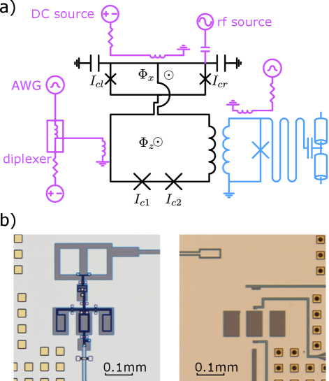
The measured CSFQ, together with the control and readout circuitry is schematically shown in Fig. 1(a). The CSFQ has a main loop and a secondary split-junction loop. In the two-state approximation, the CSFQ has the Hamiltonian
| (3) |
where is the reduced Planck’s constant, is the persistent current in the qubit main loop, is the tunneling amplitude between the two persistent current states, is the effective flux bias symmetry point, and are the qubit Pauli operators in the persistent current basis. The flux bias is the externally applied flux in the secondary loop. The flux bias is the effective flux bias in the main loop, defined such that the native crosstalk from the -loop is accounted for [25]. To a large extent controls the longitudinal field strength while controls the transverse field strength, hence the name and respectively. The -loop has a symmetrized design, allowing nearly independent control of the qubit’s transverse and longitudinal field (see Appendix B).
The external flux biases are controlled by currents through on-chip flux-bias lines, which are supplied by DC voltage sources and arbitrary waveform generators (AWGs) at room temperature, combined through cryogenic diplexers. In the experiment reported here, the high-frequency port of the diplexer that controls the -loop was unresponsive, and is hence neglected in the schematic in Fig. 1(a). In addition to flux biasing, the CSFQ is capacitively coupled to an rf source, allowing microwave excitation of the qubit.
Readout of the qubit is achieved by coupling the qubit -loop inductively to an rf-SQUID-terminated -resonator, coupled to a transmission line. The external flux bias of the rf-SQUID, is controlled by current through the on-chip bias line. When , the resonator is at its maximum frequency and the qubit-resonator coupling is linear. At this point, the resonator experiences a qubit-state-dependent dispersive shift. Away from zero bias, the resonator has a flux-sensitive resonance, which can be used for persistent current basis readout of the qubit (see Appendix C for more details regarding the qubit-resonator interaction).
The device is fabricated at MIT Lincoln Laboratory using a flip-chip process [62], combining a high-coherence qubit chip hosting the CSFQ, and a control chip that hosts the readout and control circuitry. Optical images of the two chips are shown in Fig. 1(b).
III Device characterization
In this section, we discuss the characterization measurements for the CSFQ. We note that details of the measurement setup and circuit modelling have been given in a related manuscript [63], and we focus the discussion here on aspects that concern annealing implementation with the CSFQ.
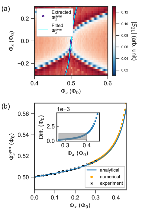
Experiments were performed with the device cooled down in a dilution refrigerator, with base temperature of about 10 mK. The crosstalk between the flux-bias lines was measured using the iterative procedure introduced in Ref. [64]. After three iterations, the error in flux biasing is expected to be about , with being the flux quantum. In Fig. 2 we show the transmission through the line coupled to the resonator, at a frequency near the resonator maximum frequency versus the calibrated external fluxes . This measurement shows that the symmetry point has a non-linear dependence on . This is due to the asymmetry between the two junctions in the DC-SQUID, which results in an effective contribution of the -loop flux to the -loop [65]. Assuming negligible -loop inductance, the -loop symmetry point is given by [39]
| (4) |
where is the junction asymmetry, with being the critical current of the left(right) junction in the DC-SQUID. The symmetry point can be extracted by checking the point of reflection symmetry for each trace of the transmission measurement at each value of , and the fitted asymmetry is . To verify the effect of finite -loop inductance, we use a full circuit model (see Appendix in Ref. [64]) to numerically extract the symmetry points and compare with the analytical expression. As shown in Fig. 2(b), using the same junction asymmetry , the discrepancy between the numerically simulated and analytical grows larger as increases, but always remain below for the range where the coherence measurements were performed, justifying the use of the analytical expression.
Once the crosstalk and junction asymmetry are calibrated, spectroscopy of the qubit is performed at a range of and biases, with the resonator SQUID biased at . A circuit model of the device is fit to the transition frequencies between ground, first and second excited states. The model includes the full capacitance matrix between islands, the loop inductances, and the Josephson junction critical currents, and is simulated using a package developed in Ref. [66] (see Appendix in Ref. [64] for circuit parameters).
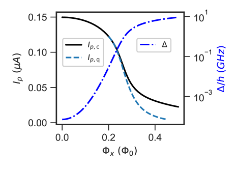
Using the circuit model, the qubit persistent current and tunneling amplitude versus the flux bias in the -loop can be obtained. The persistent current can be calculated using two different methods. In the first method, we rely on the operator matrix element defined on the CSFQ circuit
| (5) |
where is the circuit ground (excited) state, and is the circuit Hamiltonian, all evaluated at the symmetry point . In the second method, we find the ground-to-excited-states transition frequencies and fit to the qubit frequencies given by the two-state Hamiltonian Eq. 3. The corresponding persistent current is denoted as . In Fig. 3 we show versus . It can be seen that they agree with each other for small values of . At larger , becomes smaller than . This can be seen as a result of the breakdown of the two-state approximation, as the lowest energy states of the circuit are no longer spanned by the two persistent current states as (or equivalently the tunneling amplitude ) increases. This could lead to deviation from the transverse field Ising model typically used to describe a quantum annealer, though its impact is likely small for adiabatic evolution. Its impact in the case of non-adiabatic evolution will be studied in future work.
When compared with rf-SQUID flux qubits used in commercially available annealers, the CSFQ presented here has a persistent current that is at least an order of magnitude smaller, hence reducing its sensitivity to flux noise. The smaller also leads to a smaller interaction strength between qubits, which potentially limits the optimization problems that can be mapped to the annealer. We note that this could be compensated by galvanic coupling, using shared segments of loops [67], and even shared junction or junction arrays between the circuits that need to be coupled.
The simulated tunneling amplitude , also the qubit frequency at the symmetry point, is shown in Fig. 3. To implement a standard annealing experiment, the CSFQ is initialized at a large , around , and then the tunneling amplitude is gradually reduced following a specific annealing schedule. The CSFQ has a more gentle dependence of on as compared to the rf-SQUID qubit. Given the same resolution in the biasing sources, this dependence allows finer control of the annealing schedule, and assists in future experimental demonstrations of novel annealing protocols, such as those proposed in Ref. [68, 69].
IV Characterization of decoherence and discussion of results
In this section we present the measurements of the relaxation and dephasing times of the CSFQ. We note that coherence times are only well-defined when the system is weakly coupled to the environment, which is commonly the case in devices made for GMQC. In the context of annealing, the validity of the weak-coupling approximation depends on the relative strength of the qubit fields and the noise. In this work, we measure the coherence times for qubit frequency down to , below which thermally excited qubit population becomes significant. Although qubit state initialization at lower qubit frequencies is possible through high-fidelity single-shot readout [70], we do not pursue them in this work, as the available measurement range is enough to determine the strengths of the different noise, and for small enough , the weak-coupling limit eventually breaks down [63].
IV.1 Relaxation time measurements
We first discuss the relaxation data, which is shown in Fig. 4. The relaxation time was measured by initializing the qubit to the first excited state with a pulse and then performing readout after a variable delay time. The relaxation time is measured both as a function of , at the -loop symmetry point , as shown in Fig. 4(a), and as a function of near the symmetry point at three different , as shown in Fig. 4(c). At each , the relaxation measurement (and dephasing measurement presented later) at the symmetry point is repeated 30 times, and the average value is reported. We see that as varies from to , corresponding to changing from to , the at the -loop symmetry point increases at first, reaching a maximum at , and then decreases. This is similar to other coherence studies on flux qubits and fluxoniums [29, 39, 50], where the qubit coherence is limited by flux noise at lower frequency, and transitions to a different noise channel at frequencies higher than .
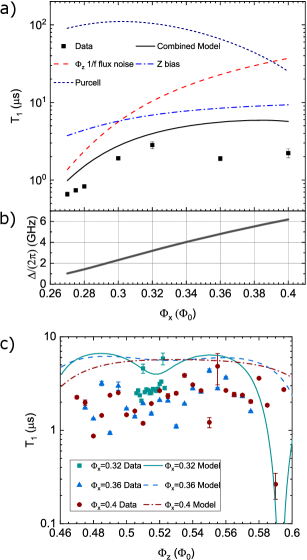
To better understand the relaxation data, we consider several relaxation channels and show their individual and combined calculated relaxation times in Fig. 4, including intrinsic flux noise in the -loop, thermal noise from the -loop bias line and Purcell effect due to the readout resonator. We assume the intrinsic flux noise has a noise PSD of , with being the angular frequency and the noise power at , set by fitting to the dephasing time (see Section IV.2). The flux-bias line can be modelled as a 50- impedance in parallel with a bias inductor that is coupled to the qubit loops. The noise temperature of the bias line can be estimated based on the attenuations used along the signal line [71]. The relaxation time due to Purcell effect is estimated by [72]
| (6) |
Here , , and are the resonator, qubit transition frequencies and the linear coupling strength between the qubit and the resonator. The coupling strength is calculated using the circuit model parameters (see Appendix C for the qubit-resonator interaction model and Appendix in Ref. [63] for the circuit parameter values), and is found to range from about to depending on the flux bias. The resonator decay rate is estimated based on resonator linewidth measurements. At the readout point, the resonator frequency and decay rate are and . Besides the above noise channels, we also note that the intrinsic flux noise in the -loop has negligible contribution to relaxation. The microwave port of the -bias line, if working, would lead to additional relaxation due to thermal noise on the -bias line. This is estimated to make substantial contribution to relaxation for , limiting to about . Details of the relaxation calculations are given in Appendix D. As shown in Fig. 4, at each -flux bias , the predicted relaxation time by combining the above known sources of noise comes within a factor of 2 of the highest measured at that value of .
We discuss the potential causes for the disagreement between the experimental data and the model used for energy relaxation. First, at lower , the noise power could differ from the noise power extrapolated using the dephasing time fits based on the simple dependence. Indeed, measurements done on devices fabricated using similar process show that the intrinsic flux noise has dependence, with [29, 40]. This means that the flux noise power at the qubit frequency is potentially higher than that assuming . Second, at higher , or qubit frequency, we note that there is significant scatter in the measured data, especially at values of . This can be seen from the versus measurements shown in Fig. 4(c). The scatter in the data could be due to coupling to microscopic two-level systems (TLS). Although the underlying physical nature of TLSs are still under active investigation [61], resonant coupling to TLSs usually leads to variations in over qubit frequencies [73], and sometimes fluctuations over time [74]. This is also in line with recent measurement on fluxoniums, showing that TLSs indeed have a strong contribution to relaxation at high frequencies [50]. Besides TLSs, quasi-particles are known to cause fluctuations in [75] over time. To check the effect of quasi-particles, we compared fits using a simple exponential decay model and a model incorporating non-exponential decay due to quasi-particle tunneling during the measurement. The reduced chi-squared of the fits are almost the same in the two models, and therefore quasi-particle is likely not a dominant source of loss in our experiment.
Previous coherence measurement on flux qubits show that at higher qubit frequency is likely limited by intrinsic flux noise with an ohmic or superohmic noise spectrum [39, 50], although it could be difficult to distinguish ohmic flux noise to charge noise [29]. We found that including ohmic flux or charge noise in the model does not lead to substantially better agreement between the simulation and the measurement. This suggests that at higher qubit frequencies, thermal noise from the bias line is likely the main source of relaxation, along with TLSs which caused additional scatter. The large bias line noise is due to the use of a large bandwidth low-pass filter at 12 GHz, opted to explore fast annealing and allow spectroscopic characterization through the bias lines. This could be mitigated by reducing the cutoff frequency to values of the order of 1 GHz, which retains the compatibility for most annealing protocols, while suppressing bias line induced relaxation rate to below the intrinsic flux noise limit.
IV.2 Dephasing time measurements
We next discuss the dephasing measurement, which is also performed at a range of and flux biases. times were measured using a Ramsey protocol (see for example Ref. [21]) which consists of initializing the qubit with a /2 pulse (detuned approximately 10 MHz from the qubit transition frequency) and then applying a second pulse after a variable delay time just before performing readout. As shown in Fig. 5(a), at the bias symmetry point, the Ramsey pure dephasing time varies from to as is reduced from to . The spin-echo dephasing time , measured with a sequence that has an additional pulse in between the two pulses [21], shows an improvement of about a factor of . This improvement, and the fact that all the measured coherence decays have been well-fitted with an Gaussian envelope, are consistent with dephasing dominated by noise. When examining the dependence of , it is found that the maximum dephasing time occurs near, but to the left of the bias symmetry point , which stands in contrast to the non-tunable flux qubit.
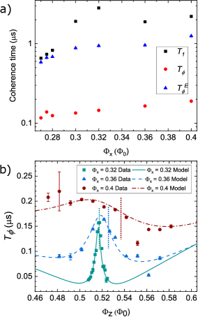
To model dephasing, we assume flux noise in the - and -loops are the only sources of dephasing, with noise power spectral density and respectively. In addition, we assume the flux noise in the - and -loops have correlated noise PSD , represented by the dimensionless coefficient, . The frequency sensitivity to flux noise is determined directly from the circuit model, without the two-state approximation. The noise powers that fit the measured best are , . These numbers are consistent with previous devices fabricated using a similar process [67], considering that flux noise power scales as length over width of the loop wires [37, 40].
The best fit of the dephasing times indicates a correlation coefficient of (see Appendix E.2). Flux noise correlation in tunable flux qubits have been measured previously [76, 50], and it has been pointed out that positive (negative) correlation shifts the maximum dephasing time to the left (right) of the symmetry point. Assuming flux noise arises from uniformly distributed environmental spins on the metal surface of the superconducting loop, Ref. [76] shows that the correlation could be understood in terms of spins that occupy the shared arm between the - and -loops. However, given the symmetrized -loop design used here, the expected correlation using this simple model for flux noise is zero, and hence does not explain the measured correlation.
Junction asymmetry could also lead to an offset between the maximum dephasing time and the qubit symmetry point. To see this, one could define another effective -flux bias , such that the symmetry point in is independent of . This means
| (7) |
where is given by Eq. 4 when the -loop inductance is negligible. Then it can be shown that the noise correlation coefficient between and is given by (see Appendix B)
| (8) |
Therefore, for negligible , as would be the case if noise purely comes from uniformly distributed spins on the metal surface, would be negative given a positive junction asymmetry . In other words, the effect of junction asymmetry in the device is to shift the point of maximum dephasing time to the right of the symmetry point, which is the opposite of what is observed experimentally. We note that this apparent offset should not be confused with the fitted correlation , as the fitting uses numerically extracted frequency sensitivity to and , which implicitly contains information about the asymmetry.
To further investigate the source of this correlation, we considered additional sources of dephasing, including bias line thermal noise, voltage noise of the bias source, photon shot noise, second-order coupling to flux noise, charge noise and junction critical-current noise (see Appendix E.4). We find that using previously reported values of noise of the critical current of the junctions, its contribution to dephasing can be non-negligible compared to dephasing due to first-order coupling to flux noise. Furthermore, junction critical-current noise leads to maximum dephasing time to the left of , hence could contribute to the apparent positive correlation between the two flux biases. In addition, we note that in contrast to previous studies, where the flux noise correlation could mostly be explained by environmental spins local to the metal surface of the superconducting loop [76, 50], our device has a flip-chip architecture, involving a ground plane on the interposer chip facing the loops (see Figure. 1). This points to the possibility of screening effect and environmental spins on the interposer ground plane as a source of noise correlation, which will be studied in future work.
We also observed over multiple cooldowns of the dilution fridge and changes to the setup that the choice of bias source could have an impact on the coherence times as well. Experiments performed during earlier cooldowns used AWGs as the DC bias sources for the device. After switching from using AWGs to a lower noise DC bias source for the -bias, we found the measured Ramsey pure dephasing time at improved from ns initially to ns after the switch. In Appendix E.3, we show that by assuming the AWG has a combined and white noise spectrum at low frequency, it alone could lead to dephasing time of ns. This is roughly consistent with the reduction in Ramsey dephasing time when the AWG is used, given the crude model of the AWG noise. As the DC bias source does not support fast annealing, strategies need to be developed to mitigate the noise from the AWG. This could be done by either using a cryogenic bias-T to combine the DC and fast signal, allowing smaller coupling strength of the more noisy signal, or applying heavier filtering to the fast signal and correct for distortions in-situ [77].
V Noise in annealing parameters
It is useful to put the noise measured here in the context of annealing applications. For a “single-qubit anneal” [65, 78], the qubit Hamiltonian starts with a large value of , at which the qubit is initialized in the ground state, and the qubit Hamiltonian is gradually changed to a target Hamiltonian where is close to zero. The only parameter defining the target Hamiltonian is the qubit longitudinal field
| (9) |
Noise in the control fluxes gives rise to noise in the annealing parameters , with the same frequency dependence. We focus on the intrinsic flux noise, assuming noise arising from wiring and electronics can be minimized through careful engineering. Using the two-state approximation Hamiltonian Eq. 3, we find the individual and correlated noise in to be
| (10) | ||||
| (11) | ||||
| (12) |
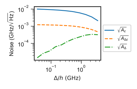
where is the power of the flux noise correlation. In Fig. 6 we show these three quantities versus the transverse field , for the target longitudinal field , noting these quantities are weakly dependent on . It can be seen that the noise, is always the dominant noise factor. The correlated noise is mainly due to the measured flux noise correlation, and is about an order of magnitude lower than . The noise in is comparable to for large , but diminishes quickly with decreasing . The role of the relative strength of the noises will be explored in future work. One interesting direction is to extend the previous analysis of the effect of correlated noise on single qubit Landau-Zener tunneling [79], to the general case of multi-qubit annealing.
VI Conclusion
We have presented a detailed characterization of coherence in a CSFQ design relevant for quantum annealing. We measured the relaxation and dephasing times and modelled them considering all relevant noise sources. We find that the values are influenced primarily by flux noise with additional contributions from bias line thermal noise and TLSs at higher frequencies. The measured dephasing time is dominated by flux noise, with a possible contribution from noise in the junction critical current. We point out that for annealing applications, the external flux biases can introduce significant relaxation and dephasing as compared to the intrinsic noise of the qubit. This suggests that future annealing experiments that aim to combine high-coherence and high control flexibility need to carefully evaluate the trade-off between the added noise and the improved control bandwidth.
Additionally, we observe a positive correlation between the and flux noise, as manifested in the maximum dephasing time versus occurring to the left of the bias symmetry point. This correlation may arise due to environmental spins on the interposer ground plane, and junction critical-current noise. Future experiments that are able to distinguish the different sources of noise are needed to quantitatively determine the origin of this noise correlation.
Our work provides a detailed characterization of noise sources of a flux qubit, relevant for future analysis of coherent annealers based on CSFQs. Besides quantum annealing, the work presented here is also relevant for flux qubit devices made for GMQC, such as fluxonium qubits. Future work will be directed at extending the coherence characterization to the strong coupling limit and multi-qubit systems, as well as studying coherence in a dynamic setting, which will lead to a deeper understanding of the role of coherence in quantum annealing.
Acknowledgements.
We thank the members of the Quantum Enhanced Optimization (QEO)/Quantum Annealing Feasibility Study (QAFS) collaboration for various contributions that impacted this research. In particular, we A. J. Kerman for guidance on circuit simulations, S. Novikov for assisting the chip design, and K. Zick for coordinating the experimental efforts in the collaboration. We gratefully acknowledge the MIT Lincoln Laboratory design, fabrication, packaging, and testing personnel for valuable technical assistance. The research is based upon work supported by the Office of the Director of National Intelligence (ODNI), Intelligence Advanced Research Projects Activity (IARPA) and the Defense Advanced Research Projects Agency (DARPA), via the U.S. Army Research Office contract W911NF-17-C-0050. The views and conclusions contained herein are those of the authors and should not be interpreted as necessarily representing the official policies or endorsements, either expressed or implied, of the ODNI, IARPA, DARPA, or the U.S. Government. The U.S. Government is authorized to reproduce and distribute reprints for Governmental purposes notwithstanding any copyright annotation thereon.Appendix A Noise power spectral density and correlation
In this work, we define the noise power spectral density (PSD) of a random variable as the Fourier transform of its autocorrelation function,
| (13) |
If the noise arises from a quantum bath, the noise PSD is asymmetric in positive and negative frequencies. However, our noise measurement is only sensitive to the symmetrized noise spectrum, which we define as
| (14) | ||||
| (15) |
The symmetrized correlation between two random variables and is given by the cross power spectral density
| (16) | ||||
| (17) |
where is a dimensionless number describing the relative correlation between the two noise variables.
Appendix B Definition of effective fluxes and noise correlations
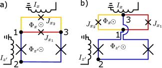
Figure 7 shows the circuit schematic for a tunable CSFQ, including the flux-bias lines, using a planar and a symmetrized -loop geometry. In both cases the flux biases are applied through the loops labeled and . These loops are defined as follows:
| (18) | |||
| (19) |
where the numbers are the node indices, as indicated in Fig. 7. The external fluxes in these two loops are denoted by respectively.
We also introduce
| (20) |
In the experiments and simulations we use the coordinates. When the junctions of the -loop are symmetric, the potential energy of the flux qubit is a symmetric double well when , with a barrier that is controlled by . The symmetrized -loop design allows tuning of the tunneling with the bias current , while remaining near the qubit symmetry point without changing , which is advantageous for annealing.
An asymmetry between the critical currents of the -loop junctions shifts the symmetry point that corresponds to a symmetric double well. Since we are interested in the shift in flux bias corresponding to a maximum coherence, relative to the symmetry point, it is also useful to define , a coordinate in which the symmetry point is independent of . This is
| (21) |
where is the induced shift due to -loop junction asymmetry.
Next we relate the flux noise PSDs and correlations among the three different -flux bias conventions, which further clarifies the role of loop geometry and junction asymmetry on the measured flux noise correlation. To make a connection between noise in and , we consider small variations in the flux biases,
| (22) |
This allows us to calculate the PSD of
| (23) |
To obtain the cross PSD between and use
| (24) |
which gives
| (25) | ||||
| (26) |
where is the dimensionless correlation between and flux noise. Similarly, the noise in can be related to noise in by considering the relation
| (27) |
which gives
| (28) |
For the cross PSD between and we use
| (29) |
which gives
| (30) |
Previous studies [76, 80] suggest that flux noise can be explained by local fluctuating spins uniformly distributed along the surface of the circumference of the qubit loops. This model indicates the scaling of flux noise power with the geometry of superconducting loops as
| (31) |
Here refers to the flux noise power from a particular superconducting loop or arm, is a parameter assumed to be constant for the same fabrication procedure, and are the length and width of a superconducting loop or arm. Assuming independent contribution to flux noise from the spins on each segment of the superconducting loop, We can relate the fluctuations to the fluctuation on each segment,
| (32) | ||||
| (33) |
Then
| (34) |
We can also obtain in terms of the contribution from the two arms since
| (35) |
Given the red and yellow arms are of equal length and wire width by design in the device measured in this work, then
| (36) | ||||
| (37) | ||||
| (38) |
where in the second line we used Eq. 34 and Eq. 35. To summarize the results obtained by assuming the geometric dependence of intrinsic flux noise and a symmetric -loop, we have
| (39) | |||
| (40) | |||
| (41) |
Combining these with Eq. 23 and 25 we get
| (42) | ||||
| (43) |
Therefore for the symmetrized -loop design, the expected flux noise correlation coefficient is zero.
Appendix C Modelling rf-SQUID-terminated resonator
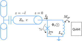
The schematic of the readout resonator is shown in Fig. 8, which consists of an rf-SQUID-terminated resonator, coupled to the qubit via a mutual inductance between the rf-SQUID and the qubit -loop. To calculate various properties of the resonator coupled to the qubit, such as dispersive shift and Purcell loss, a quantum mechanical description of the resonator is required. This can be derived by first considering the energy stored in the resonator,
| (44) |
where are voltage and currents along the resonator waveguide, is the length of the waveguide, are the waveguide characteristic impedance and speed of light. The SQUID can be modelled as an effective inductance , which can be found by minimizing the classical potential of an rf-SQUID [81]. The above expression for the resonator energy can be converted into quadratic form, allowing canonical quantization of the resonator [82]. This leads to an expression for the quantum bias current going into the SQUID, in terms of the harmonic oscillator operators
| (45) | ||||
| (46) |
with being the resonance frequency.
Since in our design, the qubit is coupled inductively to the geometric inductance of the rf-SQUID, we need to further relate the SQUID bias current to the current flowing through the SQUID geometric inductance. Assuming small values of , which is justified when the energy in the resonator is low, the current through the geometric inductance is
| (47) | ||||
| (48) |
where in the second line we performed a Taylor expansion of around . The coefficients of the Taylor expansion can be found numerically by minimizing the SQUID potential at a range of . The term corresponds to screening current in the SQUID and effectively shifts the qubit bias. The coefficients , are SQUID bias dependent and give rise to linear and non-linear interactions between the resonator and the qubit. Finally the interaction Hamiltonian between the resonator and the qubit is
| (49) |
where is the mutual inductance between the qubit and the SQUID geometric inductance, and is the qubit operator participating in the interaction.
Appendix D Relaxation
We consider the qubit relaxation time in general to be given by
| (50) | ||||
| (51) |
where is the Purcell effect decay rate to the resonator, are the relaxation times due to the intrinsic flux noise in the loops, are the relaxation times due to Johnson-Nyquist noise in the bias lines, and are additional ohmic noises that couple to the qubit charge(flux) degrees of freedom [83, 29, 39].
The relaxation time due to Purcell loss is estimated by [72]
| (52) |
where is the exchange interaction strength between the qubit and the resonator, is the resonator frequency and is the resonator decay rate.
For the rest of the noise channels, we assume the noise is weak and the decay rate from the Bloch-Redfield theory (or equivalently Fermi’s Golden rule) is given by [21],
| (53) |
where is understood as the qubit operator that is coupled to the noise, and is the noise PSD of at qubit frequency . For the intrinsic flux noise, we assume they are of the form , with the same noise amplitude as found in the pure dephasing rate fits. For the Johnson-Nyquist noise, we consider the bias line as an inductor with inductance shunted by an impedance of . The current noise is given by
| (54) | ||||
| where | (55) |
and based on electromagnetic simulation. To compute the noise temperature , we assume that each attenuator along the signal delivery chain acts as a beam-splitter [71], so that the thermal noise photon number at stage is given as
| (56) |
where and are the temperature of the fridge plate and the corresponding attenuation attached to that plate. The Bose-Einstein photon occupation number is given by . In particular for the -bias, we used , , dB attenuations at the , and stages of the dilution fridge. This attenuation scheme leads to an effective noise temperature of at , which is relatively high compared to the base temperature of the fridge.
The additional ohmic noise can be given as
| (57) |
with and the different noise coefficients corresponding to charge noise, flux noise and flux noise. Previous experiments on flux qubits have found that the dominant relaxation channel at higher qubit frequencies () could be either ohmic charge or (super)ohmic flux noise [29, 39, 50]. In our experiments, we found that including the ohmic flux and charge noise do not substantially improve the agreement between the model and the simulation, due to the relatively significant scatter in our data.
Appendix E Pure dephasing
Dephasing is caused by low-frequency fluctuations in the qubit energy splitting due to various noise sources. The noise spectrum of the qubit transition frequency is given by
| (58) |
where the summation runs over the noise sources under consideration. For classical noise, dephasing can be described by the decay [84], where is given by
| (59) |
Here is the filter function for the specific coherence measurement, and is a low-frequency cutoff determined by the total experiment time. We have for Ramsey and for spin-echo measurement. Their respective filter functions are
| (60) | ||||
| (61) |
In general the decay of is not exponential. We associate the pure dephasing time as the decay time, where .
E.1 Noises that couple via the fluxes
In order to realize the large energy scale required for annealing, the tunable CSFQs have relatively large superconducting loops and flux sensitivities. This large sensitivity, together with the measured flux noise correlation, motivate grouping the noises that couple to control fluxes together. We consider three different such sources, intrinsic flux noise, Johnson-Nyquist noise of the bias lines and noise due to biasing sources. Denoting the intrinsic flux noise on the two fluxes as , the Johnson-Nyquist current noise on the two bias lines as and the voltage noise from the bias sources as , the self and cross PSD of the two flux biases are
| (62) | ||||
| (63) | ||||
| (64) | ||||
| (65) |
where are the mutuals between the bias lines and the fluxes, and are the resistances between the source and the bias line on the chip. We note that the intrinsic flux noise is non-negligible at both low and high frequencies. The voltage noise from the bias sources is only strong at low frequencies, as the bias source is coupled to the device through a low-pass filter, and the Johnson-Nyquist current noise is only apparent at high frequencies.
E.2 Dephasing due to intrinsic flux noise alone
The intrinsic flux noise usually has a noise PSD of the form
| (66) |
for , where . If dephasing is dominated by flux noise, we can assume has the same frequency dependence, with
| (67) |
In this case, the integral in Eq. (59) can be simplified, which leads to a dephasing time of
| (68) |
Following Ref. [67], for Ramsey and spin-echo measurements, the factors can be determined numerically by
| (69) | ||||
| (70) |
where is the typical free evolution time in a single Ramsey sequence.
To fit the measured Ramsey dephasing times, Eqn. 68 is applied. The noise power is related to the flux noise powers via
| (71) | ||||
| (72) |
with extracted numerically from the circuit model. The factor is found by using and , and the noise exponent is assumed to be .
E.3 Dephasing due to biasing sources
During a separate cooldown of the device, a different measurement setup was used and the coherence time of the device dropped significantly. Among other changes in the setup, we found that biasing the qubit circuit using an AWG is the likely cause of the lower coherence. In this section, we present the estimated dephasing rate due to typical noise from the AWG (Keysight model M3202a).
The AWG can be considered to have a classical voltage noise source, with a noise PSD that is close to a combination of and white noise. For low-frequency biasing, the noise is also low-pass filtered at some cutoff frequency . This motivates a simple voltage noise PSD for the AWG, given by
| (73) |
where is related to the noise power of the part, describes the white noise power and we assumed the filter is first-order for simplicity.
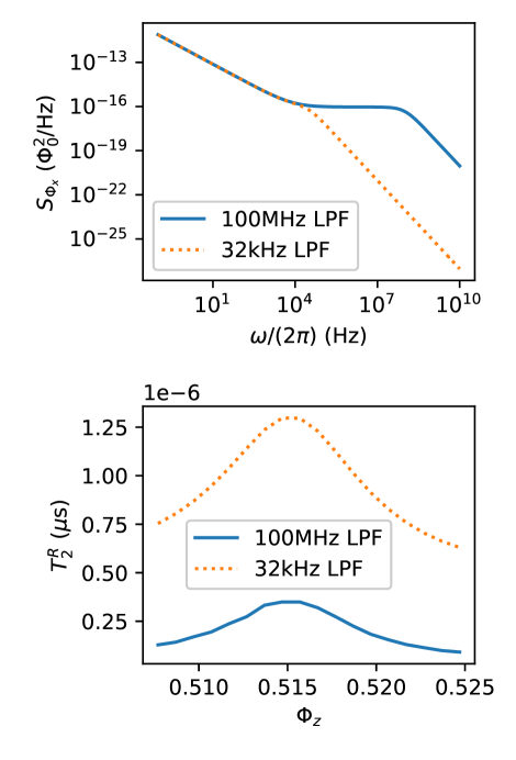
For the numerical computation, we take and , for both the and low-frequency bias. Ignoring other sources of noise, we show the estimated flux bias noise PSD for two different low-frequency cutoffs, kHz and MHz in Fig. 9. The dephasing rate is computed numerically for a range of at , by solving from Eq. 59, which is shown in Fig. 9(b). It can be seen that when the low-frequency cutoff is MHz, the dephasing rate becomes close to the intrinsic flux noise limited rate shown in the main text. When the low-frequency cutoff is kHz, the dephasing rate due to voltage noise is about an order of magnitude larger.
For the data presented in the main text, the DC bias has a low-frequency cutoff of kHz, and the biasing source is a Yokogawa DC voltage source (model GS200), which is expected to have lower noise than the AWG. Furthermore, the microwave port of -bias couples about 20 times more weakly than the DC port. The microwave port of -bias is unused. These considerations allow us to eliminate the effect of the biasing sources on the dephasing.
E.4 Estimated dephasing for other noise sources
In this section, we consider a number of additional sources of dephasing.
Defects in the junction tunneling barrier could lead to noise of the critical current of the junctions [51] and have been shown to be the main source of dephasing at the symmetry point in some earlier flux qubits [52]. To estimate the critical-current noise induced dephasing, we follow Ref. [52] and assume a normalized critical-current noise of on each of the four junctions independently. The noise sensitivity to the ’th junction’s critical current can be computed numerically from the circuit model, and leads to a noise sensitivity to the normalized critical-current noise defined as
| (74) |
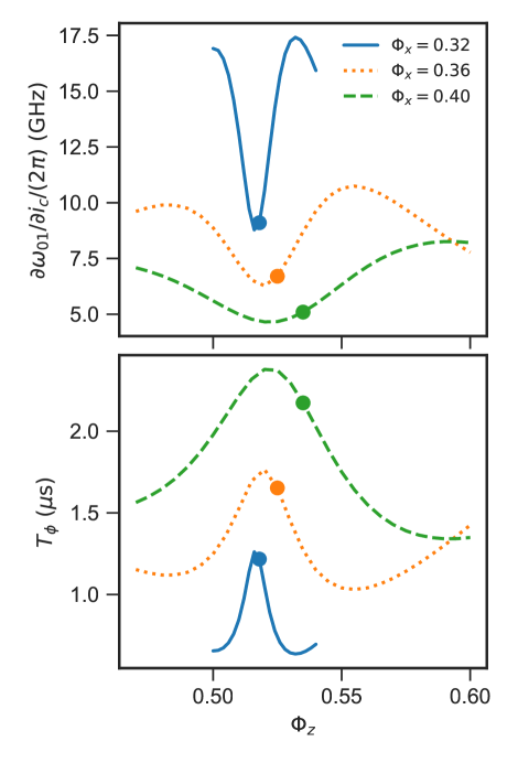
where is junction critical current normalized by its nominal value . In Fig. 10 we show the critical-current noise sensitivity and the corresponding dephasing time over different biases. We see that the dephasing rate can be a substantial fraction of the measured dephasing rate. We also note that for each , the bias corresponding to the minimum sensitivity, and hence maximum dephasing time, is to the left of the symmetry point. This trend is in line with the experimentally measured Ramsey dephasing versus . Therefore the critical-current noise could be a potential explanation for the apparent correlation between the - and -loop flux noise, although further understanding and investigations into the physical origin of these noises are required to distinguish them.
It was previously observed in high-coherence CSFQs that the dominant noise channel at the symmetry point is photon-shot noise [29], with dephasing rate given by
| (75) |
where is the resonator decay rate and is the qubit-induced dispersive shift of the resonator, and is the average thermal photon in the resonator. In our experiments, at , we found a dispersive shift of , and a resonator decay rate of . To obtain a dephasing rate of , the required average thermal photon number is , much higher than the expected value, given the readout resonator should be reasonably well thermalized with the readout line in the fridge. Therefore photon-shot noise is unlikely to be dominant in our device.
We also consider the second-order coupling of flux noise following [21]. Given our typical experimental timescales, we take the quasistatic limit of flux noise and find that the second-order coupling to flux noise contributes to dephasing rate
| (76) |
Using the numerically simulated qubit spectrum and the fitted flux noise amplitudes, we estimate that the second-order coupling to flux noise leads to , which is negligible compared to the dephasing due to first-order coupling.
It has also been reported that quasi-particles could lead to frequency fluctuations in certain flux qubits [85]. We checked the variation in in our circuit as a function of charge offsets in each island, and found a maximum of kHz, which is much smaller than the observed . Therefore dephasing due to quasi-particles or charge noise are likely negligible.
Finally, we briefly note that the thermal noise of the bias lines at low frequency leads to a dephasing time of about and can be neglected.
References
- Kadowaki and Nishimori [1998] T. Kadowaki and H. Nishimori, Quantum annealing in the transverse Ising model, Phys. Rev. E 58, 5355 (1998).
- Farhi et al. [2001] E. Farhi, J. Goldstone, S. Gutmann, J. Lapan, A. Lundgren, and D. Preda, A Quantum Adiabatic Evolution Algorithm Applied to Random Instances of an NP-Complete Problem, Science 292, 472 (2001).
- Hauke et al. [2020] P. Hauke, H. G. Katzgraber, W. Lechner, H. Nishimori, and W. D. Oliver, Perspectives of quantum annealing: Methods and implementations, Rep. Prog. Phys. 83, 054401 (2020).
- Amin et al. [2018] M. H. Amin, E. Andriyash, J. Rolfe, B. Kulchytskyy, and R. Melko, Quantum Boltzmann Machine, Phys. Rev. X 8, 021050 (2018).
- King et al. [2021] A. D. King, J. Raymond, T. Lanting, S. V. Isakov, M. Mohseni, G. Poulin-Lamarre, S. Ejtemaee, W. Bernoudy, I. Ozfidan, A. Y. Smirnov, M. Reis, F. Altomare, M. Babcock, C. Baron, A. J. Berkley, K. Boothby, P. I. Bunyk, H. Christiani, C. Enderud, B. Evert, R. Harris, E. Hoskinson, S. Huang, K. Jooya, A. Khodabandelou, N. Ladizinsky, R. Li, P. A. Lott, A. J. R. MacDonald, D. Marsden, G. Marsden, T. Medina, R. Molavi, R. Neufeld, M. Norouzpour, T. Oh, I. Pavlov, I. Perminov, T. Prescott, C. Rich, Y. Sato, B. Sheldan, G. Sterling, L. J. Swenson, N. Tsai, M. H. Volkmann, J. D. Whittaker, W. Wilkinson, J. Yao, H. Neven, J. P. Hilton, E. Ladizinsky, M. W. Johnson, and M. H. Amin, Scaling advantage over path-integral Monte Carlo in quantum simulation of geometrically frustrated magnets, Nat. Comm 12, 1113 (2021).
- Albash and Lidar [2018] T. Albash and D. A. Lidar, Adiabatic quantum computation, Rev. Mod. Phys. 90, 015002 (2018).
- Mizel et al. [2007] A. Mizel, D. A. Lidar, and M. Mitchell, Simple Proof of Equivalence between Adiabatic Quantum Computation and the Circuit Model, Phys. Rev. Lett. 99, 070502 (2007).
- Aharonov et al. [2008] D. Aharonov, W. van Dam, J. Kempe, Z. Landau, S. Lloyd, and O. Regev, Adiabatic Quantum Computation Is Equivalent to Standard Quantum Computation, SIAM Rev. 50, 755 (2008).
- Kjaergaard et al. [2020] M. Kjaergaard, M. E. Schwartz, J. Braumüller, P. Krantz, J. I.-J. Wang, S. Gustavsson, and W. D. Oliver, Superconducting Qubits: Current State of Play, Annu. Rev. Condens. Matter Phys. 11, 369 (2020).
- Blais et al. [2021] A. Blais, A. L. Grimsmo, S. M. Girvin, and A. Wallraff, Circuit quantum electrodynamics, Rev. Mod. Phys. 93, 025005 (2021).
- Harris et al. [2010] R. Harris, J. Johansson, A. J. Berkley, M. W. Johnson, T. Lanting, S. Han, P. Bunyk, E. Ladizinsky, T. Oh, I. Perminov, E. Tolkacheva, S. Uchaikin, E. M. Chapple, C. Enderud, C. Rich, M. Thom, J. Wang, B. Wilson, and G. Rose, Experimental demonstration of a robust and scalable flux qubit, Phys. Rev. B 81, 134510 (2010).
- Quintana [2017] C. M. Quintana, Superconducting Flux Qubits for High-Connectivity Quantum Annealing without Lossy Dielectrics, Ph.D. thesis, UC Santa Barbara (2017).
- Novikov et al. [2018] S. Novikov, R. Hinkey, S. Disseler, J. I. Basham, T. Albash, A. Risinger, D. Ferguson, D. A. Lidar, and K. M. Zick, Exploring More-Coherent Quantum Annealing, in 2018 IEEE International Conference on Rebooting Computing (ICRC) (2018) pp. 1–7.
- Johnson et al. [2011] M. W. Johnson, M. H. S. Amin, S. Gildert, T. Lanting, F. Hamze, N. Dickson, R. Harris, A. J. Berkley, J. Johansson, P. Bunyk, E. M. Chapple, C. Enderud, J. P. Hilton, K. Karimi, E. Ladizinsky, N. Ladizinsky, T. Oh, I. Perminov, C. Rich, M. C. Thom, E. Tolkacheva, C. J. S. Truncik, S. Uchaikin, J. Wang, B. Wilson, and G. Rose, Quantum annealing with manufactured spins, Nature 473, 194 (2011).
- [15] QPU-Specific Characteristics—D-Wave System Documentation.
- King et al. [2022a] A. D. King, J. Raymond, T. Lanting, R. Harris, A. Zucca, F. Altomare, A. J. Berkley, K. Boothby, S. Ejtemaee, C. Enderud, E. Hoskinson, S. Huang, E. Ladizinsky, A. J. R. MacDonald, G. Marsden, R. Molavi, T. Oh, G. Poulin-Lamarre, M. Reis, C. Rich, Y. Sato, N. Tsai, M. Volkmann, J. D. Whittaker, J. Yao, A. W. Sandvik, and M. H. Amin, Quantum critical dynamics in a 5000-qubit programmable spin glass (2022a), arXiv:2207.13800 [cond-mat, physics:quant-ph] .
- Siddiqi [2021] I. Siddiqi, Engineering high-coherence superconducting qubits, Nat. Rev. Mater. 6, 875 (2021).
- Amin et al. [2009] M. H. S. Amin, C. J. S. Truncik, and D. V. Averin, Role of single-qubit decoherence time in adiabatic quantum computation, Phys. Rev. A 80, 022303 (2009), 00043.
- Bloch [1957] F. Bloch, Generalized Theory of Relaxation, Phys. Rev. 105, 1206 (1957).
- Redfield [1957] A. G. Redfield, On the Theory of Relaxation Processes, IBM J. Res. Dev. 1, 19 (1957).
- Ithier et al. [2005] G. Ithier, E. Collin, P. Joyez, P. J. Meeson, D. Vion, D. Esteve, F. Chiarello, A. Shnirman, Y. Makhlin, J. Schriefl, and G. Schön, Decoherence in a superconducting quantum bit circuit, Phys. Rev. B 72, 134519 (2005).
- Leggett et al. [1987] A. J. Leggett, S. Chakravarty, A. T. Dorsey, M. P. A. Fisher, A. Garg, and W. Zwerger, Dynamics of the dissipative two-state system, Rev. Mod. Phys. 59, 1 (1987).
- Friedman et al. [2000] J. R. Friedman, V. Patel, W. Chen, S. K. Tolpygo, and J. E. Lukens, Quantum superposition of distinct macroscopic states, Nature 406, 43 (2000).
- Mooij et al. [1999] J. E. Mooij, T. P. Orlando, L. Levitov, L. Tian, C. H. van der Wal, and S. Lloyd, Josephson Persistent-Current Qubit, Science 285, 1036 (1999).
- Orlando et al. [1999] T. P. Orlando, J. E. Mooij, L. Tian, C. H. van der Wal, L. S. Levitov, S. Lloyd, and J. J. Mazo, Superconducting persistent-current qubit, Phys. Rev. B 60, 15398 (1999).
- Van Der Wal et al. [2000] C. H. Van Der Wal, A. C. J. Ter Haar, F. K. Wilhelm, R. N. Schouten, CJPM. Harmans, T. P. Orlando, S. Lloyd, and J. E. Mooij, Quantum superposition of macroscopic persistent-current states, Science 290, 773 (2000).
- You et al. [2007] J. Q. You, X. Hu, S. Ashhab, and F. Nori, Low-decoherence flux qubit, Phys. Rev. B 75, 140515 (2007).
- Steffen et al. [2010] M. Steffen, S. Kumar, D. P. DiVincenzo, J. R. Rozen, G. A. Keefe, M. B. Rothwell, and M. B. Ketchen, High-Coherence Hybrid Superconducting Qubit, Phys. Rev. Lett. 105, 100502 (2010).
- Yan et al. [2016] F. Yan, S. Gustavsson, A. Kamal, J. Birenbaum, A. P. Sears, D. Hover, T. J. Gudmundsen, D. Rosenberg, G. Samach, S. Weber, J. L. Yoder, T. P. Orlando, J. Clarke, A. J. Kerman, and W. D. Oliver, The flux qubit revisited to enhance coherence and reproducibility, Nat. Comm. 7, 10.1038/ncomms12964 (2016).
- Yurtalan et al. [2021] M. Yurtalan, J. Shi, G. Flatt, and A. Lupascu, Characterization of Multilevel Dynamics and Decoherence in a High-Anharmonicity Capacitively Shunted Flux Circuit, Phys. Rev. Appl. 16, 054051 (2021).
- Manucharyan et al. [2009] V. E. Manucharyan, J. Koch, L. I. Glazman, and M. H. Devoret, Fluxonium: Single Cooper-Pair Circuit Free of Charge Offsets, Science 326, 113 (2009).
- Nguyen et al. [2019] L. B. Nguyen, Y.-H. Lin, A. Somoroff, R. Mencia, N. Grabon, and V. E. Manucharyan, High-Coherence Fluxonium Qubit, Phys. Rev. X 9, 041041 (2019).
- Somoroff et al. [2021] A. Somoroff, Q. Ficheux, R. A. Mencia, H. Xiong, R. V. Kuzmin, and V. E. Manucharyan, Millisecond coherence in a superconducting qubit (2021), arXiv:2103.08578 [cond-mat, physics:quant-ph] .
- Yoshihara et al. [2006] F. Yoshihara, K. Harrabi, A. O. Niskanen, Y. Nakamura, and J. S. Tsai, Decoherence of Flux Qubits due to $1/f$ Flux Noise, Phys. Rev. Lett. 97, 167001 (2006).
- Kakuyanagi et al. [2007] K. Kakuyanagi, T. Meno, S. Saito, H. Nakano, K. Semba, H. Takayanagi, F. Deppe, and A. Shnirman, Dephasing of a Superconducting Flux Qubit, Physical Review Letters 98, 047004 (2007).
- Bialczak et al. [2007] R. C. Bialczak, R. McDermott, M. Ansmann, M. Hofheinz, N. Katz, E. Lucero, M. Neeley, A. D. O’Connell, H. Wang, A. N. Cleland, and J. M. Martinis, $1/f$ Flux Noise in Josephson Phase Qubits, Physical Review Letters 99, 187006 (2007).
- Lanting et al. [2009] T. Lanting, A. J. Berkley, B. Bumble, P. Bunyk, A. Fung, J. Johansson, A. Kaul, A. Kleinsasser, E. Ladizinsky, F. Maibaum, R. Harris, M. W. Johnson, E. Tolkacheva, and M. H. S. Amin, Geometrical dependence of the low-frequency noise in superconducting flux qubits, Phys. Rev. B 79, 060509 (2009).
- Yoshihara et al. [2014] F. Yoshihara, Y. Nakamura, F. Yan, S. Gustavsson, J. Bylander, W. D. Oliver, and J.-S. Tsai, Flux qubit noise spectroscopy using Rabi oscillations under strong driving conditions, Physical Review B 89, 020503 (2014).
- Quintana et al. [2017] C. M. Quintana, Y. Chen, D. Sank, A. G. Petukhov, T. C. White, D. Kafri, B. Chiaro, A. Megrant, R. Barends, B. Campbell, Z. Chen, A. Dunsworth, A. G. Fowler, R. Graff, E. Jeffrey, J. Kelly, E. Lucero, J. Y. Mutus, M. Neeley, C. Neill, P. J. J. O’Malley, P. Roushan, A. Shabani, V. N. Smelyanskiy, A. Vainsencher, J. Wenner, H. Neven, and J. M. Martinis, Observation of Classical-Quantum Crossover of 1/ Flux Noise and Its Paramagnetic Temperature Dependence, Phys. Rev. Lett. 118, 057702 (2017).
- Braumüller et al. [2020] J. Braumüller, L. Ding, A. P. Vepsäläinen, Y. Sung, M. Kjaergaard, T. Menke, R. Winik, D. Kim, B. M. Niedzielski, A. Melville, J. L. Yoder, C. F. Hirjibehedin, T. P. Orlando, S. Gustavsson, and W. D. Oliver, Characterizing and Optimizing Qubit Coherence Based on SQUID Geometry, Phys. Rev. Appl. 13, 054079 (2020).
- Bertet et al. [2005] P. Bertet, I. Chiorescu, G. Burkard, K. Semba, C. J. P. M. Harmans, D. P. DiVincenzo, and J. E. Mooij, Dephasing of a Superconducting Qubit Induced by Photon Noise, Phys. Rev. Lett. 95, 257002 (2005).
- Schuster et al. [2005] D. I. Schuster, A. Wallraff, A. Blais, L. Frunzio, R.-S. Huang, J. Majer, S. M. Girvin, and R. J. Schoelkopf, Ac Stark Shift and Dephasing of a Superconducting Qubit Strongly Coupled to a Cavity Field, Physical Review Letters 94, 123602 (2005).
- Rigetti et al. [2012] C. Rigetti, J. M. Gambetta, S. Poletto, B. L. T. Plourde, J. M. Chow, A. D. Córcoles, J. A. Smolin, S. T. Merkel, J. R. Rozen, G. A. Keefe, M. B. Rothwell, M. B. Ketchen, and M. Steffen, Superconducting qubit in a waveguide cavity with a coherence time approaching 0.1 ms, Physical Review B 86, 100506 (2012).
- Yan et al. [2018] F. Yan, D. Campbell, P. Krantz, M. Kjaergaard, D. Kim, J. L. Yoder, D. Hover, A. Sears, A. J. Kerman, T. P. Orlando, S. Gustavsson, and W. D. Oliver, Distinguishing Coherent and Thermal Photon Noise in a Circuit Quantum Electrodynamical System, Physical Review Letters 120, 260504 (2018).
- Martinis et al. [2005] J. M. Martinis, K. B. Cooper, R. McDermott, M. Steffen, M. Ansmann, K. D. Osborn, K. Cicak, S. Oh, D. P. Pappas, R. W. Simmonds, and C. C. Yu, Decoherence in Josephson Qubits from Dielectric Loss, Phys. Rev. Lett. 95, 210503 (2005).
- Wang et al. [2015] C. Wang, C. Axline, Y. Y. Gao, T. Brecht, Y. Chu, L. Frunzio, M. H. Devoret, and R. J. Schoelkopf, Surface participation and dielectric loss in superconducting qubits, Applied Physics Letters 107, 162601 (2015).
- Gambetta et al. [2017] J. M. Gambetta, C. E. Murray, Y.-K.-K. Fung, D. T. McClure, O. Dial, W. Shanks, J. W. Sleight, and M. Steffen, Investigating Surface Loss Effects in Superconducting Transmon Qubits, IEEE Transactions on Applied Superconductivity 27, 1 (2017).
- Chang et al. [2022a] T. Chang, T. Cohen, I. Holzman, G. Catelani, and M. Stern, Tunable superconducting flux qubits with long coherence times (2022a), arXiv:2207.01460 [cond-mat] .
- Chang et al. [2022b] T. Chang, I. Holzman, T. Cohen, B. C. Johnson, D. N. Jamieson, and M. Stern, Reproducibility and control of superconducting flux qubits (2022b), arXiv:2207.01427 [cond-mat, physics:quant-ph] .
- Sun et al. [2023] H. Sun, F. Wu, H.-S. Ku, X. Ma, J. Qin, Z. Song, T. Wang, G. Zhang, J. Zhou, Y. Shi, H.-H. Zhao, and C. Deng, Characterization of loss mechanisms in a fluxonium qubit (2023), arXiv:2302.08110 [quant-ph] .
- Van Harlingen et al. [2004] D. J. Van Harlingen, T. L. Robertson, B. L. T. Plourde, P. A. Reichardt, T. A. Crane, and J. Clarke, Decoherence in Josephson-junction qubits due to critical-current fluctuations, Phys. Rev. B 70, 064517 (2004).
- Yan et al. [2012] F. Yan, J. Bylander, S. Gustavsson, F. Yoshihara, K. Harrabi, D. G. Cory, T. P. Orlando, Y. Nakamura, J.-S. Tsai, and W. D. Oliver, Spectroscopy of low-frequency noise and its temperature dependence in a superconducting qubit, Phys. Rev. B 85, 174521 (2012).
- Ozfidan et al. [2020] I. Ozfidan, C. Deng, A. Smirnov, T. Lanting, R. Harris, L. Swenson, J. Whittaker, F. Altomare, M. Babcock, C. Baron, A. Berkley, K. Boothby, H. Christiani, P. Bunyk, C. Enderud, B. Evert, M. Hager, A. Hajda, J. Hilton, S. Huang, E. Hoskinson, M. Johnson, K. Jooya, E. Ladizinsky, N. Ladizinsky, R. Li, A. MacDonald, D. Marsden, G. Marsden, T. Medina, R. Molavi, R. Neufeld, M. Nissen, M. Norouzpour, T. Oh, I. Pavlov, I. Perminov, G. Poulin-Lamarre, M. Reis, T. Prescott, C. Rich, Y. Sato, G. Sterling, N. Tsai, M. Volkmann, W. Wilkinson, J. Yao, and M. Amin, Demonstration of a Nonstoquastic Hamiltonian in Coupled Superconducting Flux Qubits, Phys. Rev. Appl. 13, 034037 (2020).
- Amin et al. [2008] M. H. S. Amin, P. J. Love, and C. J. S. Truncik, Thermally Assisted Adiabatic Quantum Computation, Phys. Rev. Lett. 100, 060503 (2008).
- Albash and Lidar [2015] T. Albash and D. A. Lidar, Decoherence in adiabatic quantum computation, Phys. Rev. A 91, 062320 (2015).
- Denchev et al. [2016] V. S. Denchev, S. Boixo, S. V. Isakov, N. Ding, R. Babbush, V. Smelyanskiy, J. Martinis, and H. Neven, What is the Computational Value of Finite-Range Tunneling?, Phys. Rev. X 6, 031015 (2016).
- Dickson et al. [2013] N. G. Dickson, M. W. Johnson, M. H. Amin, R. Harris, F. Altomare, A. J. Berkley, P. Bunyk, J. Cai, E. M. Chapple, P. Chavez, F. Cioata, T. Cirip, P. deBuen, M. Drew-Brook, C. Enderud, S. Gildert, F. Hamze, J. P. Hilton, E. Hoskinson, K. Karimi, E. Ladizinsky, N. Ladizinsky, T. Lanting, T. Mahon, R. Neufeld, T. Oh, I. Perminov, C. Petroff, A. Przybysz, C. Rich, P. Spear, A. Tcaciuc, M. C. Thom, E. Tolkacheva, S. Uchaikin, J. Wang, A. B. Wilson, Z. Merali, and G. Rose, Thermally assisted quantum annealing of a 16-qubit problem, Nat. Comm 4, 1903 (2013).
- Boixo et al. [2016] S. Boixo, V. N. Smelyanskiy, A. Shabani, S. V. Isakov, M. Dykman, V. S. Denchev, M. H. Amin, A. Y. Smirnov, M. Mohseni, and H. Neven, Computational multiqubit tunnelling in programmable quantum annealers, Nat. Comm 7, 10327 (2016).
- Bando et al. [2022] Y. Bando, K.-W. Yip, H. Chen, D. A. Lidar, and H. Nishimori, Breakdown of the Weak-Coupling Limit in Quantum Annealing, Phys. Rev. Appl. 17, 054033 (2022).
- King et al. [2022b] A. D. King, S. Suzuki, J. Raymond, A. Zucca, T. Lanting, F. Altomare, A. J. Berkley, S. Ejtemaee, E. Hoskinson, S. Huang, E. Ladizinsky, A. MacDonald, G. Marsden, T. Oh, G. Poulin-Lamarre, M. Reis, C. Rich, Y. Sato, J. D. Whittaker, J. Yao, R. Harris, D. A. Lidar, H. Nishimori, and M. H. Amin, Coherent quantum annealing in a programmable 2000-qubit Ising chain (2022b), arXiv:2202.05847 [quant-ph] .
- Müller et al. [2019] C. Müller, J. H. Cole, and J. Lisenfeld, Towards understanding two-level-systems in amorphous solids: Insights from quantum circuits, Rep. Prog. Phys. 82, 124501 (2019).
- Rosenberg et al. [2017] D. Rosenberg, D. Kim, R. Das, D. Yost, S. Gustavsson, D. Hover, P. Krantz, A. Melville, L. Racz, G. O. Samach, S. J. Weber, F. Yan, J. L. Yoder, A. J. Kerman, and W. D. Oliver, 3D integrated superconducting qubits, Npj Quantum Inf. 3, 1 (2017).
- Dai et al. [2022] X. Dai, R. Trappen, H. Chen, D. Melanson, M. A. Yurtalan, D. M. Tennant, A. J. Martinez, Y. Tang, E. Mozgunov, J. Gibson, J. A. Grover, S. M. Disseler, J. I. Basham, S. Novikov, R. Das, A. J. Melville, B. M. Niedzielski, C. F. Hirjibehedin, K. Serniak, S. J. Weber, J. L. Yoder, W. D. Oliver, K. M. Zick, D. A. Lidar, and A. Lupascu, Dissipative Landau-Zener tunneling: crossover from weak to strong environment coupling (2022), arXiv:2207.02017 [cond-mat] .
- Dai et al. [2021] X. Dai, D. Tennant, R. Trappen, A. Martinez, D. Melanson, M. Yurtalan, Y. Tang, S. Novikov, J. Grover, S. Disseler, J. Basham, R. Das, D. Kim, A. Melville, B. Niedzielski, S. Weber, J. Yoder, D. Lidar, and A. Lupascu, Calibration of Flux Crosstalk in Large-Scale Flux-Tunable Superconducting Quantum Circuits, PRX Quantum 2, 040313 (2021).
- Khezri et al. [2021] M. Khezri, J. A. Grover, J. I. Basham, S. M. Disseler, H. Chen, S. Novikov, K. M. Zick, and D. A. Lidar, Anneal-path correction in flux qubits, Npj Quantum Inf. 7, 36 (2021).
- Kerman [2020] A. J. Kerman, Efficient numerical simulation of complex Josephson quantum circuits (2020), arXiv:2010.14929 [quant-ph] .
- Weber et al. [2017] S. J. Weber, G. O. Samach, D. Hover, S. Gustavsson, D. K. Kim, A. Melville, D. Rosenberg, A. P. Sears, F. Yan, J. L. Yoder, W. D. Oliver, and A. J. Kerman, Coherent coupled qubits for quantum annealing, Phys. Rev. Appl. 8 (2017).
- Munoz-Bauza et al. [2019] H. Munoz-Bauza, H. Chen, and D. Lidar, A double-slit proposal for quantum annealing, Npj Quantum Inf. 5, 51 (2019).
- Khezri et al. [2022] M. Khezri, X. Dai, R. Yang, T. Albash, A. Lupascu, and D. A. Lidar, Customized Quantum Annealing Schedules, Phys. Rev. Appl. 17, 044005 (2022).
- Johnson et al. [2012] J. E. Johnson, C. Macklin, D. H. Slichter, R. Vijay, E. B. Weingarten, J. Clarke, and I. Siddiqi, Heralded state preparation in a superconducting qubit, Phys. Rev. Lett. 109, 050506 (2012), publisher: American Physical Society.
- Krinner et al. [2019] S. Krinner, S. Storz, P. Kurpiers, P. Magnard, J. Heinsoo, R. Keller, J. Lütolf, C. Eichler, and A. Wallraff, Engineering cryogenic setups for 100-qubit scale superconducting circuit systems, EPJ Quantum Technology 6, 1 (2019).
- Houck et al. [2008] A. A. Houck, J. A. Schreier, B. R. Johnson, J. M. Chow, J. Koch, J. M. Gambetta, D. I. Schuster, L. Frunzio, M. H. Devoret, S. M. Girvin, and R. J. Schoelkopf, Controlling the Spontaneous Emission of a Superconducting Transmon Qubit, Phys. Rev. Lett. 101, 080502 (2008).
- Barends et al. [2013] R. Barends, J. Kelly, A. Megrant, D. Sank, E. Jeffrey, Y. Chen, Y. Yin, B. Chiaro, J. Mutus, C. Neill, P. O’Malley, P. Roushan, J. Wenner, T. C. White, A. N. Cleland, and J. M. Martinis, Coherent Josephson Qubit Suitable for Scalable Quantum Integrated Circuits, Physical Review Letters 111, 080502 (2013).
- Béjanin et al. [2021] J. H. Béjanin, C. T. Earnest, A. S. Sharafeldin, and M. Mariantoni, Interacting defects generate stochastic fluctuations in superconducting qubits, Phys. Rev. B 104, 094106 (2021).
- Pop et al. [2014] I. M. Pop, K. Geerlings, G. Catelani, R. J. Schoelkopf, L. I. Glazman, and M. H. Devoret, Coherent suppression of electromagnetic dissipation due to superconducting quasiparticles, Nature 508, 369 (2014).
- Gustavsson et al. [2011] S. Gustavsson, J. Bylander, F. Yan, W. D. Oliver, F. Yoshihara, and Y. Nakamura, Noise correlations in a flux qubit with tunable tunnel coupling, Phys. Rev. B 84, 10.1103/PhysRevB.84.014525 (2011).
- Krinner et al. [2022] S. Krinner, N. Lacroix, A. Remm, A. Di Paolo, E. Genois, C. Leroux, C. Hellings, S. Lazar, F. Swiadek, J. Herrmann, G. J. Norris, C. K. Andersen, M. Müller, A. Blais, C. Eichler, and A. Wallraff, Realizing repeated quantum error correction in a distance-three surface code, Nature 605, 669 (2022).
- Morrell et al. [2022] Z. Morrell, M. Vuffray, A. Lokhov, A. Bärtschi, T. Albash, and C. Coffrin, Signatures of Open and Noisy Quantum Systems in Single-Qubit Quantum Annealing (2022), arXiv:2208.09068 [quant-ph] .
- Saito et al. [2007] K. Saito, M. Wubs, S. Kohler, Y. Kayanuma, and P. Hänggi, Dissipative Landau-Zener transitions of a qubit: Bath-specific and universal behavior, Phys. Rev. B 75, 214308 (2007).
- Yoshihara et al. [2010] F. Yoshihara, Y. Nakamura, and J. S. Tsai, Correlated flux noise and decoherence in two inductively coupled flux qubits, Phys. Rev. B 81, 10.1103/PhysRevB.81.132502 (2010).
- Clarke and Braginski [2004] J. Clarke and A. I. Braginski, eds., The SQUID Handbook (Wiley-VCH, Weinheim, 2004).
- [82] X. Dai et al., (manuscript in preparation).
- Lanting et al. [2011] T. Lanting, M. H. S. Amin, M. W. Johnson, F. Altomare, A. J. Berkley, S. Gildert, R. Harris, J. Johansson, P. Bunyk, E. Ladizinsky, E. Tolkacheva, and D. V. Averin, Probing high-frequency noise with macroscopic resonant tunneling, Phys. Rev. B 83, 180502 (2011).
- Bylander et al. [2011] J. Bylander, S. Gustavsson, F. Yan, F. Yoshihara, K. Harrabi, G. Fitch, D. G. Cory, Y. Nakamura, J.-S. Tsai, and W. D. Oliver, Noise spectroscopy through dynamical decoupling with a superconducting flux qubit, Nature Physics 7, 565 (2011).
- Bal et al. [2015] M. Bal, M. H. Ansari, J.-L. Orgiazzi, R. M. Lutchyn, and A. Lupascu, Dynamics of parametric fluctuations induced by quasiparticle tunneling in superconducting flux qubits, Phys. Rev. B 91, 195434 (2015).