Decentralized policy learning with partial observation and mechanical constraints for multiperson modeling
Abstract
Extracting the rules of real-world multi-agent behaviors is a current challenge in various scientific and engineering fields. Biological agents independently have limited observation and mechanical constraints; however, most of the conventional data-driven models ignore such assumptions, resulting in lack of biological plausibility and model interpretability for behavioral analyses. Here we propose sequential generative models with partial observation and mechanical constraints in a decentralized manner, which can model agents’ cognition and body dynamics, and predict biologically plausible behaviors. We formulate this as a decentralized multi-agent imitation-learning problem, leveraging binary partial observation and decentralized policy models based on hierarchical variational recurrent neural networks with physical and biomechanical penalties. Using real-world basketball and soccer datasets, we show the effectiveness of our method in terms of the constraint violations, long-term trajectory prediction, and partial observation. Our approach can be used as a multi-agent simulator to generate realistic trajectories using real-world data.
keywords:
Neural networks, Multi-agent imitation learning , Sports , Behavioral analysis1 Introduction
Extracting the rules of biological multi-agent behaviors in complex real-world environments from data is a fundamental problem in a variety of scientific and engineering fields. For example, animals, vehicles, pedestrians, and athletes observe others’ states and execute their own actions with body constraints in complex situations. In these processes, they observe others’ movements and make decisions, for example, based on their experiences and knowledge, under spatiotemporal constraints. Pioneering studies proposed various ways of rule-based modeling such as in human pedestrians [Helbing and Molnar,, 1995] and animal groups [Couzin et al.,, 2002] using hand-crafted functions (e.g., social forces). Recent advances in machine learning have enabled data-driven modeling of such behaviors (see Section 4). These problems are formulated as imitation learning [Ross et al.,, 2011, Le et al.,, 2017], generative adversarial learning [Chen et al., 2018a, , Hsieh et al.,, 2019], or (simply) sequential learning, such as leveraging sequential generative models [Chung et al.,, 2015, Fraccaro et al.,, 2016, Karl et al.,, 2017, Fraccaro et al.,, 2017].
Most previous studies on data-driven models used the following three concepts to improve prediction performance: (1) they can fully utilize environmental information; (2) they can optimize communication on the basis of the centralized control; and (3) they ignore the mechanical constraints of the agent’s body, resulting in biologically unrealistic behaviors. Although such ideas improve the predictability, interpretable modeling based on biological plausibility [Cichy and Kaiser,, 2019] is critical for scientific understanding, which is the motivation for this article. For the first and second assumptions, organisms in the real-world independently have limited communication and observation. In this case, they should be considered as partially observable decentralized systems for analysis of their observations. For the third assumption, the body constraints such as inertia during motion planning can be described by the principles of robotics and computational neuroscience [Flash and Hogan,, 1985, Uno et al.,, 1989]. Therefore, the decentralized modeling of the agent’s observation and of biologically plausible motions would contribute to the understanding of real-world multi-agent behaviors, which is one of the challenges, for example, in biological science.
In this article, we propose sequential generative models with partial observation and mechanical constraints in a decentralized manner, which visualize whose information the agents utilize and predict biologically plausible long-term behaviors. We formulate this as a decentralized multi-agent imitation-learning problem, leveraging explicit partial observation models with a Gumbel-softmax reparameterization [Jang et al.,, 2017, Maddison et al.,, 2017] (see Sections 2.2 and 3.2) and decentralized policy models based on hierarchical sequential generative models with stochastic latent variables and mechanical constraints (see Sections 2.3, 2.4, and 3.3). A team sport is an example that can be addressed with the above approach. Players observe others’ states [Fujii et al., 2015a, , Fujii et al., 2015b, ], while actively and/or passively ignoring less informative agents [Fujii et al.,, 2016] regardless of the distance, and execute complex actions. We investigate the empirical performance by using real-world ball game datasets.
In summary, our main contributions are as follows: (1) We propose decentralized policy models with interpretable partial observation to predict biologically plausible long-term behaviors, contributing to the analysis and understanding of real-world decentralized multi-agent behaviors; (2) the technical novelties of our policy models are explicit binary partial observation, decentralized modeling, and mechanical constraints, which can be compatible with many existing deep generative models; (3) our approach is validated by our visualizing, evaluating, and counterfactually manipulating partial observation and predicted plausible behaviors using real-world basketball and soccer datasets. Note that a purely rule-based approach can explicitly define and discuss the functions to imitate behaviors, but sometimes has difficulty in modeling numerous observation, decision-making, and movement-related functions of more complex behaviors such as in team sports. Thus we consider that, in our problems, such a data-driven approach is a better choice than a purely rule-based approach. We regard here “biological plausibility” as decentralized learning and soft constraints (e.g., represented as penalty functions) rather than hard constraints that rigorously satisfy the requirements (e.g., equations of motion) because the governing rules of our problem are largely unknown (otherwise a rule-based approach would be more effective). In addition, we consider here “interpretability” as an approach that visualizes whose information the agents utilize for nonlinear neural network models, rather than input feature analysis or an inherently explainable approach such as linear models and decision trees. In the remainder of this article, we describe the background of our problem and our method in Sections 2 and 3, review related studies in Section 4, and present experimental results and conclusions in Sections 5 and 6.
2 Background
We formulate our problem as a decentralized multi-agent imitation-learning problem in a partially observable Markov decision process (POMDP) to analyze their observations, with the assumption that multiple agents in team sports may behave in a decentralized manner in a certain period (e.g., several seconds) because players have limited resources (e.g., time and observation) to decide their appropriate actions. Here, we introduce the background of elements in our model: imitation learning for a decentralized POMDP, observation models with an attention mechanism, sequential generative models for policy modeling, and biomechanical constraints.
2.1 Imitation learning in a decentralized POMDP
Here we consider a multi-agent problem that can be formulated as a decentralized POMDP [Bernstein et al.,, 2002, Kaelbling et al.,, 1998, Mao et al.,, 2019, Amato et al.,, 2019]. It is defined as a tuple , where is the fixed number of agents,; is the set of states ; represents the set of joint action (for a variable number of agents), with being the set of local action that agent can take; is the transition model; is the joint reward function; is the set of joint observation controlled by the observation function ; and is the discount factor. In on-policy reinforcement learning, the agent learns a policy that can maximize , where is the discounted return and is the time horizon. In a decentralized multi-agent system in complex real-world environments (e.g., team sports), transition and reward functions are difficult to design explicitly. Instead, if we can utilize the demonstrations of expert behaviors (e.g., trajectories of professional sports players), we can formulate and solve our problem as imitation learning (i.e., as a machine-learning problem). In other words, if the problem satisfies the two conditions, imitation learning is one of the better options. Here, for example, in team sports, the state includes all the position, velocity, and acceleration of all players. The actions include each player’s next velocity or acceleration, and the observations include information for a limited number of other players.
The goal in imitation learning is to learn a policy that imitates an expert policy given demonstrations from that expert [Schaal,, 1996, Ross et al.,, 2011]. In multi-agent imitation learning, we have agents to achieve a common goal. On the basis of the notation in [Ross et al.,, 2011], in the case of a fully centralized multi-agent policy for clarity, let denote the joint policy that maps the joint observation into actions . Training data consists of multiple demonstrations of agents. The decentralized setting decomposes the joint policy into policies, sometimes tailored to each specific agent index or role. The loss function is then where is the distribution of states experienced by joint policy ( is determined by and ) and is the imitation loss defined over the demonstrations. This formulation assumes the assignment of appropriate roles for each agent such as solving a linear assignment problem [Papadimitriou and Steiglitz,, 1982] (see Appendix B).
2.2 Approaches for partial observation models
Partial observation in the context of the POMDP typically indicates that the agent cannot directly observe the underlying state. However, in real multiperson systems, people sometimes actively ignore less informative others. Since these two cases cannot be distinguished from the data obtained, we formulate both cases as the former POMDP. Here we introduce several approaches for neural network–based partial observation using soft and hard attention mechanisms. The details and other approaches are described in Appendix A.
Attention is widely used in natural language processing [Bahdanau et al.,, 2014], computer vision [Wang et al.,, 2018], and multi-agent reinforcement learning (MARL) in virtual environments [Mao et al.,, 2019, Jiang and Lu,, 2018, Iqbal and Sha,, 2019]. Soft attention calculates an importance distribution of elements (e.g., agents). Soft attention is fully differentiable and thus can be trained with back-propagation. However, it usually assigns nonzero probabilities to unrelated elements; i.e., it cannot directly reduce the number of agents.
Hard attention focuses solely on an important element but is basically nondifferentiable because of the selection based on sampling. Among differentiable models with discrete variables, an approach using Gumbel-softmax reparameterization (see, e.g., Jang et al., [2017]) can be effectively implemented via a continuous relaxation of a discrete categorical distribution. However, the resulting one-hot vector is insufficient to represent a multi-hot observation. Our model enables a multi-hot representation as the observation in multi-agent systems for each agent. Other approaches, such as relational inference (see, e.g., Kipf et al., [2018]), can learn multi-agent interactions by learning graph structures (see also Appendix A). Since we aim to model decentralized long-term multi-agent behaviors, we adopt an approach to explicitly train independent dynamical models of each agent.
2.3 Sequential generative models
Agent trajectories or actions in the real world have been modeled recently as sequential generative models (see also Section 4). Here we consider single-agent modeling for simplicity. Let denote a sequence of actions of length . The goal of sequential generative modeling is to learn the distribution over sequential data consisting of multiple demonstrations. We assume that all sequences have the same length , but in general, this does not need to be the case. A common approach is to factorize the joint distribution and then maximize the log-likelihood where denotes the model’s learnable parameters, such as recurrent neural networks (RNNs).
However, RNNs with simple output distributions often struggle to capture highly variable and structured sequential data (e.g., multimodal behaviors) [Zhan et al.,, 2019]. Recent work in sequential generative models addressed this issue by injecting stochastic latent variables into the model and optimization using amortized variational inference to learn the latent variables (see, e.g., Chung et al., [2015], Fraccaro et al., [2016], Goyal et al., [2017]); see Section 4. Among these methods, a variational RNN (VRNN) [Chung et al.,, 2015] has been widely used in base models for multi-agent trajectories [Yeh et al.,, 2019, Zhan et al.,, 2019] with unknown governing equations (see Section 3.1). Note that our VRNN-based approach is compatible with other sequential generative models. A VRNN is essentially a variational autoencoder (VAE) [Kingma and Welling,, 2014] conditioned on the hidden state of an RNN and is trained by maximization of the (sequential) evidence lower bound (ELBO):
| (1) | ||||
where is a stochastic latent variable. The first term is the reconstruction term and is the generative model. The second term is the Kullback-Leibler (KL) divergence between the approximate posterior or inference model and the prior . Eq. (1) can be interpreted as the ELBO of a VAE summed over each timestep (see also Appendix C).
2.4 Biomechanical constraints
In robotics and computational neuroscience, the path planning in smooth and flexible biological motions is a classical problem (see, e.g., Flash and Hogan, [1985]). Most research has focused on individual multijoint motions. Since multi-agent datasets often include only a mass point for each agent, we can use the principles of smooth mass-point motions. A minimum-jerk principle [Flash and Hogan,, 1985] is a simple and well-known principle for smooth motor planning of voluntary motion. It minimizes the motor cost: , where is a multidimensional position vector and is the Euclidean norm. There is some research showing that this principle can be applied to human locomotion [Pham et al.,, 2007] and driving behavior [Dias et al.,, 2020]. We propose a biomechanical constraint for learning a multi-agent model inspired by this principle for the first time.
3 Proposed method
In this section, we propose decentralized policy models with interpretable observations to predict plausible long-term behaviors. We leverage binary partial observation models and a hierarchical VRNN with mechanical constraints in a decentralized manner (Fig. 1A). We first provide an overview of our model, then we propose a binary observation and decentralized policies with mechanical constraints, and finally we describe the learning method.

3.1 Overview
As an imitation-learning problem for decentralized multi-agent systems in a POMDP, we aim to learn policies that imitate expert policies given the expert action sequences of agents under biologically realistic constraints. As shown in Fig. 1A, the agent perceives the state and performs path planning for the action . In this work, to interpret our model as a decentralized multi-agent policy, we train independent models for each agent.
Our model consists of a partial observation, local policy, macro goal, and mechanical constraints. According to the data flow, we first describe a perception and a binary vector of the partial observation model defined in Section 3.2. For example, we consider that, in team sports, the players perceive other players’ information and obtain an abstract representation (as an embedded vector) and selectively choose information for a limited number of players (as the partial observation). Next, the model also uses macro goals [Zhan et al.,, 2019] as auxiliary information (from a pretrained model) for long-term prediction modified for our decentralized and partially observable problem (see Appendix D). Note that human behaviors are generated by a policy function including tactical movements for which rules are partially unknown [Fujii et al.,, 2019] as shown in Fig. 1B. We therefore adopt a nonlinear transition model (see Section 4) for the local policy , specifically based on a VRNN [Chung et al.,, 2015], which can generate a trajectory with multiple variations (see, e.g., Yeh et al., [2019], Zhan et al., [2019], Sun et al., [2019]). With the obtained observation as an input, the macro goal and local policy are learned. The macro-goal model is pretrained before the policy learning, and for the policy learning, we use the macro goal as weak supervision [Zhan et al.,, 2019]. For example, in team sports, players move, including the intention of where to move for a length of a few seconds (we model it as the macro goal) while adapting to the situation in the moment.
In addition, we consider mechanical constraints as a penalty of the objective function. In previous work (e.g., Zhan et al., [2019], Yeh et al., [2019]), the action generated by was usually the agent’s position. However, these studies reported difficulty in learning velocity and acceleration (e.g., frequent changes in direction of motion in basketball), which are critical to our problem because of the complex movements as shown in Fig. 1B. We aim to obtain policy models to generate biologically plausible actions in terms of position, velocity, acceleration, and their relations. Our solution incorporates mechanical constraints as a penalty function into policy learning. We describe the details for the policy model, macro goal, and mechanical constraints in Section 3.3.
Note that we entirely consider biologically plausible architectures and loss functions of the neural network, whereas we sometimes exploit existing modules based on previous work, which do not necessarily consider the biological plausibility and cannot often provide concrete examples such as in team sports.
3.2 Binary partial observation model
To model partial observation in a multi-agent setting, we propose a binary partial observation model that can visualize whose information the agents utilize. In this work, this is represented by the binary vector . As shown in Fig. 1A (perception and partial observation modules), the model is trained to map input state vector to a latent binary vector of an agent at each time , where is the dimension of the state for each agent. We consider a partially observable environment, where each agent receives a binary vector . That is, consists of an arbitrary number of 0’s and 1’s. In this article, for an agent is designed to represent the importance of all agents, used as the observation coefficients or interpretable partial observation described below, which can visualize whose information the agents utilize in a multi-agent system.
To obtain the binarized or multi-hot differentiable vector , we linearly project a state vector into embedded matrices (perception module with the full observation) and into dual channels (partial observation module), where is the embedding dimension. The former embedding can transform the state into a distributed representation, which can be directly weighted by as described below (e.g., Cartesian coordinates cannot be directly weighted in principle). The latter dual-channel projection inspired by [Liu et al.,, 2019] allows each dimension in (and finally in ) to represent multiple agents’ importance (not limited to the one-hot approach in Section 2.2). We perform a categorical reparameterization trick with Gumbel-softmax reparameterization [Jang et al.,, 2017] on the second dimension of the dual channel (rather than on the first dimension as used in the attention mechanisms). Since the two channels are linked together by Gumbel-softmax reparameterization, it is sufficient to simply pick one of them. That is, , where denotes ’s th element. This method is differentiable and allows direct back-propagation in our framework.
We then compute the observation vector as the input to the subsequent policy learning. We concatenate the elementwise product of binary vector (observation coefficients) and the embedded matrices for all agents: . This allows us to eliminate the information from unrelated agents, and to focus on only the important agents.
3.3 Decentralized hierarchical VRNN with macro goals and mechanical constraints

First, we perform VRNN modeling with conditional context information including the observation and macro goals, as illustrated in Fig. 2A. Here we describe three important components: decentralized macro goals, local policy, and mechanical constraints.
3.3.1 Decentralized macro goals
To model an agent’s macroscopic intent during path planning, we use weak labels for macro goals [Zhan et al.,, 2019] as illustrated in Fig. 2B. The original macro goal or macro intent [Zheng et al.,, 2016, Zhan et al.,, 2019], obtained via some labeling functions, is defined as low-dimensional and spatiotemporal representations of the data for the learning of multi-agent long-term coordination. Firstly, we label the macro goal programmatically via the labeling function to obtain macro goals; for example, the regions on the court in which players remain stationary in this case. The label (macro goal) is the one-hot encoding of the box that contains the position information. Then, the shared macro-goal model is learned via supervised learning of multilayer perceptrons by our maximizing the log-likelihood of macro-goal labels. The input of the model is the partial observation .
This approach is currently one of the best methods for long-term prediction because it uses future positional information trained by weak labels. Here we use a macro goal as a part of the planner and modify it in a decentralized and partially observable setting (for details, see Appendix D). We use the partial observation as an input and independently learn the decentralized macro goal (not shared between agents) before learning of the local policy (as a pretrained model). The decentralized macro goals are pretrained from the multi-agent trajectories and then used as the auxiliary information in the training of the policy model (see also Appendix D).
3.3.2 Local policy
On the basis of the observation and the macro goal as inputs, overall, our VRNN-based model for the local policy becomes
| (2) |
where and are generated from , is the Gaussian VRNN decoder, is the VRNN latent variable, and is the hidden state of an RNN. To sample macro goals, we train another RNN model [Zhan et al.,, 2019]: , where and are generated from , is the Gaussian macro-goal decoder and summarizes the history of macro goals.
3.3.3 Mechanical constraints
Next, we propose two types of mechanical constraint as penalties of the objective function for training our model for the first time: a biomechanical constraint for the smooth path planning in Section 2.4 and physical constraints in multiple dimensions (i.e., position, velocity, and acceleration). The detailed objective function is described in Section 3.4. Both constraints are soft constraints by adding penalties, rather than hard constraints that rigorously satisfy the requirements. This is because hard constraints such as numerical differentiation and integration derived more errors in our case where the data does not have a high spatiotemporal resolution (see also Appendix G).
For the biomechanical constraint, we consider a minimum-jerk principle [Flash and Hogan,, 1985] as mentioned in Section 2.4. However, this principle assumes that we know the start and end times of the movement. We then consider the penalty for minimum change in acceleration, considering only the current and next acceleration, in an way analogous to the minimum torque change principle in multijoint motion [Uno et al.,, 1989]. We then propose the penalty that minimizes the difference between the predicted acceleration and the true acceleration in the next step. Simply, the Euclidean norm or, similarly, a negative log-likelihood (NLL) in a probabilistic model can be used.
Secondly, we propose physical constraints between multiple dimensions to consistently learn the relations. The model can generally learn the output dimension (e.g., position) but not the other dimensions (e.g., velocity). By contrast, learning multiple dimensions results in physically unrealistic and inconsistent predictions between the dimensions. We then propose two physical penalties for the predicted and eliminated output dimensions. For clarity, the following example uses velocity. For the predicted dimension, we propose a penalty between the directly predicted velocity and the indirectly predicted velocity denoted by and , respectively, where is the directly predicted position and is a sampling interval. For example, a KL divergence between the two distributions (see the next subsection) or the Euclidean norm can be proposed. It can be also computed for acceleration, but not for position in principle. For the eliminated dimension, we propose a penalty between the indirect prediction and true , where ; for example, an NLL between the distribution of and (see the next subsection) or the Euclidean norm.
3.4 Learning
The objective function becomes a sequential ELBO of the hierarchical VRNN and the penalties of the mechanical constraints for the probabilistic model. The ELBO for agent is For brevity, the symbol of the agent is not shown here. The penalties for mechanical constraints are
| (3) |
where indicates velocity and acceleration as action outputs, depending on experimental conditions. The first term is the penalty for consistently learning the relationship between the directly and indirectly estimated dimensions. If we eliminate some dimensions (e.g., position), we can add NLLs as the penalty between the distribution of the indirect prediction and the ground truth: . The second term is the biomechanical smoothing penalty, which minimizes the difference between the distribution of the directly or indirectly predicted acceleration ( or ) and the observed next acceleration . We jointly maximize with respect to all the model parameters (for the specific regularization parameter , see Appendix E).
4 Related work
4.1 Deep generative models for sequential data
There has recently been increasing interest in deep generative models for sequential data, because of the flexibility of deep learning and (often probabilistic) generative models. In particular, many researchers intensively developed methods for physical systems with governing equations, such as a bouncing ball and a pendulum. These studies modeled latent linear state space dynamics (e.g., Karl et al., [2017], Fraccaro et al., [2017]) or ordinary differential equations (e.g., Chen et al., 2018b ) mainly without RNNs.
In biological systems with partially unknown governing equations (e.g., external forces and/or nontrivial interactions), RNN-based models are still used (see below). Among the RNN-based generative models (e.g., Chung et al., [2015], Fraccaro et al., [2016]), we incorporate a VRNN [Chung et al.,, 2015] with a stochastic latent state into the observation model and prior knowledge about mechanics.
4.2 Multi-agent trajectory prediction
In existing research on various biological multi-agent trajectories, pedestrian prediction problems including rule-based models (see, e.g., Helbing and Molnar, [1995]) have been widely investigated for a long time. Recent studies using RNN-based models (e.g., Alahi et al., [2016], Gupta et al., [2018]) effectively aggregated information across multiple persons using specialized pooling modules, but most of which predicted trajectories in a centralized manner. Vehicle trajectory prediction has been intensively researched, often with use of deep generative models based on RNNs [Bansal et al.,, 2018, Rhinehart et al.,, 2019, Tang and Salakhutdinov,, 2019], whereas little research has focused on animals [Eyjolfsdottir et al.,, 2017, Johnson et al.,, 2016, Tsutsui et al.,, 2021]. For sports multi-agent trajectory prediction such as in basketball and soccer, most methods have leveraged RNNs [Zheng et al.,, 2016, Le et al.,, 2017, Ivanovic et al.,, 2018, Teranishi et al.,, 2020], including VRNNs [Zhan et al.,, 2019, Yeh et al.,, 2019, Teranishi et al.,, 2022, Fujii et al.,, 2022], although some have used generative adversarial networks (e.g., Chen et al., 2018a , Hsieh et al., [2019]) without RNNs (see also the review in Fujii, [2021]). Most of these studies assumed full observation to achieve long-term prediction in a centralized manner (e.g., Zhan et al., [2019], Yeh et al., [2019]), except for an image-based study on partial observation [Sun et al.,, 2019]. In contrast, we aim to model decentralized biological multi-agent systems and visualize their partial observations for behavioral analyses in real-world agents.
4.3 Observation in multi-agent systems
In purely rule-based models, researchers investigating animals and vehicles conventionally proposed predefined observation rules based on specific distances and visual angles (e.g., Couzin et al., [2002]), the specific number of the nearest agents (e.g., Ballerini et al., [2008]), or other environments (e.g., Yoshihara et al., [2017]). However, it is difficult to define interactions between agents using predefined rules in general large-scale multi-agent systems. Thus, methods for learning observation of agents have been proposed for MARL in virtual environments [Mao et al.,, 2019, Jiang and Lu,, 2018, Iqbal and Sha,, 2019, Liu et al.,, 2020] and for real-world multi-agent systems [Hoshen,, 2017, Leurent and Mercat,, 2019, Guangyu et al.,, 2020, Fujii et al.,, 2020]. We describe the soft and hard attention approaches we used in Appendix A, whereas other approaches, such as relational or causal inference, can learn multi-agent interactions by learning graph structures (e.g., Kipf et al., [2018], Graber and Schwing, [2020], Löwe et al., [2020]) or sparse weights of the first layer (e.g., Tank et al., [2018], Khanna and Tan, [2019], Fujii et al., [2021]). These methods include a physically interpretable approach [Fujii and Kawahara,, 2019, Fujii et al.,, 2020] that can learn interactions especially in physical particles or oscillators. Instead, our approach aims to model decentralized smooth multi-agent systems that can also predict long-term behaviors.
5 Experiments
We quantitatively compared our models with various baselines using basketball and soccer game datasets. The former includes observation of smaller players and more frequent acceleration due to the smaller playing area than for the latter (we thus performed some detailed analyses with the former dataset). Again, note that we propose a data-driven model with new neural network architectures and penalty functions, rather than directly modeling domain knowledge as explicit formulae (e.g., equations of motion). Therefore, we validated the effectiveness of our mechanical constraints (penalties) with various constraint losses. We hypothesize that our methods show greater consistency between the directly and indirectly estimated dimensions (e.g., velocity and acceleration), and more smoothness in acceleration. Next, we validated our partial observation model by visualizing and quantitatively analyzing the estimated observations. For this analysis, since we have no ground truth of the observation, we validated our model on the basis of the domain knowledge. Moreover, we investigated the long-term trajectory prediction performances as a validation. Since improvement of the prediction performance is not our purpose, we hypothesize our methods show performances similar to those of conventional methods.
We focused on learning team defense policies (see, e.g., Le et al., [2017]) because they can be regarded as decentralized agents for a certain period (several seconds). We provided the states of the offense players and the ball as conditional inputs to our models, and updated the states using methods in [Le et al.,, 2017]. The code is available at https://github.com/keisuke198619/PO-MC-DHVRNN.
5.1 Common setups
5.1.1 Baselines
We compared our approach with four baselines: (1) Velocity, (2) RNN-Gauss, (3) VRNN, and (4) VRNN-macro. The first two models are used as a sanity check for evaluating the trajectory prediction performance. First, we used velocity extrapolation as a simple baseline; i.e., each agent prediction was linearly extrapolated from its previously observed velocity. The second baseline is an RNN implemented with use of a gated recurrent unit and a decoder with a Gaussian distribution for prediction [Becker et al.,, 2018]. The third baseline is a VRNN [Chung et al.,, 2015] as our base model. The last baseline is a VRNN with macro goals as weak supervision [Zhan et al.,, 2019], which is a state-of-the-art method in ball game trajectory prediction (but implemented as a decentralized version in Appendix D). These are full observation models. Moreover, we used dynamic neural relational inference (dNRI) [Graber and Schwing,, 2020], which infers a dynamic relation as a variant of NRI [Kipf et al.,, 2018] using the basketball dataset. We can similarly interpret our observation and the relation of dNRI.
5.1.2 Our models and tasks
We validated our approach with three variants: VRNN-Mech, VRNN-Bi, and VRNN-macro-Bi-Mech. First, we evaluated the constraint losses and trajectory prediction performances of our mechanical constraints (denoted by “Mech”). Since our proposed binary observation model (denoted by “Bi”) does not necessarily reduce constraint losses and improve prediction performances, we evaluated those of VRNN-Bi and VRNN-macro-Bi-Mech as a validation. To obtain a long-term prediction, we evaluated 60 timesteps after an initial burn-in period of 20 timesteps with ground-truth states (with data sampled at 10 Hz for both datasets). The duration of the prediction was similar to that in [Zhan et al.,, 2019, Yeh et al.,, 2019]. We selected - position, velocity, and acceleration as the input states (i.e., ). The reason for and the analysis of various inputs and outputs are described in Appendix G. We trained all the models using the Adam optimizer [Kingma and Ba,, 2015] with default parameters using scheduled sampling to predict the next frame on the basis of on the predicted frame after the burn-in period. For other training details, see Appendix E.
5.1.3 Performance metrics
We evaluated several different metrics in terms of constraint losses and prediction errors to demonstrate the effectiveness of our approach on the test set. To evaluate the mechanical plausibility, we first used the constraint losses of Eq. (E.1) in Appendix E, which is our specific loss function with velocity and acceleration as the output actions (validated in Appendix G). In this case, the penalty for the predicted dimension and the eliminated dimension can be computed only for acceleration and only for position, respectively. The constraint losses for position and acceleration and that for smoothing acceleration are denoted as , , and , respectively.
For trajectory prediction error, we used the two basic metrics: the mean and the smallest -error between the prediction and the ground truth. Because of the multimodal nature of the system, we randomly sampled trajectories for each test case. More precisely, we computed the -error between the ground truth and the th generated sample using . We then reported the average and best result from the samples , as is standard practice (see, e.g., Rupprecht et al., [2017]). Although we used the ELBO for training, the tighter bounds do not necessarily lead to better performance [Rainforth et al.,, 2018].
5.2 Basketball data
We used the basketball dataset from the NBA 2015–2016 season (https://www.stats.com/data-science/), which contains tracking trajectories for professional basketball players and the ball. The data was preprocessed such that the offense team always moved toward the left side of the court. We chose 100 games so that the amount of data was similar to that for the subsequent soccer dataset. In total, the dataset contained 19968 training sequences, 2235 validation sequences, and 2608 test sequences.
| Basketball data | Soccer data | |||||
| (NLL) | (KLD) | (NLL) | (NLL) | (KLD) | (NLL) | |
| VRNN | ||||||
| VRNN-macro | ||||||
| VRNN-Mech | ||||||
| VRNN-Bi | ||||||
| VRNN-macro-Bi-Mech | ||||||
5.2.1 Constraint losses
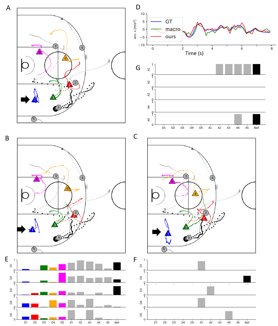
Table 1 (left) shows our three constraint losses. Our method (VRNN-Mech) shows smaller losses than the conventional method (VRNN). Although our partial observation model (VRNN-Bi) shows losses similar to or larger than those of the baseline models (VRNN and VRNN-macro), our full model (VRNN-macro-Bi-Mech) shows smaller losses than they do. Our model generated more physically plausible and smoother trajectories. For example, regarding , Fig. 3D shows examples of acceleration sequences for defender 1 (blue in Fig. 3A). Our model (red) generated smoother accelerations like the ground truth (blue) than VRNN-macro (green). The detailed analyses with mechanical constraints are described in Appendix F.
| Basketball data | Soccer data | |||||
| Position | Velocity | Acceleration | Position | Velocity | Acceleration | |
| Velocity | ||||||
| RNN-Gauss | ||||||
| VRNN | ||||||
| VRNN-macro | ||||||
| VRNN-Mech | ||||||
| VRNN-Bi | ||||||
| VRNN-macro-Bi-Mech | ||||||
5.2.2 Trajectory prediction performances
Table 2 (left) shows trajectory prediction performances. We confirmed the competitive long-term prediction of our mechanical constraints (VRNN-Mech) compared with the baseline models (VRNN and VRNN-macro). Note that our three mechanical constraints nonlinearly influence each other and do not always improve the prediction performance (it is not the main purpose). Our observation models (VRNN-Bi and VRNN-macro-Bi-Mech) show prediction performances similar to those of the baselines regardless of the partial observation.
Additionally, we also report the trajectory prediction performance of dNRI in the same setup. The smallest prediction errors were , , and for position, velocity, and acceleration, respectively. These performances were worse than for Velocity or RNN-Gauss, but the purpose of dNRI was not long-term prediction. The detailed analyses with mechanical constraints, discussion about VRNN-macro, and the overall mean prediction errors are described in Appendices F, D, and H, respectively.
5.2.3 Evaluation of observation model
We visually and quantitatively evaluated VRNN-macro-Bi-Mech. The averaged observation coefficient (i.e., binary vector ) was for each player (maximum 11). That for dNRI (i.e., relation) was . Fig. 3E (at the moment with larger marks in Fig. 3B) shows that the defenders observed both near and far players (for the sequences for , see Appendix I).
Meanwhile, there was no relation for five defenders inferred by dNRI at the same timestamp (instead, we show the relation for five attackers in Fig. 3G). Compared with our methods, dNRI extracted fewer relations or observations focusing on a specific person such as in Fig. 3G. Quantitatively, the ratio of no relation for each defender is , which is too large to analyze defenders’ observations (that of no observation in our method is ). Note that since there is no ground truth of human observations or relations, accurate evaluation among methods would be difficult currently.
Our model, which can predict long-term behaviors and model observations with a large variation (near and far agents for each agent), can analyze real-world multi-agent behaviors. For example, defender 1 (arrow) in Figs. 3A and B adopted the balanced position between attacker 1 and other attackers to help teammates near the ball (black). Our model can also create a counterfactual example when is artificially set to a one-hot vector at each moment (only the player highest in ) in Figs. 3C and F. In this case, like sports beginners, defender 1 went to the nearest attacker (attacker 1), and ignored the ball. Our model can analyze such behaviors in real-world agents. Additional analysis to compare the distances in observation among our method, dNRI, and a simple rule-based model is described in Appendix I.
5.3 Soccer data
To demonstrate the generality of our approach, we also used a soccer dataset [Le et al.,, 2017, Yeh et al.,, 2019], containing trajectories of soccer players and the ball from 45 professional soccer league games. We randomly split the dataset into 21504 training sequences, 2165 validation sequences, and 2452 test sequences. We did not model the goalkeepers since they tend to move very little. Table 1 (right) and Table 2 (right) indicate the effectiveness of our mechanical constraints and the similar trajectory prediction performance of our binary observation models and the baselines, results that were similar to those for the basketball dataset. For VRNN-macro-Bi-Mech, the averaged was for each defender (maximum 23). The ratio of no relation for each defender in our method is . Additional analysis to compare the distances in observation and an illustrative example are given in Appendices I and J, respectively.
6 Conclusions
We proposed decentralized policy models with partial observation and mechanical constraints. Using real-world basketball and soccer datasets, we show the effectiveness of our method in terms of the constraint violations, long-term prediction, and partial observation. Our approach can be used as a multi-agent simulator to generate realistic trajectories using real-world data. One possible future research direction is to incorporate other physiological constraints into the models such as visuomotor delays and body loads, which will contribute to the understanding of smooth multi-agent behaviors in complex environments.
Acknowledgments
This work was supported by Japan Society for the Promotion of Science KAKENHI (grant numbers 19H04941 and 23H03282) and Japan Science and Technology Agency PRESTO (grant number JPMJPR20CA).
Appendix A Observation in multi-agent systems.
In purely rule-based models, researchers investigating animals and vehicles conventionally proposed predefined observation rules based on specific distances and visual angles (e.g., Couzin et al., [2002]), the specific number of the nearest agents (e.g., Ballerini et al., [2008]), or other environments (e.g., Yoshihara et al., [2017]). However, it is difficult to define interactions between agents using predefined rules in general large-scale multi-agent systems. Thus, methods for learning observation of agents have been proposed for MARL in virtual environments [Mao et al.,, 2019, Jiang and Lu,, 2018, Iqbal and Sha,, 2019, Liu et al.,, 2020] and for real-world multi-agent systems [Hoshen,, 2017, Leurent and Mercat,, 2019, Guangyu et al.,, 2020, Fujii et al.,, 2020].
Here we introduce several approaches for neural network-based partial observation using soft and hard attention mechanisms, and other approaches. Note that we finally aim to model a multi-hot observation in decentralized biological multi-agent systems that can also predict long-term behaviors.
Attention is widely used in natural language processing [Bahdanau et al.,, 2014], computer vision [Wang et al.,, 2018], and MARL in virtual environments [Mao et al.,, 2019, Jiang and Lu,, 2018, Iqbal and Sha,, 2019]. Soft attention calculates an importance distribution of elements (e.g., agents): , where is a scalar variable for an agent . Soft attention is fully differentiable and thus can be trained with back-propagation. However, it usually assigns nonzero probabilities to unrelated elements; i.e., it cannot directly reduce the number of agents.
Hard attention focuses solely on an important element but is basically nondifferentiable because of the selection based on sampling. Among differentiable models with discrete variables, an approach using Gumbel-softmax reparameterization [Jang et al.,, 2017, Maddison et al.,, 2017] can be effectively implemented via a continuous relaxation of a discrete categorical distribution. In summary, given -categorical distribution parameters , a differentiable -dimensional one-hot encoding sample from the Gumbel-softmax distribution can be computed as: where are independent identically distributed samples from a Gumbel distribution, i.e., . is a uniform distribution and is the softmax temperature parameter. However, the resulting one-hot vector is insufficient to represent a multi-hot observation.
Appendix B Role assignment problem
In most real-world data, training (i.e., demonstration) data and test data include sequences from different types of agent (e.g., teams and games). Learning policies based on players’ positions or roles, instead of identity, seems to be more natural and more data-efficient in general. Among several approaches [Le et al.,, 2017, Yeh et al.,, 2019], for the behavioral modeling in a POMDP, we separate the problem into role assignment problem and policy learning based on [Le et al.,, 2017].
The unstructured set of demonstrations is denoted by , where is the sequence of actions by agent at time . Let be the context associated with each demonstration sequence (e.g., an opponent team and ball). In a role assignment problem, the indexing mechanism is formulated as an assignment function that maps the unstructured set and some probabilistic structured model to an indexed set of states rearranged from ; i.e.,
where the set . We consider as a latent variable model that infers the role assignments for each set of demonstrations. The role assignment with a latent structured model addresses two main issues: (1) unsupervised learning of a probabilistic role assignment model ; and (2) the indexing with so that unstructured sequences can be mapped to structured sequences.
First, in the unsupervised learning of the stochastic role assignment model, we use a Gaussian hidden markov model (Gaussian HMM) according to [Le et al.,, 2017]. The Gaussian HMM inputs a state feature vector defined by all agents’ information and learn transition probabilities and Gaussian mixture distributions as output probabilities of hidden states.
Second, for indexing based on to map to , we solve a well-known linear assignment problem [Papadimitriou and Steiglitz,, 1982]. Concretely, the distance between the mixed Gaussian distribution obtained above and the state feature vector is computed for each time and each player. The linear assignment problem is then solved with use of the distance as a cost function (i.e., roles are assigned in order of players whose distance is closer to each Gaussian distribution).
Appendix C Variational recurrent neural networks
Here we briefly overview RNNs, VAEs, and VRNNs.
From the perspective of a probabilistic generative model, an RNN models the conditional probabilities with a hidden state that summarizes the history in the first timesteps:
| (4) |
where maps the hidden state to a probability distribution over states and is a deterministic function such as LSTMs or gated recurrent units (GRUs). RNNs with simple output distributions often struggle to capture highly variable and structured sequential data. Recent work in sequential generative models addressed this issue by injecting stochastic latent variables into the model and using amortized variational inference to infer latent variables from data. A VRNN [Chung et al.,, 2015] is one of the methods using this idea and combining RNNs and VAEs.
A VAE [Kingma and Welling,, 2014] is a generative model for nonsequential data that injects latent variables into the joint distribution and introduces an inference network parameterized by to approximate the posterior . The learning objective is to maximize the ELBO of the log-likelihood with respect to the model parameters and :
| (5) |
. The first term is known as the reconstruction term and can be approximated with Monte Carlo sampling. The second term is the KL divergence between the approximate posterior and the prior, and can be evaluated analytically if both distributions are Gaussian with diagonal covariance. The inference model , generative model , and prior are often implemented with neural networks.
VRNNs combine VAEs and RNNs by conditioning the VAE on a hidden state :
| (prior) | (6) | ||||
| (inference) | (7) | ||||
| (generation) | (8) | ||||
| (recurrence) | (9) |
VRNNs are also trained by maximizing the ELBO, which can be interpreted as the sum of VAE ELBOs over each timestep of the sequence:
| (10) | ||||
Note that the prior distribution of latent variable depends on the history of states and latent variables (Eq. (6)).
Appendix D Decentralized and partially observed macro goals
Our model uses macro goal [Zhan et al.,, 2019] for long-term prediction by modifying our decentralized and partially observable setting. Here we briefly review the original macro goal and describe our modification of the decentralized and partially observable setting. We also discuss the related results of our experiments.
As an illustrative example, Fig. 2B shows macro goals for a basketball defender as specific areas on the court (boxes). After reaching the macro goal in the center, the blue player moves towards the next macro goal at the top (middle). The macro goals provide a compact summary of the players’ sequences over a long time to encode long-term intent.
D.1 Shared macro goals
The original macro goal or macro intent [Zheng et al.,, 2016, Zhan et al.,, 2019], obtained via some labeling functions, is defined as low-dimensional and spatiotemporal representations of the data for the learning of multi-agent long-term coordination such as basketball (Figure 2B). The original macro goal assumes that: (1) it provides a tractable way to capture coordination between agents; (2) it encodes long-term goals of agents and enables long-term planning at a higher-level timescale; and (3) it compactly represents some low-dimensional structure in an exponentially large multi-agent state space.
Specifically, the modeling assumptions for the original macro goals are as follows: 1) agent states in a period are conditioned on some shared macro goal ; 2) the start and end times of episodes can vary between sequences; 3) macro goals change slowly over time relative to the agent states: , and 4) due to their reduced dimensionality, (near-) arbitrary dependencies between macro goals (e.g., coordination) can be modeled by a neural network approach.
Among various labeling approaches (see [Zhan et al.,, 2019]) for the macro goal, programmatic weak supervision is a method requiring low labor cost, effectively learning the underlying structure of large unlabeled datasets, and allowing users to incorporate domain knowledge into the model. For example, the labeling function to obtain macro goals for basketball sequences computes the regions on the court in which players remain stationary; this integrates the idea that players aim to set up specific formations on the court.
Specifically, previous work labeled the macro goal independently among agents (obtained in a rule based manner), and learned the shared macro goal model via supervised learning by maximizing the log-likelihood of macro goal labels. The model finally returns the one-hot encoding of the box that contains the position information.
D.2 Specific setup in our experiments
Our decentralized and partially observed macro goals (1) use partial observation to obtain the macro goal model and (2) independently learn the decentralized macro goal (not shared between agents). Among several labeling functions, we adopted the stationary labeling function to compute the macro goal on the basis of stationary positions because it reflects important information about the structure of the data, and its better performance was confirmed [Zhan et al.,, 2019].
For basketball data, according to the previous work [Zhan et al.,, 2019], we define the macro goal by segmenting the left half-court into a grid of boxes (Fig. 2B). For soccer data, we segmented the total court into a grid of approximately boxes.
D.3 Related discussion in our experiments
We confirmed the decentralized and partially observed macro goals did not improve the prediction performances. There are mainly two reasons for this. One is obviously the decentralized (i.e., not shared) setting, but it is a necessary assumption for our modeling. The second is the improvement of the VRNN baseline by our adding dropout and batch normalization layers to avoid overfitting (note that they were added in all models for fair comparisons). Specifically in the soccer experiment, the resolution of the grid might make it larger than that of the prediction (but the smaller grid might be difficult to learn the macro goal).
Appendix E Training details
Here we describe a specific objective function in our experiments, and other training details. For other implementation details, such as preprocessing including role assignment in B, see the code at https://github.com/keisuke198619/PO-MC-DHVRNN.
E.1 Objective function in our experiments
We designed the objective function as described in Section 3.4, but we specially weighted each term of the objective function. Note that, in our experiments, we selected velocity and acceleration as the output actions (see G). In this case, the penalty for the predicted dimension and the eliminated dimension can be computed only for acceleration and only for position, respectively. That is, the weighted penalties of the mechanical constraints are
| (11) | |||
where , , and are regularization parameters. As shown in F, the first and second terms improved the prediction performance of velocity and position, respectively (the third term basically contributed to smoothing in acceleration as shown in Fig. 3D). The results also show that the learning of acceleration was relatively difficult because of the above-mentioned imbalance between the dimensions. We then added the reconstruction term in only for acceleration. In summary, the specific objective function in our experiments was . We set , , , and in the basketball experiment and , , , and in the soccer experiment, because the trajectories in the soccer dataset were more difficult to predict than those in the basketball dataset as shown in Table 2 (i.e., the reconstruction was prioritized).
E.2 Other training details
We trained all the models using the Adam optimizer [Kingma and Ba,, 2015] with default parameters using teacher forcing [Williams and Zipser,, 1989]. To prevent overfitting, dropout and batch normalization layers were used (the dropout rate was set to 0.5), and we selected the model with the best performance on the validation set. We set the embedding dimension to for each agent (and the ball). The embedding layer, the macro goal decoder , prior , encoder , and decoder in the VRNN were implemented by a two-layer neural network with a hidden layer of size . We modeled each latent variable as a multivariate Gaussian with diagonal covariance of dimension . All GRUs were implemented by a two-layer neural network with a hidden layer of size . Other implementations were based on [Zhan et al.,, 2019]. We selected position, velocity, and acceleration as the input states (i.e., ). The reason for and the analysis of various input states and output actions are described in G. For the temperature in a Gumbel-softmax distribution, we set it to in both experiments.
The VRNN decoder was implemented by a two-layer neural network returning a multivariate Gaussian with diagonal covariance. The original VRNN [Chung et al.,, 2015] has no constraint in the learning of the variance. It may cause the NLL to tend toward infinity when the variance approaches zero. Most of the cases, including our experiments, such problems did not happen (in such difficult cases, setting the decoder variance as a global hyperparameter will be practically effective). In our model, the KL divergence in the first term in Eq. (3) includes , where is the directly estimated variance, and the term may prevent the variance from approaching zero.
E.3 Training in dNRI
Additionally, we also investigated dNRI [Graber and Schwing,, 2020] as a baseline, which infers dynamic relation as a variant of NRI [Kipf et al.,, 2018], based on the same setting (2-s burn-in and 6-s prediction of five defenders) using the basketball dataset. The batch size was 32, and the other hyperparameters were the same as in previous work [Graber and Schwing,, 2020]. Note that our methods modeled five defenders independently, but dNRI modeled all agents and the ball (i.e., regarding five attackers and the ball, the ground-truth data is used also in the test prediction phase). Therefore, dNRI can infer the attackers’ (and the ball’s) relations, such as in Fig. 3G.
Appendix F Analysis of mechanical constraints
Here we verify various mechanical constraints in our model. The detailed objective function was described in E. For clarity, we evaluated the prediction performance of the VRNN using the basketball data among various options: (1) VRNN, (2) VRNN-, (3) VRNN-, (4) VRNN-, and (5) VRNN-- (VRNN-Mech in the main text). The second, third, and fourth options added the penalty of the second, first, and third terms in Eq. (11), respectively. The fifth option added the acceleration reconstruction term .
Table 3 gives the results for the constraint losses for the basketball dataset. Obviously, , , and improved by addition of , , and , respectively. When was added, (and the prediction of acceleration below) improved but became worse. In other words, there was a trade-off between and the prediction of acceleration.
| (NLL) | (KLD) | (NLL) | |
| VRNN | 242.44 25.25 | 3.70 0.22 | 134.37 10.01 |
| VRNN- | 124.83 15.87 | 4.01 0.17 | 115.78 9.62 |
| VRNN- | 162.29 18.60 | 3.69 0.17 | 111.03 8.53 |
| VRNN- | 156.05 18.28 | 3.69 0.17 | 107.22 8.13 |
| VRNN-- | 130.81 15.46 | 3.44 0.19 | 124.40 8.83 |
Table 4 gives the results for prediction performances. slightly improved the prediction performance of velocity ( basically contributed to smoothing in acceleration as shown in Fig. 3D). The results also show that the learning of acceleration was relatively difficult because of the above-mentioned imbalance between the dimensions. We thus added the reconstruction term . VRNN-- (VRNN-Mech in the main text) shows better prediction performance in all dimensions.
| Average | Smallest | |||||
| Position | Velocity | Acceleration | Position | Velocity | Acceleration | |
| VRNN | ||||||
| VRNN- | ||||||
| VRNN- | ||||||
| VRNN- | ||||||
| VRNN-- | 0.10 | 0.21 | ||||
Appendix G Analysis of input state and output action dimensions
Here we verify various options to select input state and output action dimensions among position, velocity, and acceleration. The action in previous studies (e.g., Zhan et al., [2019], Yeh et al., [2019]) was usually the agent’s position, but these studies reported the difficulty in learning velocity and acceleration (e.g., change in direction of movement), which is critical in our problem. We aim to obtain policy models to generate biologically realistic actions in terms of position, velocity, and acceleration.
For simplicity, we evaluated the prediction performance of the VRNN using the basketball data among various options: (1) VRNN-pos, (2) VRNN-vel, (3) VRNN-acc, (4) VRNN-pos-vel-acc, and (5) VRNN-vel-acc. The first one uses only positional information as the input and output as the baseline as used in most of the previous studies (e.g., Zhan et al., [2019], Yeh et al., [2019]). The second one uses position and velocity as the input and only velocity as the output for comparison with VRNN-pos and VRNN-vel-acc. The remaining ones use the full information (position, velocity, and acceleration) as the input. The third and fourth ones use only acceleration and the full information as the output, respectively, for comparison with VRNN-vel-acc. The fifth one uses velocity and acceleration as the output. The second, third, and fifth ones compute the future positions using the current position and velocity (the third similarly computes velocity).
Table 5 gives the results of the analysis. The model effectively learned the dimension of the output (e.g., position in VRNN-pos) but the indirect learning of the differential value (e.g., velocity) was difficult. In contrast, for the indirect learning of the integral value, the learning of position using velocity was effective, but the learning of velocity using acceleration was difficult. This may be caused by the data having noisy accelerations. The specific difficulty in numerical differentiation and integration, which is considered as a hard constraint in Section 3.3, derived possibly from the low spatiotemporal resolution of the data. The learning of all dimensions (VRNN-pos-vel-acc) did not show better performance in all dimensions. VRNN-vel-acc shows better prediction performance in all dimensions. Therefore, we chose VRNN-vel-acc as our base model.
| Average | Smallest | |||||
| Position | Velocity | Acceleration | Position | Velocity | Acceleration | |
| VRNN-pos | ||||||
| VRNN-vel | ||||||
| VRNN-acc | ||||||
| VRNN-pos-vel-acc | 0.18 | |||||
| VRNN-vel-acc (main) | ||||||
Appendix H Supplemental results of prediction error
The average prediction errors in Table 6 indicate similar tendencies as the smallest prediction errors in Table 2.
Additionally, we also examined dNRI [Graber and Schwing,, 2020]. The average prediction errors were , and in position, velocity, and acceleration, respectively. These performances were worse than for Velocity or RNN-Gauss, but the purpose of dNRI (and variants of NRI) was not long-term prediction.
| Basketball data | Soccer data | |||||
| Position | Velocity | Acceleration | Position | Velocity | Acceleration | |
| Velocity | ||||||
| RNN-Gauss | ||||||
| VRNN | ||||||
| VRNN-macro | ||||||
| VRNN-Mech | ||||||
| VRNN-Bi | ||||||
| VRNN-macro-Bi-Mech | ||||||
Appendix I Additional analysis of observations
To compare our method with a simple rule-based model, we computed three distances between the subject player and the furthest player observed in our model, dNRI, and a rule-based model. The last considered the same-order nearest player as the number of players observed in our model and dNRI (different numbers), which is considered to be determined by a compatible and well-known predetermined rule [Ballerini et al.,, 2008]. The mean distance from the furthest player in our model was greater than that of the same-order nearest player ( and ). In dNRI, it was relatively greater than that of the same-order nearest player ( and ). Our model and dNRI reflected far agent information (but we ignored no-relation sequences in dNRI). For example, defender 1 (arrow) in Figs. 3A and B adopted the balanced position between attacker 1 and other attackers to help teammates near the ball (black).
In the soccer dataset, our model reflected far agent information (the mean distance in our model was and that in the same-order nearest player was ).
Next, we show example sequences of the observation coefficients in Figs. 4A, B, and D, which correspond to defender 1’s observation coefficients in Figs. 3E, F, and G (our normal prediction, our counterfactual prediction, and the dNRI prediction for the basketball dataset), respectively. Fig. 4C shows the defender 1’s relation inferred by dNRI, but at the moment in Fig. 3 (), there was no observation. We confirmed that the observation coefficients for the ball and the nearest attacker (attacker 1) were higher than for other players in Figs. 4A and B. The defender’s relation extracted by dNRI in Fig. 4C was sparser than for our observation model in Fig. 4A, whereas the attacker’s relation in Fig. 4D was dense. However, quantitatively, the ratio of no relation for each attacker in dNRI is , which is a level similar to that for each defender described in Section 4.2.

Appendix J Evaluation results and an illustrative example using the soccer dataset
We obtained an example for VRNN-macro-Bi-Mech using the soccer dataset in Fig. 5. Unlike the basketball example in Fig. 3, the ground truth and a normal prediction in Figs. 5A and B were similar, possibly because the soccer pitch () was larger than the basketball half-court (). For the observation model, the results for a normal prediction in Fig. 5C indicate that defender 1 observed specific players and the ball.

References
- Alahi et al., [2016] Alahi, A., Goel, K., Ramanathan, V., Robicquet, A., Fei-Fei, L., and Savarese, S. (2016). Social lstm: Human trajectory prediction in crowded spaces. In Proceedings of the IEEE Conference on Computer Vision and Pattern Recognition, pages 961–971.
- Amato et al., [2019] Amato, C., Konidaris, G., Kaelbling, L. P., and How, J. P. (2019). Modeling and planning with macro-actions in decentralized pomdps. Journal of Artificial Intelligence Research, 64:817–859.
- Bahdanau et al., [2014] Bahdanau, D., Cho, K., and Bengio, Y. (2014). Neural machine translation by jointly learning to align and translate. arXiv preprint arXiv:1409.0473.
- Ballerini et al., [2008] Ballerini, M., Cabibbo, N., Candelier, R., Cavagna, A., Cisbani, E., Giardina, I., Lecomte, V., Orlandi, A., Parisi, G., Procaccini, A., et al. (2008). Interaction ruling animal collective behavior depends on topological rather than metric distance: Evidence from a field study. Proceedings of the National Academy of Sciences, 105(4):1232–1237.
- Bansal et al., [2018] Bansal, M., Krizhevsky, A., and Ogale, A. (2018). Chauffeurnet: Learning to drive by imitating the best and synthesizing the worst. arXiv preprint arXiv:1812.03079.
- Becker et al., [2018] Becker, S., Hug, R., Hübner, W., and Arens, M. (2018). Red: A simple but effective baseline predictor for the trajnet benchmark. In European Conference on Computer Vision, pages 138–153. Springer.
- Bernstein et al., [2002] Bernstein, D. S., Givan, R., Immerman, N., and Zilberstein, S. (2002). The complexity of decentralized control of markov decision processes. Mathematics of Operations Research, 27(4):819–840.
- [8] Chen, C.-Y., Lai, W., Hsieh, H.-Y., Zheng, W.-H., Wang, Y.-S., and Chuang, J.-H. (2018a). Generating defensive plays in basketball games. In Proceedings of the 26th ACM International Conference on Multimedia, pages 1580–1588.
- [9] Chen, T. Q., Rubanova, Y., Bettencourt, J., and Duvenaud, D. K. (2018b). Neural ordinary differential equations. In Advances in Neural Information Processing Systems 31, pages 6571–6583.
- Chung et al., [2015] Chung, J., Kastner, K., Dinh, L., Goel, K., Courville, A. C., and Bengio, Y. (2015). A recurrent latent variable model for sequential data. In Advances in Neural Information Processing Systems 28, pages 2980–2988.
- Cichy and Kaiser, [2019] Cichy, R. M. and Kaiser, D. (2019). Deep neural networks as scientific models. Trends in Cognitive Sciences, 23(4):305–317.
- Couzin et al., [2002] Couzin, I. D., Krause, J., James, R., Ruxton, G. D., and Franks, N. R. (2002). Collective memory and spatial sorting in animal groups. Journal of Theoretical Biology, 218(1):1–11.
- Dias et al., [2020] Dias, C., Iryo-Asano, M., Abdullah, M., Oguchi, T., and Alhajyaseen, W. (2020). Modeling trajectories and trajectory variation of turning vehicles at signalized intersections. IEEE Access, 8:109821–109834.
- Eyjolfsdottir et al., [2017] Eyjolfsdottir, E., Branson, K., Yue, Y., and Perona, P. (2017). Learning recurrent representations for hierarchical behavior modeling. In International Conference on Learning Representations.
- Flash and Hogan, [1985] Flash, T. and Hogan, N. (1985). The coordination of arm movements: an experimentally confirmed mathematical model. Journal of Neuroscience, 5(7):1688–1703.
- Fraccaro et al., [2017] Fraccaro, M., Kamronn, S., Paquet, U., and Winther, O. (2017). A disentangled recognition and nonlinear dynamics model for unsupervised learning. In Advances in Neural Information Processing Systems 30, pages 3601–3610.
- Fraccaro et al., [2016] Fraccaro, M., Sønderby, S. K., Paquet, U., and Winther, O. (2016). Sequential neural models with stochastic layers. In Advances in Neural Information Processing Systems 29, pages 2199–2207.
- Fujii, [2021] Fujii, K. (2021). Data-driven analysis for understanding team sports behaviors. Journal of Robotics and Mechatronics, 33(3):505–514.
- [19] Fujii, K., Isaka, T., Kouzaki, M., and Yamamoto, Y. (2015a). Mutual and asynchronous anticipation and action in sports as globally competitive and locally coordinative dynamics. Scientific Reports, 5.
- Fujii and Kawahara, [2019] Fujii, K. and Kawahara, Y. (2019). Dynamic mode decomposition in vector-valued reproducing kernel hilbert spaces for extracting dynamical structure among observables. Neural Networks, 117:94–103.
- Fujii et al., [2020] Fujii, K., Takeishi, N., Hojo, M., Inaba, Y., and Kawahara, Y. (2020). Physically-interpretable classification of network dynamics for complex collective motions. Scientific Reports, 10(3005):1–13.
- Fujii et al., [2019] Fujii, K., Takeishi, N., Kibushi, B., Kouzaki, M., and Kawahara, Y. (2019). Data-driven spectral analysis for coordinative structures in periodic human locomotion. Scientific Reports, 9(1):1–14.
- Fujii et al., [2021] Fujii, K., Takeishi, N., Tsutsui, K., Fujioka, E., Nishiumi, N., Tanaka, R., Fukushiro, M., Ide, K., Kohno, H., Yoda, K., et al. (2021). Learning interaction rules from multi-animal trajectories via augmented behavioral models. Advances in Neural Information Processing Systems, 34:11108–11122.
- Fujii et al., [2022] Fujii, K., Takeuchi, K., Kuribayashi, A., Takeishi, N., Kawahara, Y., and Takeda, K. (2022). Estimating counterfactual treatment outcomes over time in complex multi-agent scenarios. arXiv preprint arXiv:2206.01900.
- Fujii et al., [2016] Fujii, K., Yokoyama, K., Koyama, T., Rikukawa, A., Yamada, H., and Yamamoto, Y. (2016). Resilient help to switch and overlap hierarchical subsystems in a small human group. Scientific Reports, 6(1):1–10.
- [26] Fujii, K., Yoshioka, S., Isaka, T., and Kouzaki, M. (2015b). The preparatory state of ground reaction forces in defending against a dribbler in a basketball 1-on-1 dribble subphase. Sports Biomechanics, 14(1):28–44.
- Goyal et al., [2017] Goyal, A. G. A. P., Sordoni, A., Côté, M.-A., Ke, N. R., and Bengio, Y. (2017). Z-forcing: Training stochastic recurrent networks. In Advances in Neural Information Processing Systems 30, pages 6713–6723.
- Graber and Schwing, [2020] Graber, C. and Schwing, A. G. (2020). Dynamic neural relational inference. In Proceedings of the IEEE/CVF Conference on Computer Vision and Pattern Recognition (CVPR).
- Guangyu et al., [2020] Guangyu, L., Bo, J., Hao, Z., Zhengping, C., and Yan, L. (2020). Generative attention networks for multi-agent behavioral modeling. In Thirty-Fourth AAAI Conference on Artificial Intelligence.
- Gupta et al., [2018] Gupta, A., Johnson, J., Fei-Fei, L., Savarese, S., and Alahi, A. (2018). Social gan: Socially acceptable trajectories with generative adversarial networks. In Proceedings of the IEEE Conference on Computer Vision and Pattern Recognition, pages 2255–2264.
- Helbing and Molnar, [1995] Helbing, D. and Molnar, P. (1995). Social force model for pedestrian dynamics. Physical Review E, 51(5):4282.
- Hoshen, [2017] Hoshen, Y. (2017). Vain: Attentional multi-agent predictive modeling. In Advances in Neural Information Processing Systems 30, pages 2701–2711.
- Hsieh et al., [2019] Hsieh, H.-Y., Chen, C.-Y., Wang, Y.-S., and Chuang, J.-H. (2019). Basketballgan: Generating basketball play simulation through sketching. In Proceedings of the 27th ACM International Conference on Multimedia, pages 720–728.
- Iqbal and Sha, [2019] Iqbal, S. and Sha, F. (2019). Actor-attention-critic for multi-agent reinforcement learning. In International Conference on Machine Learning, pages 2961–2970.
- Ivanovic et al., [2018] Ivanovic, B., Schmerling, E., Leung, K., and Pavone, M. (2018). Generative modeling of multimodal multi-human behavior. In 2018 IEEE/RSJ International Conference on Intelligent Robots and Systems, pages 3088–3095. IEEE.
- Jang et al., [2017] Jang, E., Gu, S., and Poole, B. (2017). Categorical reparametrization with gumble-softmax. In International Conference on Learning Representations. OpenReview. net.
- Jiang and Lu, [2018] Jiang, J. and Lu, Z. (2018). Learning attentional communication for multi-agent cooperation. In Advances in Neural Information Processing Systems 31, pages 7254–7264.
- Johnson et al., [2016] Johnson, M. J., Duvenaud, D. K., Wiltschko, A., Adams, R. P., and Datta, S. R. (2016). Composing graphical models with neural networks for structured representations and fast inference. In Advances in Neural Information Processing Systems 29, pages 2946–2954.
- Kaelbling et al., [1998] Kaelbling, L. P., Littman, M. L., and Cassandra, A. R. (1998). Planning and acting in partially observable stochastic domains. Artificial Intelligence, 101(1-2):99–134.
- Karl et al., [2017] Karl, M., Soelch, M., Bayer, J., and van der Smagt, P. (2017). Deep variational bayes filters: Unsupervised learning of state space models from raw data. In International Conference on Learning Representations.
- Khanna and Tan, [2019] Khanna, S. and Tan, V. Y. (2019). Economy statistical recurrent units for inferring nonlinear granger causality. In International Conference on Learning Representations.
- Kingma and Ba, [2015] Kingma, D. P. and Ba, J. (2015). Adam: A method for stochastic optimization. In International Conference on Learning Representations.
- Kingma and Welling, [2014] Kingma, D. P. and Welling, M. (2014). Auto-encoding variational bayes. In International Conference on Learning Representations.
- Kipf et al., [2018] Kipf, T., Fetaya, E., Wang, K.-C., Welling, M., and Zemel, R. (2018). Neural relational inference for interacting systems. In International Conference on Machine Learning, pages 2688–2697.
- Le et al., [2017] Le, H. M., Yue, Y., Carr, P., and Lucey, P. (2017). Coordinated multi-agent imitation learning. In Proceedings of the 34th International Conference on Machine Learning-Volume 70, pages 1995–2003.
- Leurent and Mercat, [2019] Leurent, E. and Mercat, J. (2019). Social attention for autonomous decision-making in dense traffic. arXiv preprint arXiv:1911.12250.
- Liu et al., [2019] Liu, A. T., Hsu, P.-c., and Lee, H.-Y. (2019). Unsupervised end-to-end learning of discrete linguistic units for voice conversion. Proc. Interspeech 2019, pages 1108–1112.
- Liu et al., [2020] Liu, Y., Wang, W., Hu, Y., Hao, J., Chen, X., and Gao, Y. (2020). Multi-agent game abstraction via graph attention neural network. In Thirty-Fourth AAAI Conference on Artificial Intelligence 34, volume 34, pages 7211–7218.
- Löwe et al., [2020] Löwe, S., Madras, D., Zemel, R., and Welling, M. (2020). Amortized causal discovery: Learning to infer causal graphs from time-series data. arXiv preprint arXiv:2006.10833.
- Maddison et al., [2017] Maddison, C. J., Mnih, A., and Teh, Y. W. (2017). The concrete distribution: A continuous relaxation of discrete random variables. In International Conference on Learning Representations.
- Mao et al., [2019] Mao, H., Zhang, Z., Xiao, Z., and Gong, Z. (2019). Modelling the dynamic joint policy of teammates with attention multi-agent ddpg. In Proceedings of the 18th International Conference on Autonomous Agents and MultiAgent Systems, pages 1108–1116.
- Papadimitriou and Steiglitz, [1982] Papadimitriou, C. H. and Steiglitz, K. (1982). Combinatorial optimization, volume 24. Prentice Hall Englewood Cliffs.
- Pham et al., [2007] Pham, Q.-C., Hicheur, H., Arechavaleta, G., Laumond, J.-P., and Berthoz, A. (2007). The formation of trajectories during goal-oriented locomotion in humans. ii. a maximum smoothness model. European Journal of Neuroscience, 26(8):2391–2403.
- Rainforth et al., [2018] Rainforth, T., Kosiorek, A., Le, T. A., Maddison, C., Igl, M., Wood, F., and Teh, Y. W. (2018). Tighter variational bounds are not necessarily better. In International Conference on Machine Learning, volume 80, pages 4277–4285.
- Rhinehart et al., [2019] Rhinehart, N., McAllister, R., Kitani, K., and Levine, S. (2019). Precog: Prediction conditioned on goals in visual multi-agent settings. In Proceedings of the IEEE International Conference on Computer Vision, pages 2821–2830.
- Ross et al., [2011] Ross, S., Gordon, G., and Bagnell, D. (2011). A reduction of imitation learning and structured prediction to no-regret online learning. In Proceedings of the fourteenth International Conference on Artificial Intelligence and Statistics, pages 627–635.
- Rupprecht et al., [2017] Rupprecht, C., Laina, I., DiPietro, R., Baust, M., Tombari, F., Navab, N., and Hager, G. D. (2017). Learning in an uncertain world: Representing ambiguity through multiple hypotheses. In Proceedings of the IEEE International Conference on Computer Vision, pages 3591–3600.
- Schaal, [1996] Schaal, S. (1996). Learning from demonstration. Advances in Neural Information Processing Systems, 9:1040–1046.
- Sun et al., [2019] Sun, C., Karlsson, P., Wu, J., Tenenbaum, J. B., and Murphy, K. (2019). Predicting the present and future states of multi-agent systems from partially-observed visual data. In International Conference on Learning Representations.
- Tang and Salakhutdinov, [2019] Tang, C. and Salakhutdinov, R. R. (2019). Multiple futures prediction. In Advances in Neural Information Processing Systems 32, pages 15398–15408.
- Tank et al., [2018] Tank, A., Covert, I., Foti, N., Shojaie, A., and Fox, E. (2018). Neural granger causality for nonlinear time series. arXiv preprint arXiv:1802.05842.
- Teranishi et al., [2020] Teranishi, M., Fujii, K., and Takeda, K. (2020). Trajectory prediction with imitation learning reflecting defensive evaluation in team sports. In 2020 IEEE 9th Global Conference on Consumer Electronics (GCCE), pages 124–125. IEEE.
- Teranishi et al., [2022] Teranishi, M., Tsutsui, K., Takeda, K., and Fujii, K. (2022). Evaluation of creating scoring opportunities for teammates in soccer via trajectory prediction. arXiv preprint arXiv:2206.01899.
- Tsutsui et al., [2021] Tsutsui, K., Fujii, K., Kudo, K., and Takeda, K. (2021). Flexible prediction of opponent motion with internal representation in interception behavior. Biological cybernetics, 115(5):473–485.
- Uno et al., [1989] Uno, Y., Kawato, M., and Suzuki, R. (1989). Formation and control of optimal trajectory in human multijoint arm movement. Biological Cybernetics, 61(2):89–101.
- Wang et al., [2018] Wang, X., Girshick, R., Gupta, A., and He, K. (2018). Non-local neural networks. In Proceedings of the IEEE Conference on Computer Vision and Pattern Recognition, pages 7794–7803.
- Williams and Zipser, [1989] Williams, R. J. and Zipser, D. (1989). A learning algorithm for continually running fully recurrent neural networks. Neural Computation, 1(2):270–280.
- Yeh et al., [2019] Yeh, R. A., Schwing, A. G., Huang, J., and Murphy, K. (2019). Diverse generation for multi-agent sports games. In Proceedings of the IEEE Conference on Computer Vision and Pattern Recognition, pages 4610–4619.
- Yoshihara et al., [2017] Yoshihara, Y., Morales, Y., Akai, N., Takeuchi, E., and Ninomiya, Y. (2017). Autonomous predictive driving for blind intersections. In 2017 IEEE/RSJ International Conference on Intelligent Robots and Systems (IROS), pages 3452–3459.
- Zhan et al., [2019] Zhan, E., Zheng, S., Yue, Y., Sha, L., and Lucey, P. (2019). Generating multi-agent trajectories using programmatic weak supervision. In International Conference on Learning Representations.
- Zheng et al., [2016] Zheng, S., Yue, Y., and Hobbs, J. (2016). Generating long-term trajectories using deep hierarchical networks. In Advances in Neural Information Processing Systems 29, pages 1543–1551.