Decentralized Optimization Over the Stiefel Manifold by an Approximate Augmented Lagrangian Function

Lei Wang State Key Laboratory of Scientific and Engineering Computing, Academy of Mathematics and Systems Science, Chinese Academy of Sciences, and University of Chinese Academy of Sciences, China ([email protected]). Research is supported by the National Natural Science Foundation of China (No. 11971466 and 11991020). Xin Liu State Key Laboratory of Scientific and Engineering Computing, Academy of Mathematics and Systems Science, Chinese Academy of Sciences, and University of Chinese Academy of Sciences, China ([email protected]). Research is supported in part by the National Natural Science Foundation of China (No. 12125108 and 11991021), Key Research Program of Frontier Sciences, Chinese Academy of Sciences (No. ZDBS-LY-7022).

Abstract

In this paper, we focus on the decentralized optimization problem over the Stiefel manifold, which is defined on a connected network of $d$ agents. The objective is an average of $d$ local functions, and each function is privately held by an agent and encodes its data. The agents can only communicate with their neighbors in a collaborative effort to solve this problem. In existing methods, multiple rounds of communications are required to guarantee the convergence, giving rise to high communication costs. In contrast, this paper proposes a decentralized algorithm, called DESTINY, which only invokes a single round of communications per iteration. DESTINY combines gradient tracking techniques with a novel approximate augmented Lagrangian function. The global convergence to stationary points is rigorously established. Comprehensive numerical experiments demonstrate that DESTINY has a strong potential to deliver a cutting-edge performance in solving a variety of testing problems.

1 Introduction

This paper is dedicated to providing an efficient approach to the decentralized optimization with orthogonality constraints, a problem defined on a connected network and solved by $d$ agents cooperatively.

	$\displaystyle\min\limits_{X\in\mathbb{R}^{n\times p}}$	$\displaystyle f(X):=\dfrac{1}{d}\sum\limits_{i=1}^{d}f_{i}(X)$		(1.1)
	$\displaystyle\mathrm{s.\,t.}$	$\displaystyle X^{\top}X=I_{p},$		(1.1)

where $I_{p}$ is the $p\times p$ identity matrix, and $f_{i}:\mathbb{R}^{n\times p}\to\mathbb{R}$ is a local function privately known by the $i$ -th agent. The set of all $n\times p$ orthogonal matrices is referred to as Stiefel manifold [37], which is denoted by $\mathcal{S}_{n,p}=\{X\in\mathbb{R}^{n\times p}\mid X^{\top}X=I_{p}\}$ . Throughout this paper, we make the following blanket assumptions about these local functions.

Assumption 1.

Each local objective function $f_{i}$ is smooth and its gradient $\nabla f_{i}$ is locally Lipschitz continuous.

We consider the scenario that the agents can only exchange information with their immediate neighbors through the network, which is modeled as a connected undirected graph $\mathtt{G}=(\mathtt{V},\mathtt{E})$ . Here, $\mathtt{V}=[d]:=\{1,2,\dotsc,d\}$ is composed of all the agents and $\mathtt{E}=\{(i,j)\mid i\text{~{}and~{}}j\text{~{}are connected}\}$ denotes the set of all the communication links. Let $X_{i}\in\mathbb{R}^{n\times p}$ be the local copy of the common variable $X$ kept by the $i$ -th agent. Then the optimization problem (1.1) over the Stiefel manifold can be equivalently recast as the following decentralized formulation.


$\displaystyle\min\limits_{\{X_{i}\}_{i=1}^{d}}\hskip 5.69054pt$	$\displaystyle\dfrac{1}{d}\sum\limits_{i=1}^{d}f_{i}(X_{i})$	(1.2a)
$\displaystyle\mathrm{s.\,t.}\,\,\hskip 7.11317pt$	$\displaystyle X_{i}=X_{j},\hskip 5.69054pt(i,j)\in\mathtt{E},$	(1.2b)
	$\displaystyle X_{i}\in\mathcal{S}_{n,p},\hskip 5.69054pti\in[d].$	(1.2c)

Since the graph $\mathtt{G}$ is assumed to be connected, the constraints (1.2b) enforce the consensus condition $X_{1}=X_{2}=\dotsb=X_{d}$ , which guarantees the equivalence between (1.1) and (1.2). Due to the nonconvexity of Stiefel manifolds, it is challenging to design efficient algorithms to solve (1.2).

1.1 Broad applications

Problems of the form (1.1) that require decentralized computations are found widely in various scientific and engineering areas. We briefly describe several representative applications of it below.

Application 1: Principal Component Analysis.

The principal component analysis (PCA) is a basic and ubiquitous tool for dimensionality reduction serving as a critical procedure or preprocessing step in numerous statistical and machine learning tasks. Mathematically, PCA amounts to solving the following optimization problem.

	$\displaystyle\min\limits_{X\in\mathbb{R}^{n\times p}}$	$\displaystyle-\frac{1}{2d}\sum\limits_{i=1}^{d}\mathrm{tr}\left(X^{\top}A_{i}A_{i}^{\top}X\right)$		(1.3)
	$\displaystyle\mathrm{s.\,t.}$	$\displaystyle X\in\mathcal{S}_{n,p},$		(1.3)

where $A=[A_{1},\dotsc,A_{d}]\in\mathbb{R}^{n\times m}$ is the data matrix consisting of $m$ samples with $n$ features. In the decentralized setting, $A_{i}\in\mathbb{R}^{n\times m_{i}}$ represents the local data stored in the $i$ -th agent such that $m=m_{1}+\dotsb+m_{d}$ . This is a natural scenario since each sample is a column of $A$ .

Application 2: Orthogonal Least Squares Regression.

The orthogonal least squares regression (OLSR) proposed in [52] is a supervised learning method for feature extraction in linear discriminant analysis. Suppose we have $m$ samples with $n$ features drawn from $p$ classes. Then OLSR identifies an orthogonal transformation $X\in\mathcal{S}_{n,p}$ by solving the following problem.

	$\displaystyle\min\limits_{X\in\mathbb{R}^{n\times p}}$	$\displaystyle\frac{1}{d}\sum\limits_{i=1}^{d}\left\\|C_{i}^{\top}X-D_{i}^{\top}\right\\|^{2}_{\mathrm{F}}$		(1.4)
	$\displaystyle\mathrm{s.\,t.}$	$\displaystyle X\in\mathcal{S}_{n,p},$		(1.4)

where $C=[C_{1},\dotsc,C_{d}]\in\mathbb{R}^{n\times m}$ and $D=[D_{1},\dotsc,D_{d}]\in\mathbb{R}^{p\times m}$ are two matrices constructed by samples. Under the decentralized scenario, $C_{i}\in\mathbb{R}^{n\times m_{i}}$ and $D_{i}\in\mathbb{R}^{p\times m_{i}}$ are local data and corresponding class indicator matrix stored in the $i$ -th agent, respectively. Here, $m=m_{1}+\dotsb+m_{d}$ . As claimed in [52], enforcing the orthogonality on transformation matrices is conducive to preserve local structure and discriminant information.

Application 3: Sparse Dictionary Learning.

Sparse dictionary learning (SDL) is a classical unsupervised representation learning method, which finds wide applications in signal and image processing due to its powerful capability of exploiting low-dimensional structures in high-dimensional data. Motivated by the fact that maximizing a high-order norm promotes spikiness and sparsity simultaneously, the authors of [50] introduce the following $\ell_{4}$ -norm maximization problem with orthogonality constraints for SDL.

	$\displaystyle\min\limits_{X\in\mathbb{R}^{n\times p}}$	$\displaystyle-\frac{1}{4d}\sum\limits_{i=1}^{d}\left\\|X^{\top}B_{i}\right\\|_{4}^{4}$		(1.5)
	$\displaystyle\mathrm{s.\,t.}$	$\displaystyle X\in\mathcal{S}_{n,p},$		(1.5)

where $B=[B_{1},\dotsc,B_{d}]\in\mathbb{R}^{n\times m}$ is the data matrix consisting of $m$ samples with $n$ features, and the $\ell_{4}$ -norm is defined as $\left\|Y\right\|_{4}^{4}=\sum_{i,j}Y(i,j)^{4}$ . In the decentralized setting, $B_{i}\in\mathbb{R}^{n\times m_{i}}$ is the local data stored in the $i$ -th agent such that $m=m_{1}+\dotsb+m_{d}$ .

1.2 Literature survey

Recent years have witnessed the development of algorithms for optimization problems over the Stiefel manifold, including gradient descent approaches [24, 28, 1, 3], conjugate gradient approaches [9, 33, 53], constraint preserving updating schemes [41, 20], Newton methods [19, 18], trust-region methods [2], multipliers correction frameworks [13, 38], augmented Lagrangian methods [14], sequential linearized proximal gradient algorithms [45], and so on. Moreover, exact penalty models are constructed for this special type of problems, such as PenC [44] and ExPen [43]. Efficient infeasible algorithms can be designed based on these two models. Unfortunately, none of the above algorithms take the decentralized optimization into account.

Recently, several distributed ADMM algorithms designed for centralized networks have emerged to solve various variants of PCA problems [39, 40], which pursue a consensus on the subspaces spanned by splitting variables. This strategy relaxes feasibility restrictions and significantly improves the convergence. However, these algorithms can not be straightforwardly extended to the decentralized setting.

Decentralized optimization in the Euclidean space has been adequately investigated in recent decades. Most existing algorithms adapt classical Euclidean methods to the decentralized setting. For instance, in the decentralized gradient descent (DGD) method [27], each agent combines the average of its neighbors with a local negative gradient step. DGD can only converge to a neighborhood of a solution with a constant stepsize, and it has to employ diminishing stepsizes to obtain an exact solution at the cost of slow convergence [48, 49]. To cope with this speed-accuracy dilemma of DGD, EXTRA [36] corrects the convergence error by introducing two different mixing matrices (to be defined in Subsection 2.1) for two consecutive iterations and leveraging their difference to update local variables. And decentralized gradient tracking (DGT) algorithms [46, 30, 26] introduce an auxiliary variable to maintain a local estimate of the global gradient descent direction. Both EXTRA and DGT permit the use of a constant stepsize to attain an exact solution without sacrificing the convergence rate. The above three types of algorithms are originally tailored for unconstrained problems. Their constrained versions, such as [31, 8, 35], are still incapable of solving (1.2) since they can only deal with convex constraints. Another category of methods is based on the primal-dual framework, including decentralized augmented Lagrangian methods [17, 16] and decentralized ADMM methods [4, 22, 23]. In the presence of nonconvex constraints, these algorithms are not applicable to (1.2) either.

As a special case of (1.2), a considerable amount of effort has been devoted to developing algorithms for decentralized PCA problems. For instance, a decentralized ADMM algorithm is proposed in [34] based on the low-rank matrix approximation model. And [12] develops a decentralized algorithm called DSA and its accelerated version ADSA by adopting a similar update formula of DGD to an early work of training neural networks [32]. The linear convergence of DSA to a neighborhood of a solution is established in [11], but ADSA does not yet have theoretical guarantees. Moreover, [10] further introduces a decentralized version of an early work for online PCA [21], which enjoys the exact and linear convergence. Recently, [47] combines gradient tracking techniques with subspace iterations to develop an exact algorithm DeEPCA with a linear convergence rate. Generally speaking, it is intractable to extend these algorithms to generic cases.

In a word, all the aforementioned approaches can not be employed to solve (1.2). In fact, the investigation of decentralized optimization over the Stiefel manifold is relatively limited. To the best of our knowledge, there is only one work [5] targeting at this specific type of problem, which extends DGD and DGT from the Euclidean space to the Stiefel manifold. The resulting algorithms are called DRSGD and DRGTA, respectively. Analogous to the Euclidean setting, DRGTA can achieve the exact convergence with constant stepsizes, but DRSGD can not. For these two algorithms, a communication bottleneck arises from multiple consensus steps, namely, multiple rounds of communications per iteration, making them difficult to acquire a practical application in large-scale networks. As illustrated in [6], one local consensus step requires approximately one-third or one-half the communication overheads of a global averaging operation under a certain practical scenario. Consequently, multiple consensus steps will incur intolerably high communication budgets, thereby hindering the scalability of decentralized algorithms. Furthermore, an extra consensus stepsize, which is less than $1$ , is introduced in DRSGD and DRGTA, significantly slowing down the convergence. In fact, the above two requirements are imposed to control the consensus error on Stiefel manifolds. The nonconvexity of $\mathcal{S}_{n,p}$ triggers off an enormous difficulty in seeking a consensus on it.

1.3 Contributions

This paper develops an infeasible decentralized approach, called DESTINY, to the problem (1.2), which invokes only a single round of communications per iteration and gets rid of small consensus stepsizes. These two goals are achieved with the help of a novel approximate augmented Lagrangian function. It enables us to use unconstrained algorithms to solve the problem (1.2) and hence tides us over the obstacle to reaching a consensus on Stiefel manifolds. The potential of this function is not limited to the decentralized setting. It can serve as a penalty function for optimization problems over the Stiefel manifold, which is of independent interest.

Although DESTINY is based on the gradient tracking technique, existing convergence results are not applicable. We rigorously establish the global convergence to stationary points with the worst case complexity under rather mild conditions. All the theoretical analysis is applicable to the special case of $d=1$ . Therefore, as a by-product, DESTINY boils down to a new algorithm in the non-distributed setting.

Preliminary numerical experiments, conducted under the distributed environment, validate the effectiveness of our approximate augmented Lagrangian function and demonstrate the robustness to penalty parameters. In addition, for the first time, we find that BB stepsizes can accelerate the convergence of decentralized algorithms for optimization problems over the Stiefel manifold. Finally, extensive experimental results indicate that our algorithm requires far fewer rounds of communications than what are required by existing peer methods.

1.4 Notations

The Euclidean inner product of two matrices $Y_{1},Y_{2}$ with the same size is defined as $\left\langle Y_{1},Y_{2}\right\rangle=\mathrm{tr}(Y_{1}^{\top}Y_{2})$ , where $\mathrm{tr}(B)$ stands for the trace of a square matrix $B$ . And the notation $\mathrm{sym}(B)=(B+B^{\top})/2$ represents the symmetric part of $B$ . The Frobenius norm and 2-norm of a given matrix $C$ is denoted by $\left\|C\right\|_{\mathrm{F}}$ and $\left\|C\right\|_{2}$ , respectively. The $(i,j)$ -th entry of a matrix $C$ is represented by $C(i,j)$ . The notation $\mathbf{1}_{d}$ stands for the $d$ -dimensional vector of all ones. The Kronecker product is denoted by $\otimes$ . Given a differentiable function $g(X):\mathbb{R}^{n\times p}\to\mathbb{R}$ , the gradient of $g$ with respect to $X$ is represented by $\nabla g(X)$ . Further notation will be introduced wherever it occurs.

1.5 Outline

The rest of this paper is organized as follows. In Section 2, we introduce an approximate augmented Lagrangian function and devise a novel decentralized algorithm for (1.2). Moreover, Section 3 is dedicated to investigating the convergence properties of the proposed algorithm. Numerical experiments on a variety of test problems are presented in Section 4 to evaluate the performance of the proposed algorithm. We draw final conclusions and discuss some possible future developments in the last section.

2 Algorithm Development

In this section, some preliminaries are first introduced, including first-order stationarity conditions and mixing matrices. Then we propose a novel approximate augmented Lagrangian function to deal with nonconvex orthogonality constraints. From this foundation, we further devise an efficient infeasible decentralized approach to optimization problems over the Stiefel manifold.

2.1 Preliminaries

To facilitate the narrative, we first introduce the stationarity conditions. As discussed in [3, 38], the definition of first-order stationary points of (1.1) can be stated as follows.

Definition 2.1.

A point $X\in\mathcal{S}_{n,p}$ is called a first-order stationary point of (1.1) if and only if

0=\mathrm{grad}\,f(X):=\nabla f(X)-X\mathrm{sym}\left(X^{\top}\nabla f(X)\right).

Here, $\mathrm{grad}\,f(X)$ denotes the Riemannian gradient [3] of $f$ at $X$ .

In addition, the structure of the communication network is associated with a mixing matrix $W=[W(i,j)]\in\mathbb{R}^{d\times d}$ , which conforms to the underlying graph topology. The mixing matrix plays an essential role in the development of decentralized algorithms. We assume that $W$ satisfies the following properties, which are standard in the literature.

Assumption 2.

The mixing matrix $W$ satisfies the following conditions.

(i)

$W$ is symmetric.
(ii)

$W$ is doubly stochastic, namely, $W$ is nonnegative and $W\mathbf{1}_{d}=W^{\top}\mathbf{1}_{d}=\mathbf{1}_{d}$ .
(iii)

$W(i,j)=0$ if $i\neq j$ and $(i,j)\notin\mathtt{E}$ .

Typically, decentralized algorithms rely on the mixing matrix $W$ to diffuse information throughout the network, which has a few common choices. We refer interested readers to [42, 36] for more details. According to the Perron-Frobenius Theorem [29], we know that the eigenvalues of $W$ lie in $(-1,1]$ and

\lambda:=\left\|W-\mathbf{1}_{d}\mathbf{1}_{d}^{\top}/d\right\|_{2}<1.

(2.1)

The parameter $\lambda$ measures the connectedness of networks and plays a prominent part in the analysis of gradient tracking based methods.

2.2 Approximate augmented Lagrangian function

As mentioned earlier, it is quite difficult to seek a consensus on the Stiefel manifold, which motivates us to devise an infeasible decentralized algorithm for the problem (1.2). The renowned augmented Lagrangian method is a natural choice. Therefore, the story behind our algorithm starts from the augmented Lagrangian function of optimization problems over the Stiefel manifold, which is of the following form.

\mathcal{L}(X,\Lambda):=f(X)-\dfrac{1}{2}\left\langle\Lambda,X^{\top}X-I_{p}\right\rangle+\dfrac{\beta}{4}\left\|X^{\top}X-I_{p}\right\|^{2}_{\mathrm{F}},

where $\Lambda\in\mathbb{R}^{p\times p}$ consists of the corresponding Lagrangian multipliers and $\beta>0$ is the penalty parameter. However, the presence of multipliers brings the difficulties in both algorithmic design and theoretical analysis.

In fact, the Lagrangian multipliers $\Lambda$ , as discussed in [38], admit the following closed-form expression at any first-order stationary point $X$ of (1.1).

\Lambda=\mathrm{sym}\left(X^{\top}\nabla f(X)\right).

(2.2)

The second term of $\mathcal{L}(X,\Lambda)$ with the above expression of $\Lambda$ can be rewritten as the following form.

\left\langle\Lambda,X^{\top}X-I_{p}\right\rangle=\left\langle\nabla f(X),XX^{\top}X-X\right\rangle.

Then in light of the Taylor expansion, we have the following approximation.

f(XX^{\top}X)-f(X)\approx\left\langle\nabla f(X),XX^{\top}X-X\right\rangle.

(2.3)

Now we replace the second term of $\mathcal{L}(X,\Lambda)$ with the left hand side of (2.3), and then obtain the following function.

h(X):=g(X)+\beta b(X),

where

g(X):=\dfrac{3}{2}\,f(X)-\dfrac{1}{2}\,f(XX^{\top}X),\mbox{~{}and~{}}b(X):=\dfrac{1}{4}\left\|X^{\top}X-I_{p}\right\|^{2}_{\mathrm{F}}.

We call it approximate augmented Lagrangian function. The multiplier is updated implicitly by the closed form expression (2.2) in this function $h(X)$ , and hence, we can design an infeasible algorithm entirely in the primal formulation.

Now we discuss the gradient of $h(X)$ that can be easily computed as follows.

\nabla h(X)=\nabla g(X)+\beta X\left(X^{\top}X-I_{p}\right),

where

\nabla g(X)=\dfrac{3}{2}\nabla f(X)-\dfrac{1}{2}\nabla f(XX^{\top}X)X^{\top}X-X\mathrm{sym}\left(X^{\top}\nabla f(XX^{\top}X)\right).

Clearly, the gradient of $f$ should be evaluated twice at different points $X$ and $XX^{\top}X$ in $\nabla g(X)$ , which gives rise to additional computational costs. In order to alleviate this difficulty, we use the following direction to approximate $\nabla g(X)$ .

G(X)=\dfrac{3}{2}\nabla f(XX^{\top}X)-\dfrac{1}{2}\nabla f(XX^{\top}X)X^{\top}X-X\mathrm{sym}\left(X^{\top}\nabla f(XX^{\top}X)\right).

For convenience, we denote

H(X)=G(X)+\beta X\left(X^{\top}X-I_{p}\right).

As an approximation of $\nabla h(X)$ , $H(X)$ possesses the following desirable properties.

Lemma 2.2.

Let $\mathcal{R}:=\{X\in\mathbb{R}^{n\times p}\mid\|X^{\top}X-I_{p}\|_{\mathrm{F}}\leq 1/6\}$ be a bounded region and $C_{0}:=\sup_{X\in\mathcal{R}}\left\|\nabla f(XX^{\top}X)\right\|_{\mathrm{F}}$ be a positive constant. Then if $\beta\geq(6+21C_{0})/5$ , we have

\left\|H(X)\right\|^{2}_{\mathrm{F}}\geq\left\|G(X)\right\|^{2}_{\mathrm{F}}+\beta\left\|X^{\top}X-I_{p}\right\|^{2}_{\mathrm{F}},

for any $X\in\mathcal{R}$ .

Proof.

Suppose $\sigma_{\min}$ is the smallest singular value of $X$ . Then for any $X\in\mathcal{R}$ , we have $\left\|X\right\|_{2}^{2}\leq 7/6$ and $\sigma_{\min}^{2}\geq 5/6$ , and hence,

\left\|X\left(X^{\top}X-I_{p}\right)\right\|^{2}_{\mathrm{F}}\geq\sigma_{\min}^{2}\left\|X^{\top}X-I_{p}\right\|^{2}_{\mathrm{F}}\geq\dfrac{5}{6}\left\|X^{\top}X-I_{p}\right\|^{2}_{\mathrm{F}}.

Moreover, simple algebraic manipulations give us

		$\displaystyle\left\langle G(X),X\left(X^{\top}X-I_{p}\right)\right\rangle$
		$\displaystyle=\left\langle\nabla f(XX^{\top}X)\left(\dfrac{3}{2}I_{p}-\dfrac{1}{2}X^{\top}X\right),X\left(X^{\top}X-I_{p}\right)\right\rangle-\left\langle X\mathrm{sym}\left(X^{\top}\nabla f(XX^{\top}X)\right),X\left(X^{\top}X-I_{p}\right)\right\rangle$
		$\displaystyle=\left\langle\mathrm{sym}\left(X^{\top}\nabla f(XX^{\top}X)\right),\left(X^{\top}X-I_{p}\right)\left(\dfrac{3}{2}I_{p}-\dfrac{1}{2}X^{\top}X\right)-X^{\top}X\left(X^{\top}X-I_{p}\right)\right\rangle$
		$\displaystyle=-\dfrac{3}{2}\left\langle\mathrm{sym}\left(X^{\top}\nabla f(XX^{\top}X)\right),\left(X^{\top}X-I_{p}\right)^{2}\right\rangle,$

which yields that

	$\displaystyle\left\lvert\left\langle G(X),X\left(X^{\top}X-I_{p}\right)\right\rangle\right\rvert$	$\displaystyle\leq\dfrac{3}{2}\left\\|\mathrm{sym}\left(X^{\top}\nabla f(XX^{\top}X)\right)\right\\|_{\mathrm{F}}\left\\|\left(X^{\top}X-I_{p}\right)^{2}\right\\|_{\mathrm{F}}$
		$\displaystyle\leq\dfrac{7}{4}C_{0}\left\\|X^{\top}X-I_{p}\right\\|^{2}_{\mathrm{F}}.$

Now it can be readily verifies that

	$\displaystyle\left\\|H(X)\right\\|^{2}_{\mathrm{F}}$	$\displaystyle=\left\\|G(X)\right\\|^{2}_{\mathrm{F}}+2\beta\left\langle G(X),X\left(X^{\top}X-I_{p}\right)\right\rangle+\beta^{2}\left\\|X\left(X^{\top}X-I_{p}\right)\right\\|^{2}_{\mathrm{F}}$
		$\displaystyle\geq\left\\|G(X)\right\\|^{2}_{\mathrm{F}}+\dfrac{1}{6}\beta\left(5\beta-21C_{0}\right)\left\\|X^{\top}X-I_{p}\right\\|^{2}_{\mathrm{F}},$

which together with $\beta\geq(6+21C_{0})/5$ completes the proof. ∎

Lemma 2.2 reveals that the orthogonality violation of $X$ is controlled by the squared norm of $H(X)$ as long as $X\in\mathcal{R}$ and $\beta$ is sufficiently large. And it is worthy of mentioning that $G(X)=\mathrm{grad}\,f(X)$ when $X\in\mathcal{S}_{n,p}$ . In fact, $h(X)$ can play the part of a penalty function for optimization problems over the Stiefel manifold, which is of interest for a future investigation.

2.3 Algorithm description

Inspired by Lemma 2.2, we can devise a decentralized algorithm such that the iterates are restricted in the bounded region $\mathcal{R}$ and $H(X)$ asymptotically vanishes.

Under the decentralized setting, the computation of $H(X)$ can be distributed into $d$ agents as follows.

H(X)=\dfrac{1}{d}\sum\limits_{i=1}^{d}H_{i}(X),

where $H_{i}(X):=G_{i}(X)+\beta X(X^{\top}X-I_{p})$ , and

G_{i}(X):=\nabla f_{i}(XX^{\top}X)\left(3I_{p}-X^{\top}X\right)/2-X\mathrm{sym}\left(X^{\top}\nabla f_{i}(XX^{\top}X)\right).

Clearly, only local gradient $\nabla f_{i}(XX^{\top}X)$ is involved in the expression of $H_{i}(X)$ , which signifies that the evaluation of $H_{i}(X)$ can be accomplished by the $i$ -th agent individually. Consequently, $H_{i}(X)$ can act as a local descent direction. We can employ gradient tracking techniques to estimate the average of these local descent directions. The resulting algorithm is summarized in Algorithm 1, named decentralized Stiefel algorithm by an approximate augmented Lagrangian penalty function and abbreviated to DESTINY.

2Input: initial guess

X_{\mathrm{initial}}\in\mathcal{S}_{n,p}

, stepsize

\eta>0

, and penalty parameter

\beta>0

4for all $i\in[d]$ in parallel do

6 Set

k:=0

7 Initialize

X_{i,k}:=X_{\mathrm{initial}}

and

D_{i,k}:=H_{i}(X_{i,k})

8 while “not converged” do

10 Update

X_{i,k+1}:=\sum\limits_{j=1}^{d}W(i,j)\left(X_{j,k}-\eta D_{j,k}\right)

11 Update

D_{i,k+1}:=\sum\limits_{j=1}^{d}W(i,j)D_{j,k}+H_{i}(X_{i,k+1})-H_{i}(X_{i,k})

12 Set

k:=k+1

15Output:

\{X_{i,k}\}

Algorithm 1 DESTINY.

Our algorithm consists of two procedures, namely, updating local variables and tracking global descent directions. Unlike DRGTA [5], in each procedure, our algorithm only performs one consensus step per iteration. These two operations can be realized in a single round of communications to reduce the latency. In addition, our algorithm does not involve an extra consensus stepsize.

For the sake of convenience, we now define the following averages of local variables.

•

$\bar{X}_{k}=\dfrac{1}{d}\sum\limits_{i=1}^{d}X_{i,k}$ .
•

$\bar{D}_{k}=\dfrac{1}{d}\sum\limits_{i=1}^{d}D_{i,k}$ .
•

$\bar{H}_{k}=\dfrac{1}{d}\sum\limits_{i=1}^{d}H_{i}(X_{i,k})$ .

Then it is not difficult to check that, for any $k\in\mathbb{N}$ , the following relationships hold.

\bar{X}_{k+1}=\bar{X}_{k}-\eta\bar{D}_{k},\mbox{~{}and~{}}\bar{D}_{k}=\bar{H}_{k}.

(2.4)

Moreover, we denote $J=\mathbf{1}_{d}\mathbf{1}_{d}^{\top}/d\in\mathbb{R}^{d\times d}$ , $\mathbf{J}=J\otimes I_{n}\in\mathbb{R}^{dn\times dn}$ , and $\mathbf{W}=W\otimes I_{n}\in\mathbb{R}^{dn\times dn}$ . The following stacked notations are also used in the sequel.

•

$\mathbf{X}_{k}=[X_{1,k}^{\top},\dotsc,X_{d,k}^{\top}]^{\top}\in\mathbb{R}^{dn\times p}$ , $\bar{\mathbf{X}}_{k}=\left(\mathbf{1}_{d}\otimes I_{n}\right)\bar{X}_{k}=\mathbf{J}\mathbf{X}_{k}\in\mathbb{R}^{dn\times p}$ .
•

$\mathbf{D}_{k}=[D_{1,k}^{\top},\dotsc,D_{d,k}^{\top}]^{\top}\in\mathbb{R}^{dn\times p}$ , $\bar{\mathbf{D}}_{k}=\left(\mathbf{1}_{d}\otimes I_{n}\right)\bar{D}_{k}=\mathbf{J}\mathbf{D}_{k}\in\mathbb{R}^{dn\times p}$ .
•

$\mathbf{H}_{k}=[H_{1}(X_{1,k})^{\top},\dotsc,H_{d}(X_{d,k})^{\top}]^{\top}\in\mathbb{R}^{dn\times p}$ , $\bar{\mathbf{H}}_{k}=\left(\mathbf{1}_{d}\otimes I_{n}\right)\bar{H}_{k}=\mathbf{J}\mathbf{H}_{k}\in\mathbb{R}^{dn\times p}$ .

By virtue of the above notations, we have $\left(\mathbf{W}-\mathbf{J}\right)\bar{\mathbf{X}}_{k}=\left(\mathbf{W}-\mathbf{J}\right)\bar{\mathbf{D}}_{k}=0$ . And the main iteration loop of Algorithm 1 can be summarized as the following compact form.

\left\{\begin{aligned} \mathbf{X}_{k+1}&=\mathbf{W}\left(\mathbf{X}_{k}-\eta\mathbf{D}_{k}\right),\\ \mathbf{D}_{k+1}&=\mathbf{W}\mathbf{D}_{k}+\mathbf{H}_{k+1}-\mathbf{H}_{k}.\end{aligned}\right.

3 Convergence Analysis

Existing convergence guarantees of gradient tracking based algorithms, such as [7], are constructed for globally Lipschitz smooth and coercive functions, which are restrictive for (1.2) since $\mathcal{S}_{n,p}$ is compact. In this section, the global convergence of Algorithm 1 is rigorously established under rather mild conditions. The objective function is only assumed to be locally Lipschitz smooth (see Assumption 1). The worst case complexity is also provided.

All the special constants to be used in this section are listed below. We divide these constants into two categories. Recall that $\mathcal{R}$ is a bounded set defined in Lemma 2.2 and $\lambda$ is a constant defined in (2.1). And we define $\mathcal{B}:=\{X\in\mathbb{R}^{n\times p}\mid\left\|X\right\|_{\mathrm{F}}\leq\sqrt{7dp/6}+\sqrt{d}\}$ .

•

Category I:

		$\displaystyle M_{g}=\sup\,\{\left\\|G_{i}(X)\right\\|_{\mathrm{F}}\mid X\in\mathcal{B},i\in[d]\};\quad M_{b}=\sup\,\{\left\\|\nabla b(X)\right\\|_{\mathrm{F}}\mid X\in\mathcal{B}\};$		(3.1)
		$\displaystyle L_{g}=\sup\,\left\{\dfrac{\left\\|G_{i}(X)-G_{i}(Y)\right\\|_{\mathrm{F}}}{\left\\|X-Y\right\\|_{\mathrm{F}}}\bigg{\|}X\neq Y,X\in\mathcal{B},Y\in\mathcal{B},i\in[d]\right\};$
		$\displaystyle L_{b}=\sup\,\left\{\dfrac{\left\\|\nabla b(X)-\nabla b(Y)\right\\|_{\mathrm{F}}}{\left\\|X-Y\right\\|_{\mathrm{F}}}\bigg{\|}X\neq Y,X\in\mathcal{B},Y\in\mathcal{B}\right\};\quad C_{1}=\dfrac{\lambda^{2}\left(1+\lambda^{2}\right)}{1-\lambda^{2}};$
		$\displaystyle L_{f}=\sup\,\left\{\dfrac{\left\\|\nabla f(X)-\nabla f(XX^{\top}X)\right\\|_{\mathrm{F}}}{\left\\|X\left(X^{\top}X-I_{p}\right)\right\\|_{\mathrm{F}}}\bigg{\|}X\neq XX^{\top}X,X\in\mathcal{B}\right\};\quad\gamma=\dfrac{1-\lambda^{2}}{2\lambda^{2}}.$

•

Category II:

		$\displaystyle C_{D}=\left\\|\bar{\mathbf{D}}_{0}-\mathbf{D}_{0}\right\\|_{\mathrm{F}}+3\sqrt{d}/\left(1-\lambda\right)+\sqrt{d}\left(M_{g}+\beta M_{b}\right);$		(3.2)
		$\displaystyle C_{2}=\dfrac{12\left(1+\lambda^{2}\right)\left(L_{g}+\beta L_{b}\right)^{2}}{1-\lambda^{2}};\quad\rho=\dfrac{3}{16C_{2}}\left(1-\lambda^{2}\right).$		(3.2)

The first category of constants defined in (3.1) is independent of $\beta$ , while the second category in (3.2) is not. In order to establish the global convergence of Algorithm 1, we need to impose several mild conditions on $\beta$ and $\eta$ . To facilitate the narrative, we first state all these conditions here.

Assumption 3.

We make the following assumptions about $\beta$ and $\eta$ .

(i)

The penalty parameter $\beta$ satisfies

$\beta>\max\left\{\dfrac{6+21C_{0}}{5},\;\dfrac{72(4+3M_{g})}{5},\;\dfrac{1}{L_{b}},\;22L_{f}^{2}\right\}.$

(ii)

The stepsize $\eta$ satisfies

0<\eta<\min\left\{\bar{\eta}_{1},\bar{\eta}_{2},\bar{\eta}_{3},\bar{\eta}_{4},\bar{\eta}_{5},\bar{\eta}_{6},\bar{\eta}_{7},\bar{\eta}_{8},\bar{\eta}_{9},\bar{\eta}_{10},\bar{\eta}_{11},\bar{\eta}_{12}\right\},

where

		$\displaystyle\bar{\eta}_{1}=\dfrac{216}{49\beta^{2}},\quad\bar{\eta}_{2}=\dfrac{12}{7\beta},\quad\bar{\eta}_{3}=\dfrac{1}{18(4+3M_{g})},\quad\bar{\eta}_{4}=\dfrac{5\beta/72-4-3M_{g}}{(1+M_{g})^{2}},$
		$\displaystyle\bar{\eta}_{5}=\dfrac{\sqrt{d}(1-\lambda)}{(L_{g}+\beta L_{b})\lambda C_{D}},\quad\bar{\eta}_{6}=\dfrac{\sqrt{d}}{(L_{g}+\beta L_{b})C_{D}},\quad\bar{\eta}_{7}=\dfrac{1}{8(L_{g}+\beta L_{b})},$
		$\displaystyle\bar{\eta}_{8}=\dfrac{1}{4\rho dC_{2}},\quad\bar{\eta}_{9}=\dfrac{1-\lambda^{2}}{2\lambda^{2}(L_{g}+\beta L_{b})}\sqrt{\dfrac{1}{6(1+\lambda^{2})}},$
		$\displaystyle\bar{\eta}_{10}=\sqrt{\dfrac{d(1-\lambda^{2})}{24(L_{g}+\beta L_{b})^{3}}},\quad\bar{\eta}_{11}=\dfrac{d(1-\lambda^{2})}{12(L_{g}+\beta L_{b})^{2}},\quad\bar{\eta}_{12}=\sqrt{\dfrac{3\rho(1-\lambda^{2})}{16C_{1}}}.$

The conditions in Assumption 3 are introduced for theoretical analysis. The parameters $\beta$ and $\eta$ satisfying these conditions are usually restrictive in practical use.

3.1 Boundedness of iterates

The purpose of this subsection is to show that the sequence $\{\left(\mathbf{X}_{k},\mathbf{D}_{k}\right)\}$ generated by Algorithm 1 is bounded and $\bar{X}_{k}$ is restricted in the bounded region $\mathcal{R}$ . We first prove the following technical lemma.

Lemma 3.1.

Suppose the conditions in Assumptions 1, 2, and 3 hold, and $\bar{X}_{k+1}$ is generated by (2.4) with $\bar{X}_{k}\in\mathcal{R}$ , $\left\|\mathbf{X}_{k}\right\|_{\mathrm{F}}\leq\sqrt{7dp/6}+\sqrt{d}$ , and $\left\|\bar{\mathbf{X}}_{k}-\mathbf{X}_{k}\right\|_{\mathrm{F}}\leq\sqrt{d}/(L_{g}+\beta L_{b})$ . Then we have $\bar{X}_{k+1}\in\mathcal{R}$ .

Proof.

Since $\left\|\mathbf{X}_{k}\right\|_{\mathrm{F}}\leq\sqrt{7dp/6}+\sqrt{d}$ , we have $X_{i,k}\in\mathcal{B}$ . Then it can be readily verified that

	$\displaystyle\left\\|H(\bar{X}_{k})-\bar{H}_{k}\right\\|_{\mathrm{F}}$	$\displaystyle\leq\dfrac{1}{d}\sum\limits_{i=1}^{d}\left\\|H_{i}(\bar{X}_{k})-H_{i}(X_{i,k})\right\\|_{\mathrm{F}}\leq\dfrac{L_{g}+\beta L_{b}}{d}\sum\limits_{i=1}^{d}\left\\|\bar{X}_{k}-X_{i,k}\right\\|_{\mathrm{F}}$
		$\displaystyle\leq\dfrac{L_{g}+\beta L_{b}}{\sqrt{d}}\left\\|\bar{\mathbf{X}}_{k}-\mathbf{X}_{k}\right\\|_{\mathrm{F}}\leq 1.$

Moreover, it follows from (2.4) that

\displaystyle\bar{X}_{k+1}=\bar{X}_{k}-\eta H(\bar{X}_{k})+\eta\left(H(\bar{X}_{k})-\bar{H}_{k}\right)=\bar{X}_{k}-\eta\beta\bar{X}_{k}\left(\bar{X}_{k}^{\top}\bar{X}_{k}-I_{p}\right)+\eta Y_{k},

where $Y_{k}:=H(\bar{X}_{k})-\bar{H}_{k}-G(\bar{X}_{k})$ and $Y_{k}$ satisfies

\left\|Y_{k}\right\|_{\mathrm{F}}\leq\left\|H(\bar{X}_{k})-\bar{H}_{k}\right\|_{\mathrm{F}}+\left\|G(\bar{X}_{k})\right\|_{\mathrm{F}}\leq 1+M_{g}.

Then by straightforward calculations, we can obtain that

	$\displaystyle\bar{X}_{k+1}^{\top}\bar{X}_{k+1}-I_{p}={}$	$\displaystyle\left(\bar{X}_{k}-\eta\beta\bar{X}_{k}\left(\bar{X}_{k}^{\top}\bar{X}_{k}-I_{p}\right)+\eta Y_{k}\right)^{\top}\left(\bar{X}_{k}-\eta\beta\bar{X}_{k}\left(\bar{X}_{k}^{\top}\bar{X}_{k}-I_{p}\right)+\eta Y_{k}\right)-I_{p}$
	$\displaystyle={}$	$\displaystyle\bar{X}_{k}^{\top}\bar{X}_{k}-I_{p}-2\eta\beta\bar{X}_{k}^{\top}\bar{X}_{k}\left(\bar{X}_{k}^{\top}\bar{X}_{k}-I_{p}\right)+\eta\bar{X}_{k}^{\top}Y_{k}+\eta^{2}\beta^{2}\bar{X}_{k}^{\top}\bar{X}_{k}\left(\bar{X}_{k}^{\top}\bar{X}_{k}-I_{p}\right)^{2}$
		$\displaystyle-\eta^{2}\beta\left(\bar{X}_{k}^{\top}\bar{X}_{k}-I_{p}\right)\bar{X}_{k}^{\top}Y_{k}+\eta Y_{k}^{\top}\bar{X}_{k}-\eta^{2}\beta Y_{k}^{\top}\bar{X}_{k}\left(\bar{X}_{k}^{\top}\bar{X}_{k}-I_{p}\right)+\eta^{2}Y_{k}^{\top}Y_{k}$
	$\displaystyle={}$	$\displaystyle\left(I_{n}-\eta\beta\bar{X}_{k}^{\top}\bar{X}_{k}\right)^{2}\left(\bar{X}_{k}^{\top}\bar{X}_{k}-I_{p}\right)-\eta^{2}\beta^{2}\bar{X}_{k}^{\top}\bar{X}_{k}\left(\bar{X}_{k}^{\top}\bar{X}_{k}-I_{p}\right)+\eta\bar{X}_{k}^{\top}Y_{k}+\eta Y_{k}^{\top}\bar{X}_{k}$
		$\displaystyle-\eta^{2}\beta\left(\bar{X}_{k}^{\top}\bar{X}_{k}-I_{p}\right)\bar{X}_{k}^{\top}Y_{k}-\eta^{2}\beta Y_{k}^{\top}\bar{X}_{k}\left(\bar{X}_{k}^{\top}\bar{X}_{k}-I_{p}\right)+\eta^{2}Y_{k}^{\top}Y_{k}.$

This further implies that

	$\displaystyle\left\\|\bar{X}_{k+1}^{\top}\bar{X}_{k+1}-I_{p}\right\\|_{\mathrm{F}}\leq{}$	$\displaystyle\left\\|\left(I_{n}-\eta\beta\bar{X}_{k}^{\top}\bar{X}_{k}\right)^{2}\left(\bar{X}_{k}^{\top}\bar{X}_{k}-I_{p}\right)\right\\|_{\mathrm{F}}+\eta^{2}\beta^{2}\left\\|\bar{X}_{k}^{\top}\bar{X}_{k}\left(\bar{X}_{k}^{\top}\bar{X}_{k}-I_{p}\right)\right\\|_{\mathrm{F}}$
		$\displaystyle+2\eta\left\\|\bar{X}_{k}^{\top}Y_{k}\right\\|_{\mathrm{F}}+2\eta^{2}\beta\left\\|\left(\bar{X}_{k}^{\top}\bar{X}_{k}-I_{p}\right)\bar{X}_{k}^{\top}Y_{k}\right\\|_{\mathrm{F}}+\eta^{2}\left\\|Y_{k}^{\top}Y_{k}\right\\|_{\mathrm{F}}$
	$\displaystyle\leq{}$	$\displaystyle\left(1-\dfrac{5}{6}\eta\beta\right)^{2}\left\\|\bar{X}_{k}^{\top}\bar{X}_{k}-I_{p}\right\\|_{\mathrm{F}}+\dfrac{49}{216}\eta^{2}\beta^{2}+\dfrac{7}{3}(1+M_{g})\eta$
		$\displaystyle+\dfrac{7}{18}(1+M_{g})\eta^{2}\beta+(1+M_{g})^{2}\eta^{2}$
	$\displaystyle\leq{}$	$\displaystyle\left(1-\dfrac{5}{6}\eta\beta\right)^{2}\left\\|\bar{X}_{k}^{\top}\bar{X}_{k}-I_{p}\right\\|_{\mathrm{F}}+\eta\left(4+3M_{g}\right)+\eta^{2}\left(1+M_{g}\right)^{2},$

where the last equality follows from $\eta\leq\min\{\bar{\eta}_{1},\bar{\eta}_{2}\}$ . Now we consider the above relationship in the following two cases.

Case I: $\left\|\bar{X}_{k}^{\top}\bar{X}_{k}-I_{p}\right\|_{\mathrm{F}}\leq 1/12$ .

Since $\eta\leq\bar{\eta}_{3}$ , we have

\left\|\bar{X}_{k+1}^{\top}\bar{X}_{k+1}-I_{p}\right\|_{\mathrm{F}}\leq\left\|\bar{X}_{k}^{\top}\bar{X}_{k}-I_{p}\right\|_{\mathrm{F}}+\dfrac{1}{12}=\dfrac{1}{6}.

Case II: $\left\|\bar{X}_{k}^{\top}\bar{X}_{k}-I_{p}\right\|_{\mathrm{F}}>1/12$ .

It can be readily verified that

	$\displaystyle\left\\|\bar{X}_{k+1}^{\top}\bar{X}_{k+1}-I_{p}\right\\|_{\mathrm{F}}-\left\\|\bar{X}_{k}^{\top}\bar{X}_{k}-I_{p}\right\\|_{\mathrm{F}}\leq{}$	$\displaystyle\left(\left(1-\dfrac{5}{6}\eta\beta\right)^{2}-1\right)\left\\|\bar{X}_{k}^{\top}\bar{X}_{k}-I_{p}\right\\|_{\mathrm{F}}$
		$\displaystyle+\eta\left(4+3M_{g}\right)+\eta^{2}\left(1+M_{g}\right)^{2}$
	$\displaystyle\leq{}$	$\displaystyle-\dfrac{5}{72}\eta\beta+\eta\left(4+3M_{g}\right)+\eta^{2}\left(1+M_{g}\right)^{2},$

which together with $\beta>72(4+3M_{g})/5$ and $\eta\leq\bar{\eta}_{4}$ yields that

\left\|\bar{X}_{k+1}^{\top}\bar{X}_{k+1}-I_{p}\right\|_{\mathrm{F}}-\left\|\bar{X}_{k}^{\top}\bar{X}_{k}-I_{p}\right\|_{\mathrm{F}}\leq 0.

Hence, we arrive at $\left\|\bar{X}_{k+1}^{\top}\bar{X}_{k+1}-I_{p}\right\|_{\mathrm{F}}\leq\left\|\bar{X}_{k}^{\top}\bar{X}_{k}-I_{p}\right\|_{\mathrm{F}}\leq 1/6$ . Combing the above two cases, we complete the proof. ∎

Based on Lemma 3.1, we can prove the main results of this subsection.

Proposition 3.2.

\bar{X}_{k}\in\mathcal{R},~{}\left\|\bar{\mathbf{X}}_{k}-\mathbf{X}_{k}\right\|_{\mathrm{F}}\leq\dfrac{\sqrt{d}}{L_{g}+\beta L_{b}},~{}\left\|\mathbf{X}_{k}\right\|_{\mathrm{F}}\leq\sqrt{\dfrac{7dp}{6}}+\sqrt{d},\mbox{~{}and~{}}\left\|\mathbf{D}_{k}\right\|_{\mathrm{F}}\leq C_{D}.

(3.3)

Proof.

We use mathematical induction to prove this proposition. The argument (3.3) directly holds at $\{\left(\mathbf{X}_{0},\mathbf{D}_{0}\right)\}$ resulting from the initialization. Now, we assume that this argument holds at $\{\left(\mathbf{X}_{k},\mathbf{D}_{k}\right)\}$ , and investigate the situation at $\{\left(\mathbf{X}_{k+1},\mathbf{D}_{k+1}\right)\}$ .

Our first purpose is to show that $\left\|\bar{\mathbf{X}}_{k+1}-\mathbf{X}_{k+1}\right\|_{\mathrm{F}}\leq\sqrt{d}/(L_{g}+\beta L_{b})$ . By straightforward calculations, we can attain that

	$\displaystyle\left\\|\bar{\mathbf{X}}_{k+1}-\mathbf{X}_{k+1}\right\\|_{\mathrm{F}}$	$\displaystyle=\left\\|\left(\mathbf{W}-\mathbf{J}\right)\left(\bar{\mathbf{X}}_{k}-\mathbf{X}_{k}\right)+\eta\left(\mathbf{W}-\mathbf{J}\right)\mathbf{D}_{k}\right\\|_{\mathrm{F}}$
		$\displaystyle\leq\left\\|\left(\mathbf{W}-\mathbf{J}\right)\left(\bar{\mathbf{X}}_{k}-\mathbf{X}_{k}\right)\right\\|_{\mathrm{F}}+\eta\left\\|\left(\mathbf{W}-\mathbf{J}\right)\mathbf{D}_{k}\right\\|_{\mathrm{F}}$
		$\displaystyle\leq\lambda\left\\|\bar{\mathbf{X}}_{k}-\mathbf{X}_{k}\right\\|_{\mathrm{F}}+\eta\lambda\left\\|\mathbf{D}_{k}\right\\|_{\mathrm{F}}$
		$\displaystyle\leq\lambda\left\\|\bar{\mathbf{X}}_{k}-\mathbf{X}_{k}\right\\|_{\mathrm{F}}+\eta\lambda C_{D},$

which together with $\eta\leq\bar{\eta}_{5}$ implies that

\left\|\bar{\mathbf{X}}_{k+1}-\mathbf{X}_{k+1}\right\|_{\mathrm{F}}\leq\dfrac{\sqrt{d}\lambda}{L_{g}+\beta L_{b}}+\dfrac{\sqrt{d}\left(1-\lambda\right)}{L_{g}+\beta L_{b}}\leq\dfrac{\sqrt{d}}{L_{g}+\beta L_{b}}.

Then we aim to prove that $\bar{X}_{k+1}\in\mathcal{R}$ and $\left\|\mathbf{X}_{k+1}\right\|_{\mathrm{F}}\leq\sqrt{7dp/6}+\sqrt{d}$ . According to Lemma 3.1, we have $\bar{X}_{k+1}\in\mathcal{R}$ . And it follows that

\left\|\mathbf{X}_{k+1}\right\|_{\mathrm{F}}\leq\left\|\bar{\mathbf{X}}_{k+1}\right\|_{\mathrm{F}}+\left\|\bar{\mathbf{X}}_{k+1}-\mathbf{X}_{k+1}\right\|_{\mathrm{F}}\leq\sqrt{\dfrac{7dp}{6}}+\dfrac{\sqrt{d}}{L_{g}+\beta L_{b}}\leq\sqrt{\dfrac{7dp}{6}}+\sqrt{d},

as a result of the condition $L_{g}+\beta L_{b}\geq\beta L_{b}\geq 1$ .

In order to finish the proof, we still have to show that $\left\|\mathbf{D}_{k+1}\right\|_{\mathrm{F}}\leq C_{D}$ . In fact, we have

\left\|H_{i}(X_{i,k+1})-H_{i}(X_{i,k})\right\|_{\mathrm{F}}\leq(L_{g}+\beta L_{b})\left\|X_{i,k+1}-X_{i,k}\right\|_{\mathrm{F}},\quad i\in[d],

which implies that

\left\|\mathbf{H}_{k+1}-\mathbf{H}_{k}\right\|_{\mathrm{F}}\leq(L_{g}+\beta L_{b})\left\|\mathbf{X}_{k+1}-\mathbf{X}_{k}\right\|_{\mathrm{F}}.

Moreover, it can be readily verified that

	$\displaystyle\left\\|\mathbf{X}_{k+1}-\mathbf{X}_{k}\right\\|_{\mathrm{F}}$	$\displaystyle=\left\\|\mathbf{W}\left(\mathbf{X}_{k}-\eta\mathbf{D}_{k}\right)-\mathbf{X}_{k}\right\\|_{\mathrm{F}}=\left\\|\left(I_{dn}-\mathbf{W}\right)\left(\bar{\mathbf{X}}_{k}-\mathbf{X}_{k}\right)-\eta\mathbf{W}\mathbf{D}_{k}\right\\|_{\mathrm{F}}$
		$\displaystyle\leq 2\left\\|\bar{\mathbf{X}}_{k}-\mathbf{X}_{k}\right\\|_{\mathrm{F}}+\eta\left\\|\mathbf{D}_{k}\right\\|_{\mathrm{F}}\leq\dfrac{2\sqrt{d}}{L_{g}+\beta L_{b}}+\eta C_{D}\leq\dfrac{3\sqrt{d}}{L_{g}+\beta L_{b}},$

where the last inequality follows from $\eta\leq\bar{\eta}_{6}$ . Combing the above two relationships, we can obtain that

	$\displaystyle\left\\|\bar{\mathbf{D}}_{k+1}-\mathbf{D}_{k+1}\right\\|_{\mathrm{F}}$	$\displaystyle=\left\\|\left(\mathbf{W}-\mathbf{J}\right)\left(\bar{\mathbf{D}}_{k}-\mathbf{D}_{k}\right)-\left(I_{dn}-\mathbf{J}\right)\left(\mathbf{H}_{k+1}-\mathbf{H}_{k}\right)\right\\|_{\mathrm{F}}$
		$\displaystyle\leq\left\\|\left(\mathbf{W}-\mathbf{J}\right)\left(\bar{\mathbf{D}}_{k}-\mathbf{D}_{k}\right)\right\\|_{\mathrm{F}}+\left\\|\left(I_{dn}-\mathbf{J}\right)\left(\mathbf{H}_{k+1}-\mathbf{H}_{k}\right)\right\\|_{\mathrm{F}}$
		$\displaystyle\leq\lambda\left\\|\bar{\mathbf{D}}_{k}-\mathbf{D}_{k}\right\\|_{\mathrm{F}}+\left\\|\mathbf{H}_{k+1}-\mathbf{H}_{k}\right\\|_{\mathrm{F}}$
		$\displaystyle\leq\lambda\left\\|\bar{\mathbf{D}}_{k}-\mathbf{D}_{k}\right\\|_{\mathrm{F}}+3\sqrt{d},$

which is followed by

\left\|\bar{\mathbf{D}}_{k+1}-\mathbf{D}_{k+1}\right\|_{\mathrm{F}}\leq\left\|\bar{\mathbf{D}}_{0}-\mathbf{D}_{0}\right\|_{\mathrm{F}}+\dfrac{3\sqrt{d}}{1-\lambda}.

Therefore, we can obtain that

	$\displaystyle\left\\|\mathbf{D}_{k+1}\right\\|_{\mathrm{F}}$	$\displaystyle\leq\left\\|\bar{\mathbf{D}}_{k+1}-\mathbf{D}_{k+1}\right\\|_{\mathrm{F}}+\left\\|\bar{\mathbf{D}}_{k+1}\right\\|_{\mathrm{F}}=\left\\|\bar{\mathbf{D}}_{k+1}-\mathbf{D}_{k+1}\right\\|_{\mathrm{F}}+\left\\|\bar{\mathbf{H}}_{k+1}\right\\|_{\mathrm{F}}$
		$\displaystyle\leq\left\\|\bar{\mathbf{D}}_{0}-\mathbf{D}_{0}\right\\|_{\mathrm{F}}+\dfrac{3\sqrt{d}}{1-\lambda}+\sqrt{d}\left(M_{g}+\beta M_{b}\right)=C_{D}.$

The proof is completed. ∎

3.2 Sufficient descent of the merit function

In this subsection, we aim to prove the sufficient descent property of the merit function (to be defined later). Towards this end, we first build the upper bound of consensus error $\|\bar{\mathbf{X}}_{k}-\mathbf{X}_{k}\|^{2}_{\mathrm{F}}$ and gradient tracking error $\|\bar{\mathbf{D}}_{k}-\mathbf{D}_{k}\|^{2}_{\mathrm{F}}$ .

Lemma 3.3.

Suppose $\{\left(\mathbf{X}_{k},\mathbf{D}_{k}\right)\}$ is the iterate sequence generated by Algorithm 1. Then for any $k\in\mathbb{N}$ , it holds that

\left\|\bar{\mathbf{X}}_{k+1}-\mathbf{X}_{k+1}\right\|^{2}_{\mathrm{F}}\leq\dfrac{1+\lambda^{2}}{2}\left\|\bar{\mathbf{X}}_{k}-\mathbf{X}_{k}\right\|^{2}_{\mathrm{F}}+\eta^{2}C_{1}\left\|\bar{\mathbf{D}}_{k}-\mathbf{D}_{k}\right\|^{2}_{\mathrm{F}},

where $C_{1}>0$ is a constant defined in (3.1).

Proof.

By straightforward calculations, we can attain that

	$\displaystyle\left\\|\bar{\mathbf{X}}_{k+1}-\mathbf{X}_{k+1}\right\\|^{2}_{\mathrm{F}}=$	$\displaystyle\left\\|\left(\mathbf{W}-\mathbf{J}\right)\left(\bar{\mathbf{X}}_{k}-\mathbf{X}_{k}\right)-\eta\left(\mathbf{W}-\mathbf{J}\right)\left(\bar{\mathbf{D}}_{k}-\mathbf{D}_{k}\right)\right\\|^{2}_{\mathrm{F}}$
	$\displaystyle\leq$	$\displaystyle\left(1+\gamma\right)\left\\|\left(\mathbf{W}-\mathbf{J}\right)\left(\bar{\mathbf{X}}_{k}-\mathbf{X}_{k}\right)\right\\|^{2}_{\mathrm{F}}+\eta^{2}\left(1+1/\gamma\right)\left\\|\left(\mathbf{W}-\mathbf{J}\right)\left(\bar{\mathbf{D}}_{k}-\mathbf{D}_{k}\right)\right\\|^{2}_{\mathrm{F}}$
	$\displaystyle\leq$	$\displaystyle\lambda^{2}\left(1+\gamma\right)\left\\|\bar{\mathbf{X}}_{k}-\mathbf{X}_{k}\right\\|^{2}_{\mathrm{F}}+\eta^{2}\lambda^{2}\left(1+1/\gamma\right)\left\\|\bar{\mathbf{D}}_{k}-\mathbf{D}_{k}\right\\|^{2}_{\mathrm{F}},$

where $\gamma>0$ is a constant defined in (3.1). This completes the proof since $\lambda^{2}\left(1+\gamma\right)=(1+\lambda^{2})/2$ and $\lambda^{2}\left(1+1/\gamma\right)=C_{1}$ . ∎

Lemma 3.4.

\left\|\bar{\mathbf{D}}_{k}\right\|^{2}_{\mathrm{F}}\leq 2\left(L_{g}+\beta L_{b}\right)^{2}\left\|\bar{\mathbf{X}}_{k}-\mathbf{X}_{k}\right\|^{2}_{\mathrm{F}}+2d\left\|H(\bar{X}_{k})\right\|^{2}_{\mathrm{F}}.

Proof.

At first, it is straightforward to verify that

	$\displaystyle\left\\|H(\bar{X}_{k})-\bar{D}_{k}\right\\|_{\mathrm{F}}$	$\displaystyle=\left\\|H(\bar{X}_{k})-\bar{H}_{k}\right\\|_{\mathrm{F}}\leq\dfrac{1}{d}\sum\limits_{i=1}^{d}\left\\|H_{i}(\bar{X}_{k})-H_{i}(X_{i,k})\right\\|_{\mathrm{F}}$		(3.4)
		$\displaystyle\leq\dfrac{L_{g}+\beta L_{b}}{d}\sum\limits_{i=1}^{d}\left\\|\bar{X}_{k}-X_{i,k}\right\\|_{\mathrm{F}}\leq\dfrac{L_{g}+\beta L_{b}}{\sqrt{d}}\left\\|\bar{\mathbf{X}}_{k}-\mathbf{X}_{k}\right\\|_{\mathrm{F}},$		(3.4)

which further implies that

	$\displaystyle\left\\|\bar{D}_{k}\right\\|^{2}_{\mathrm{F}}$	$\displaystyle\leq 2\left\\|H(\bar{X}_{k})-\bar{D}_{k}\right\\|^{2}_{\mathrm{F}}+2\left\\|H(\bar{X}_{k})\right\\|^{2}_{\mathrm{F}}$		(3.5)
		$\displaystyle\leq\dfrac{2}{d}\left(L_{g}+\beta L_{b}\right)^{2}\left\\|\bar{\mathbf{X}}_{k}-\mathbf{X}_{k}\right\\|^{2}_{\mathrm{F}}+2\left\\|H(\bar{X}_{k})\right\\|^{2}_{\mathrm{F}}.$		(3.5)

We complete the proof since $\|\bar{\mathbf{D}}_{k}\|^{2}_{\mathrm{F}}=d\|\bar{D}_{k}\|^{2}_{\mathrm{F}}$ . ∎

Lemma 3.5.

\left\|\bar{\mathbf{D}}_{k+1}-\mathbf{D}_{k+1}\right\|^{2}_{\mathrm{F}}\leq{}\dfrac{5+3\lambda^{2}}{8}\left\|\bar{\mathbf{D}}_{k}-\mathbf{D}_{k}\right\|^{2}_{\mathrm{F}}+C_{2}\left\|\bar{\mathbf{X}}_{k}-\mathbf{X}_{k}\right\|^{2}_{\mathrm{F}}+\dfrac{\eta}{8\rho}\left\|H(\bar{X}_{k})\right\|^{2}_{\mathrm{F}},

where $C_{2}>0$ and $\rho>0$ are two constants defined in (3.2).

Proof.

By straightforward calculations, we can attain that

	$\displaystyle\left\\|\bar{\mathbf{D}}_{k+1}-\mathbf{D}_{k+1}\right\\|^{2}_{\mathrm{F}}$	$\displaystyle=\left\\|\left(\mathbf{W}-\mathbf{J}\right)\left(\bar{\mathbf{D}}_{k}-\mathbf{D}_{k}\right)-\left(I_{dn}-\mathbf{J}\right)\left(\mathbf{H}_{k+1}-\mathbf{H}_{k}\right)\right\\|^{2}_{\mathrm{F}}$
		$\displaystyle\leq\left(1+\gamma\right)\left\\|\left(\mathbf{W}-\mathbf{J}\right)\left(\bar{\mathbf{D}}_{k}-\mathbf{D}_{k}\right)\right\\|^{2}_{\mathrm{F}}+\left(1+1/\gamma\right)\left\\|\left(I_{dn}-\mathbf{J}\right)\left(\mathbf{H}_{k+1}-\mathbf{H}_{k}\right)\right\\|^{2}_{\mathrm{F}}$
		$\displaystyle\leq\lambda^{2}\left(1+\gamma\right)\left\\|\bar{\mathbf{D}}_{k}-\mathbf{D}_{k}\right\\|^{2}_{\mathrm{F}}+\left(1+1/\gamma\right)\left\\|\mathbf{H}_{k+1}-\mathbf{H}_{k}\right\\|^{2}_{\mathrm{F}},$

where $\gamma>0$ is a constant defined in (3.1). According to Proposition 3.2, the inequality $\left\|\mathbf{X}_{k}\right\|_{\mathrm{F}}\leq\sqrt{7dp/6}+\sqrt{d}$ holds for all $k\in\mathbb{N}$ . Hence, it follows that

\left\|\mathbf{H}_{k+1}-\mathbf{H}_{k}\right\|_{\mathrm{F}}\leq(L_{g}+\beta L_{b})\left\|\mathbf{X}_{k+1}-\mathbf{X}_{k}\right\|_{\mathrm{F}}.

Moreover, it can be readily verified that

	$\displaystyle\left\\|\mathbf{X}_{k+1}-\mathbf{X}_{k}\right\\|^{2}_{\mathrm{F}}$	$\displaystyle=\left\\|\mathbf{W}\left(\mathbf{X}_{k}-\eta\mathbf{D}_{k}\right)-\mathbf{X}_{k}\right\\|^{2}_{\mathrm{F}}$
		$\displaystyle=\left\\|\left(I_{dn}-\mathbf{W}\right)\left(\bar{\mathbf{X}}_{k}-\mathbf{X}_{k}\right)+\eta\left(\mathbf{W}-\mathbf{J}\right)\left(\bar{\mathbf{D}}_{k}-\mathbf{D}_{k}\right)-\eta\mathbf{W}\bar{\mathbf{D}}_{k}\right\\|^{2}_{\mathrm{F}}$
		$\displaystyle\leq 6\left\\|\bar{\mathbf{X}}_{k}-\mathbf{X}_{k}\right\\|^{2}_{\mathrm{F}}+3\eta^{2}\lambda^{2}\left\\|\bar{\mathbf{D}}_{k}-\mathbf{D}_{k}\right\\|^{2}_{\mathrm{F}}+3\eta^{2}\left\\|\bar{\mathbf{D}}_{k}\right\\|^{2}_{\mathrm{F}}.$

According to Lemma 3.4, we have

	$\displaystyle\left\\|\mathbf{X}_{k+1}-\mathbf{X}_{k}\right\\|^{2}_{\mathrm{F}}$	$\displaystyle\leq 6\left(1+\eta^{2}\left(L_{g}+\beta L_{b}\right)^{2}\right)\left\\|\bar{\mathbf{X}}_{k}-\mathbf{X}_{k}\right\\|^{2}_{\mathrm{F}}+3\eta^{2}\lambda^{2}\left\\|\bar{\mathbf{D}}_{k}-\mathbf{D}_{k}\right\\|^{2}_{\mathrm{F}}+6d\eta^{2}\left\\|H(\bar{X}_{k})\right\\|^{2}_{\mathrm{F}}$
		$\displaystyle\leq 12\left\\|\bar{\mathbf{X}}_{k}-\mathbf{X}_{k}\right\\|^{2}_{\mathrm{F}}+3\eta^{2}\lambda^{2}\left\\|\bar{\mathbf{D}}_{k}-\mathbf{D}_{k}\right\\|^{2}_{\mathrm{F}}+\dfrac{3\eta}{2\rho C_{2}}\left\\|H(\bar{X}_{k})\right\\|^{2}_{\mathrm{F}},$

where the last inequality follows from the condition $\eta\leq\min\{\bar{\eta}_{7},\bar{\eta}_{8}\}$ . Combing the above relationships, we can obtain that

	$\displaystyle\left\\|\bar{\mathbf{D}}_{k+1}-\mathbf{D}_{k+1}\right\\|^{2}_{\mathrm{F}}\leq{}$	$\displaystyle\lambda^{2}\left(1+\gamma\right)\left(1+3\eta^{2}(L_{g}+\beta L_{b})^{2}/\gamma\right)\left\\|\bar{\mathbf{D}}_{k}-\mathbf{D}_{k}\right\\|^{2}_{\mathrm{F}}$
		$\displaystyle+C_{2}\left\\|\bar{\mathbf{X}}_{k}-\mathbf{X}_{k}\right\\|^{2}_{\mathrm{F}}+\dfrac{\eta}{8\rho}\left\\|H(\bar{X}_{k})\right\\|^{2}_{\mathrm{F}}.$

Moreover, it follows from the condition $\eta\leq\bar{\eta}_{9}$ that the inequality

\lambda^{2}\left(1+\gamma\right)\left(1+3\eta^{2}(L_{g}+\beta L_{b})^{2}/\gamma\right)\leq\dfrac{5+3\lambda^{2}}{8}

holds. The proof is completed. ∎

Next, we evaluate the descent property of the sequence $\{h(\bar{X}_{k})\}$ .

Lemma 3.6.

h(\bar{X}_{k+1})\leq h(\bar{X}_{k})+\dfrac{1-\lambda^{2}}{8}\left\|\bar{\mathbf{X}}_{k}-\mathbf{X}_{k}\right\|^{2}_{\mathrm{F}}+\dfrac{21}{2}\eta L_{f}^{2}\left\|\bar{X}_{k}^{\top}\bar{X}_{k}-I_{p}\right\|^{2}_{\mathrm{F}}-\dfrac{5}{8}\eta\left\|H(\bar{X}_{k})\right\|^{2}_{\mathrm{F}}.

Proof.

According to Proposition 3.2, we know that the inequality $\left\|\mathbf{X}_{k}\right\|_{\mathrm{F}}\leq\sqrt{7dp/6}+\sqrt{d}$ holds for any $k\in\mathbb{N}$ . Then it follows from the local Lipschitz continuity of $h$ that

	$\displaystyle h(\bar{X}_{k+1})$	$\displaystyle=h(\bar{X}_{k}-\eta\bar{D}_{k})\leq h(\bar{X}_{k})-\eta\left\langle\nabla h(\bar{X}_{k}),\bar{D}_{k}\right\rangle+\dfrac{1}{2}\eta^{2}\left(L_{g}+\beta L_{b}\right)\left\\|\bar{D}_{k}\right\\|^{2}_{\mathrm{F}}$
		$\displaystyle=h(\bar{X}_{k})-\eta\left\langle\nabla h(\bar{X}_{k})-H(\bar{X}_{k}),\bar{D}_{k}\right\rangle-\eta\left\langle H(\bar{X}_{k}),\bar{D}_{k}\right\rangle+\dfrac{1}{2}\eta^{2}\left(L_{g}+\beta L_{b}\right)\left\\|\bar{D}_{k}\right\\|^{2}_{\mathrm{F}}$
		$\displaystyle\leq h(\bar{X}_{k})-\eta\left\langle\nabla h(\bar{X}_{k})-H(\bar{X}_{k}),\bar{D}_{k}\right\rangle-\eta\left\langle H(\bar{X}_{k}),\bar{D}_{k}\right\rangle+\dfrac{1}{8}\eta\left\\|H(\bar{X}_{k})\right\\|^{2}_{\mathrm{F}}$
		$\displaystyle\quad+\dfrac{1-\lambda^{2}}{24}\left\\|\bar{\mathbf{X}}_{k}-\mathbf{X}_{k}\right\\|^{2}_{\mathrm{F}},$

where the last inequality follows from (3.5) and the condition $\eta\leq\min\{\bar{\eta}_{7},\bar{\eta}_{10}\}$ . Moreover, we have

		$\displaystyle\left\lvert\left\langle\nabla h(\bar{X}_{k})-H(\bar{X}_{k}),\bar{D}_{k}\right\rangle\right\rvert\leq 4\left\\|\nabla h(\bar{X}_{k})-H(\bar{X}_{k})\right\\|^{2}_{\mathrm{F}}+\dfrac{1}{16}\left\\|\bar{D}_{k}\right\\|^{2}_{\mathrm{F}}$
		$\displaystyle=9\left\\|\nabla f(\bar{X}_{k})-\nabla f(\bar{X}_{k}\bar{X}_{k}^{\top}\bar{X}_{k})\right\\|^{2}_{\mathrm{F}}+\dfrac{1}{16}\left\\|\bar{D}_{k}\right\\|^{2}_{\mathrm{F}}$
		$\displaystyle\leq 9L_{f}^{2}\left\\|\bar{X}_{k}\left(\bar{X}_{k}^{\top}\bar{X}_{k}-I_{p}\right)\right\\|^{2}_{\mathrm{F}}+\dfrac{1}{16}\left\\|\bar{D}_{k}\right\\|^{2}_{\mathrm{F}}\leq\dfrac{21}{2}L_{f}^{2}\left\\|\bar{X}_{k}^{\top}\bar{X}_{k}-I_{p}\right\\|^{2}_{\mathrm{F}}+\dfrac{1}{16}\left\\|\bar{D}_{k}\right\\|^{2}_{\mathrm{F}}$
		$\displaystyle\leq\dfrac{21}{2}L_{f}^{2}\left\\|\bar{X}_{k}^{\top}\bar{X}_{k}-I_{p}\right\\|^{2}_{\mathrm{F}}+\dfrac{1-\lambda^{2}}{24\eta}\left\\|\bar{\mathbf{X}}_{k}-\mathbf{X}_{k}\right\\|^{2}_{\mathrm{F}}+\dfrac{1}{8}\left\\|H(\bar{X}_{k})\right\\|^{2}_{\mathrm{F}},$

where the last inequality results from (3.5) and the condition $\eta\leq\bar{\eta}_{11}$ . And straightforward manipulations give us

\left\langle H(\bar{X}_{k}),\bar{D}_{k}\right\rangle=\left\langle H(\bar{X}_{k}),\bar{D}_{k}-H(\bar{X}_{k})+H(\bar{X}_{k})\right\rangle=\left\langle H(\bar{X}_{k}),\bar{D}_{k}-H(\bar{X}_{k})\right\rangle+\left\|H(\bar{X}_{k})\right\|^{2}_{\mathrm{F}},

and

	$\displaystyle\left\lvert\left\langle H(\bar{X}_{k}),\bar{D}_{k}-H(\bar{X}_{k})\right\rangle\right\rvert$	$\displaystyle\leq\dfrac{1}{8}\left\\|H(\bar{X}_{k})\right\\|^{2}_{\mathrm{F}}+2\left\\|\bar{D}_{k}-H(\bar{X}_{k})\right\\|^{2}_{\mathrm{F}}$
		$\displaystyle\leq\dfrac{1}{8}\left\\|H(\bar{X}_{k})\right\\|^{2}_{\mathrm{F}}+\dfrac{1-\lambda^{2}}{24\eta}\left\\|\bar{\mathbf{X}}_{k}-\mathbf{X}_{k}\right\\|^{2}_{\mathrm{F}},$

where the last inequality is implied by (3.4) and the condition $\eta\leq\bar{\eta}_{11}$ . Combing the above relationships, we finally arrive at the assertion of this lemma. ∎

Now we are in the position to introduce the merit function

\tilde{h}(\mathbf{X},\mathbf{D}):=h((\mathbf{1}_{d}\otimes I_{n})^{\top}\mathbf{X})+\left\|\mathbf{J}\mathbf{X}-\mathbf{X}\right\|^{2}_{\mathrm{F}}+\rho\left\|\mathbf{J}\mathbf{D}-\mathbf{D}\right\|^{2}_{\mathrm{F}},

where $\rho>0$ is a constant defined in (3.2).

Proposition 3.7.

Suppose the conditions in Assumptions 1, 2, and 3 hold. Let $\{\left(\mathbf{X}_{k},\mathbf{D}_{k}\right)\}$ be the iterate sequence generated by Algorithm 1 with $X_{\mathrm{initial}}\in\mathcal{R}$ . Then for any $k\in\mathbb{N}$ , the following sufficient descent condition holds, which implies that the sequence $\{\tilde{h}(\mathbf{X}_{k},\mathbf{D}_{k})\}$ is monotonically non-increasing.

	$\displaystyle\tilde{h}(\mathbf{X}_{k+1},\mathbf{D}_{k+1})\leq{}$	$\displaystyle\tilde{h}(\mathbf{X}_{k},\mathbf{D}_{k})-\dfrac{3}{16}\left(1-\lambda^{2}\right)\left\\|\bar{\mathbf{X}}_{k}-\mathbf{X}_{k}\right\\|^{2}_{\mathrm{F}}-\dfrac{3\rho}{16}\left(1-\lambda^{2}\right)\left\\|\bar{\mathbf{D}}_{k}-\mathbf{D}_{k}\right\\|^{2}_{\mathrm{F}}$		(3.6)
		$\displaystyle-\dfrac{\eta}{2}\left\\|G(\bar{X}_{k})\right\\|^{2}_{\mathrm{F}}-\dfrac{\eta}{2}L_{f}^{2}\left\\|\bar{X}_{k}^{\top}\bar{X}_{k}-I_{p}\right\\|^{2}_{\mathrm{F}}.$		(3.6)

Proof.

Combing Lemmas 3.3, 3.5 and 3.6, we have

	$\displaystyle\tilde{h}(\mathbf{X}_{k+1},\mathbf{D}_{k+1})\leq{}$	$\displaystyle\tilde{h}(\mathbf{X}_{k},\mathbf{D}_{k})-\dfrac{3}{16}\left(1-\lambda^{2}\right)\left\\|\bar{\mathbf{X}}_{k}-\mathbf{X}_{k}\right\\|^{2}_{\mathrm{F}}-\dfrac{\eta}{2}\left\\|H(\bar{X}_{k})\right\\|^{2}_{\mathrm{F}}$
		$\displaystyle-\rho\left(\dfrac{3}{8}\left(1-\lambda^{2}\right)-\dfrac{\eta^{2}C_{1}}{\rho}\right)\left\\|\bar{\mathbf{D}}_{k}-\mathbf{D}_{k}\right\\|^{2}_{\mathrm{F}}+\dfrac{21}{2}\eta L_{f}^{2}\left\\|\bar{X}_{k}^{\top}\bar{X}_{k}-I_{p}\right\\|^{2}_{\mathrm{F}}$
	$\displaystyle\leq{}$	$\displaystyle\tilde{h}(\mathbf{X}_{k},\mathbf{D}_{k})-\dfrac{3}{16}\left(1-\lambda^{2}\right)\left\\|\bar{\mathbf{X}}_{k}-\mathbf{X}_{k}\right\\|^{2}_{\mathrm{F}}-\dfrac{3\rho}{16}\left(1-\lambda^{2}\right)\left\\|\bar{\mathbf{D}}_{k}-\mathbf{D}_{k}\right\\|^{2}_{\mathrm{F}}$
		$\displaystyle-\dfrac{\eta}{2}\left\\|H(\bar{X}_{k})\right\\|^{2}_{\mathrm{F}}+\dfrac{21}{2}\eta L_{f}^{2}\left\\|\bar{X}_{k}^{\top}\bar{X}_{k}-I_{p}\right\\|^{2}_{\mathrm{F}},$

where the last inequality follows from the condition $\eta\leq\bar{\eta}_{12}$ . Together with Lemma 2.2 and $\beta\geq 22L_{f}^{2}$ , we can obtain the sufficient descent condition (3.6), which infers that

\tilde{h}(\mathbf{X}_{k+1},\mathbf{D}_{k+1})\leq\tilde{h}(\mathbf{X}_{k},\mathbf{D}_{k}).

The proof is completed. ∎

3.3 Global convergence

Finally, we can establish the global convergence of Algorithm 1 together with the worst case complexity.

Theorem 3.8.

Suppose the conditions in Assumptions 1, 2, and 3 hold. Let $\{\left(\mathbf{X}_{k},\mathbf{D}_{k}\right)\}$ be the iterate sequence generated by Algorithm 1 with $X_{\mathrm{initial}}\in\mathcal{R}$ . Then $\{\left(\mathbf{X}_{k},\mathbf{D}_{k}\right)\}$ has at least one accumulation point. Moreover, for any accumulation point $\left(\mathbf{X}^{\ast},\mathbf{D}^{\ast}\right)$ , we have $\mathbf{X}^{\ast}=(\mathbf{1}_{d}\otimes I_{n})\bar{X}^{\ast}$ , where $\bar{X}^{\ast}\in\mathcal{S}_{n,p}$ is a first-order stationary point of the problem (1.1). Finally, the following relationships hold, which results in the global sublinear convergence rate of Algorithm 1.

\min_{k=0,1,\dotsc,K-1}\left\|\bar{\mathbf{X}}_{k}-\mathbf{X}_{k}\right\|^{2}_{\mathrm{F}}\leq\dfrac{16(\tilde{h}(\mathbf{X}_{0},\mathbf{D}_{0})-\underline{h})}{3\left(1-\lambda^{2}\right)K},

(3.7)

\min_{k=0,1,\dotsc,K-1}\left\|G(\bar{X}_{k})\right\|^{2}_{\mathrm{F}}\leq\dfrac{2(\tilde{h}(\mathbf{X}_{0},\mathbf{D}_{0})-\underline{h})}{\eta K},

(3.8)

and

\min_{k=0,1,\dotsc,K-1}\left\|\bar{X}_{k}^{\top}\bar{X}_{k}-I_{p}\right\|^{2}_{\mathrm{F}}\leq\dfrac{2(\tilde{h}(\mathbf{X}_{0},\mathbf{D}_{0})-\underline{h})}{\eta L_{f}^{2}K},

(3.9)

where $\underline{h}$ is a constant.

Proof.

According to Lemma 3.2, we know that the sequence $\{\left(\mathbf{X}_{k},\mathbf{D}_{k}\right)\}$ is bounded. Hence, the lower boundedness of $\{\tilde{h}(\mathbf{X}_{k},\mathbf{D}_{k})\}$ is owing to the continuity of $\tilde{h}$ . Namely, there exists a constant $\underline{h}$ such that $\tilde{h}(\mathbf{X}_{k},\mathbf{D}_{k})\geq\underline{h}$ for any $k\in\mathbb{N}$ . Then, it follows from Proposition 3.7 that the sequence $\{\tilde{h}(\mathbf{X}_{k},\mathbf{D}_{k})\}$ is convergent and the following relationships hold.

\lim\limits_{k\to\infty}\left\|\bar{\mathbf{X}}_{k}-\mathbf{X}_{k}\right\|^{2}_{\mathrm{F}}=0,\quad\lim\limits_{k\to\infty}\left\|G(\bar{X}_{k})\right\|^{2}_{\mathrm{F}}=0,\quad\lim\limits_{k\to\infty}\left\|\bar{X}_{k}^{\top}\bar{X}_{k}-I_{p}\right\|^{2}_{\mathrm{F}}=0.

(3.10)

According to the Bolzano-Weierstrass theorem, it follows that $\{\left(\mathbf{X}_{k},\mathbf{D}_{k}\right)\}$ exists an accumulation point, say $\left(\mathbf{X}^{\ast},\mathbf{D}^{\ast}\right)$ . The relationships in (3.10) imply that $\mathbf{X}^{\ast}=(\mathbf{1}_{d}\otimes I_{n})\bar{X}^{\ast}$ for some $\bar{X}^{\ast}\in\mathcal{S}_{n,p}$ . Moreover, we have

\mathrm{grad}\,f(\bar{X}^{\ast})=G(\bar{X}^{\ast})=\lim\limits_{k\to\infty}G(\bar{X}_{k})=0,

which implies that $\bar{X}^{\ast}$ is a first-order stationary point of (1.1). Finally, we prove that the relationships (3.7)-(3.9) hold. Indeed, it follows from Proposition 3.7 that

	$\displaystyle\sum_{k=0}^{K-1}\left\\|\bar{\mathbf{X}}_{k}-\mathbf{X}_{k}\right\\|^{2}_{\mathrm{F}}$	$\displaystyle\leq\dfrac{16}{3\left(1-\lambda^{2}\right)}\sum_{k=0}^{K-1}\left(\tilde{h}(\mathbf{X}_{k},\mathbf{D}_{k})-\tilde{h}(\mathbf{X}_{k+1},\mathbf{D}_{k+1})\right)$
		$\displaystyle\leq\dfrac{16(\tilde{h}(\mathbf{X}_{0},\mathbf{D}_{0})-\tilde{h}(\mathbf{X}_{K},\mathbf{D}_{K}))}{3\left(1-\lambda^{2}\right)}\leq\dfrac{16(\tilde{h}(\mathbf{X}_{0},\mathbf{D}_{0})-\underline{h})}{3\left(1-\lambda^{2}\right)},$

which implies the relationship (3.7). The other two relationships can be proved similarly. Therefore, we complete the proof. ∎

4 Numerical Simulations

In this section, the numerical performance of DESTINY is evaluated through comprehensive numerical experiments in comparison to state-of-the-art algorithms. The corresponding experiments are performed on a workstation with two Intel Xeon Gold 6242R CPU processors (at $3.10$ GHz $\times 20\times 2$ ) and 510GB of RAM under Ubuntu 20.04. All the tested algorithms are implemented in the Python language, and the communication is realized via the package mpi4py.

4.1 Test problems

In the numerical experiments, we test three types of problems, including PCA, OLSR and SDL, which are introduced in Subsection 1.1.

In the PCA problem (1.3), we construct the global data matrix $A\in\mathbb{R}^{n\times m}$ (assuming $n\leq m$ without loss of generality) by its (economy-form) singular value decomposition as follows.

A=U\Sigma V^{\top},

(4.1)

where both $U\in\mathbb{R}^{n\times n}$ and $V\in\mathbb{R}^{m\times n}$ are orthogonal matrices orthonormalized from randomly generated matrices, and $\Sigma\in\mathbb{R}^{n\times n}$ is a diagonal matrix with diagonal entries

\Sigma_{ii}=\xi^{i/2},\quad i\in[n],

(4.2)

for a parameter $\xi\in(0,1)$ that determines the decay rate of the singular values of $A$ . In general, smaller decay rates (with $\xi$ closer to 1) correspond to more difficult cases. Finally, the global data matrix $A$ is uniformly distributed into $d$ agents.

As for the OLSR problem (1.4) and SDL problem (1.5), we use real-world text and image datasets to construct the global data matrix, respectively.

Unless otherwise specified, the network is randomly generated based on the Erdos-Renyi graph with a fixed probability $\mathtt{prob}\in(0,1)$ in the following experiments. And we select the mixing matrix $W$ to be the Metroplis constant edge weight matrix [36].

In our experiments, we collect and compare two performance measurements: (relative) substationarity violation defined by

\dfrac{1}{\left\|\mathrm{grad}\,f(\bar{X}_{0})\right\|_{\mathrm{F}}}\left\|\mathrm{grad}\,f(\bar{X}_{k})\right\|_{\mathrm{F}},

and consensus error defined by

\sqrt{\dfrac{1}{d}\sum\limits_{i=1}^{d}\left\|X_{i,k}-\bar{X}_{k}\right\|^{2}_{\mathrm{F}}}.

When presenting numerical results, we plot the decay of the above two measurements versus the round of communications.

4.2 Default settings

In this subsection, we determine the default settings for our algorithm. The corresponding experiments are performed on an Erdos-Renyi network with $\mathtt{prob}=0.5$ .

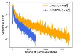
In the first experiment, we test the performances of DESTINY with different choices of stepsizes. Classical strategies for choosing stepsizes, such as line search, are not applicable in the decentralized setting. Recently, BB stepsizes have been introduced to the decentralized optimization for strongly convex problems [15]. In order to improve the performance of DESTINY, we intend to apply the following BB stepsizes.

\eta^{\mathrm{BB}}_{i,k}=\left\lvert\frac{\left\langle S_{i,k},J_{i,k}\right\rangle}{\left\langle J_{i,k},J_{i,k}\right\rangle}\right\rvert,

where $S_{i,k}=X_{i,k}-X_{i,k-1}$ , and $J_{i,k}=D_{i,k}-D_{i,k-1}$ . As illustrated in Figure 1, the above BB stepsizes can significantly enhance the efficiency of DESTINY. Hence, in subsequent experiments, we equip DESTINY with BB stepsizes by default. To the best of our knowledge, this is the first attempt, for nonconvex optimization problems, to accelerate the convergence of decentralized algorithms by BB stepsizes.

Refer to caption — (a) Substationarity Violation

Next, we present that our algorithm is not sensitive to the penalty parameter $\beta$ . Figure 2 depicts the performances of DESTINY with different values of $\beta$ which are distinguished by colors. In Figure 2(c), the y-axis depicts the feasibility violation in the logarithmic scale, which is defined by:

\sqrt{\dfrac{1}{d}\sum\limits_{i=1}^{d}\left\|X_{i,k}^{\top}X_{i,k}-I_{p}\right\|^{2}_{\mathrm{F}}}.

We can observe that the curves of substationarity violations, consensus errors, and feasibility violations almost coincide with each other, which indicates that DESTINY has almost the same performance in a wide range of penalty parameters. This observation validates the robustness of our algorithm to penalty parameters. Therefore, we fix $\beta=1$ by default in the subsequent experiments.

4.3 Comparison on decentralized PCA

In this subsection, we compare the performance of DESTINY in solving decentralized PCA problems (1.3) with some other state-of-the-art methods, including ADSA[12], DRGTA [5], and DeEPCA [47]. Among these three algorithms, ADSA and DRGTA require to choose the stepsize. In the empirical experiments, we find that DRGTA also benefits from the BB stepsizes, but ADSA can not converge with it. Hence, DRGTA is equipped with the same BB stepsizes as DESTINY, while the stepsize of ADSA is fixed as a hand-optimized constant. In the following experiments, for fair comparisons, both DRGTA and DeEPCA perform only one round of communications per iteration.

In order to assess the quality of the above four solvers, we perform a set of experiments on randomly generated matrices as described in Subsection 4.1. The network is built based on an Erdos-Renyi graph with $\mathtt{prob}$ ranging from $0.2$ to $0.6$ with increment $0.2$ . Other experimental settings are $n=300$ , $m=3200$ , $p=10$ , $\xi=0.95$ , and $d=32$ . The numerical results are illustrated in Figure 3. It can be observed that DeEPCA and DRGTA can not converge when $\mathtt{prob}=0.2$ , which signifies that a single consensus step per iteration is not sufficient for these two algorithms to converge in sparse networks. Apart from this special case, DeEPCA has the best performance among all the algorithms. Moreover, DESTINY is competitive with ADSA and significantly outperforms DRGTA in all cases. It should be noted that DeEPCA and ADSA are tailored for decentralized PCA problems and can not be extended to generic cases.

4.4 Comparison on decentralized OLSR

In this subsection, the abilities of DESTINY and DRGTA [5] are examined in solving decentralized OLSR problems (1.4) on the real-world text dataset Cora [25]. For our testing in this case, we select a subset of Cora and extract the first $n=100$ features to use, which contains research papers from three subfields, including data structure (DS), hardware and architecture (HA), and programming language (PL). The number of samples $(m)$ and classes $(p)$ are summarized as follows.

•

Cora-DS: $m=751$ , $p=9$ .
•

Cora-HA: $m=400$ , $p=7$ .
•

Cora-PL: $m=1575$ , $p=9$ .

The detailed descriptions and download links of this dataset can be found in [51]. The number of agents is set to $d=32$ in this experiment. We provide the numerical results in Figure 4, which demonstrates that DESTINY attains better performances than DRGTA in terms of both substationarity violations and consensus errors. Therefore, our algorithm manifests its efficiency in dealing with real-world datasets.

4.5 Comparison on decentralized SDL

In this subsection, we evaluate the performance on decentralized SDL problems (1.5) of DESTINY and DRGTA [5]. Three image datasets popular in machine learning research are tested in the following experiments, including MNIST¹¹1Available from http://yann.lecun.com/exdb/mnist/ , CIFAR-10²²2Available from https://www.cs.toronto.edu/~kriz/cifar.html , and CIFAR-100 ${}^{\ref{note:CIFAR}}$ . We summarize the numbers of features $(n)$ and samples $(m)$ as follows.

•

MNIST: $n=784$ , $m=60000$ .
•

CIFAR-10: $n=3072$ , $m=50000$ .
•

CIFAR-100: $n=3072$ , $m=50000$ .

For our testing, the numbers of computed bases and agents are set to $p=1$ and $d=32$ , respectively. Numerical results from this experiment are given in Figure 5. It can be observed that DESTINY always dominates DRGTA in terms of both substationarity violations and consensus errors. These results indicate that the observed superior performance of our algorithm is not just limited to PCA and OLSR problems.

5 Conclusions

As a powerful and fundamental tool, Riemannian optimization has been adapted to solving consensus problems on a multi-agent network, giving rise to the decentralized Riemannian gradient tracking algorithm (DRGTA) on the Stiefel manifold. In order to guarantee the convergence, DRGTA requires multiple rounds of communications per iteration, and hence, the communication overheads are very high. In this paper, we propose an infeasible decentralized algorithm, called DESTINY, which only invokes a single round of communications per iteration. DESTINY seeks a consensus in the Euclidean space directly by resorting to an elegant approximate augmented Lagrangian function. Even in the non-distributed setting, the proposed algorithm is still new for optimization problems over the Stiefel manifold.

Most existing works on analyzing the convergence of gradient tracking based algorithms impose stringent assumptions on objective functions, such as global Lipschitz smoothness and coerciveness. In our case of DESTINY which tackles decentralized optimization problems with nonconvex constraints, we are able to derive the global convergence and worst case complexity under rather mild conditions. The objective function is only assumed to be locally Lipschitz smooth.

Comprehensive numerical comparisons are carried out under the distributed setting with test results strongly in favor of DESTINY. Most notably, the rounds of communications required by DESTINY are significantly fewer than what are required by DRGTA.

Finally, some topics are worthy of future studies to fully understand the behavior and realize the potential of DESTINY and its variants. For example, the asynchronous version of DESTINY is worthy of investigating to address the load balance issues in the distributed environments. And more work is needed to adapt DESTINY to the dynamic network settings so that it can find a wider range of applications.

Acknowledgment

The authors would like to thank Prof. Lei-Hong Zhang for sharing the Cora dataset, and Prof. Qing Ling and Dr. Nachuan Xiao for their insightful discussions.

References

[1] T. E. Abrudan, J. Eriksson, and V. Koivunen, Steepest descent algorithms for optimization under unitary matrix constraint, IEEE Transactions on Signal Processing, 56 (2008), pp. 1134–1147.
[2] P.-A. Absil, C. G. Baker, and K. A. Gallivan, Trust-region methods on Riemannian manifolds, Foundations of Computational Mathematics, 7 (2006), pp. 303–330.
[3] P.-A. Absil, R. Mahony, and R. Sepulchre, Optimization algorithms on matrix manifolds, Princeton University Press, 2008.
[4] T.-H. Chang, M. Hong, and X. Wang, Multi-agent distributed optimization via inexact consensus ADMM, IEEE Transactions on Signal Processing, 63 (2015), pp. 482–497.
[5] S. Chen, A. Garcia, M. Hong, and S. Shahrampour, Decentralized Riemannian gradient descent on the Stiefel manifold, in Proceedings of the 38th International Conference on Machine Learning, vol. 139, PMLR, 2021, pp. 1594–1605.
[6] Y. Chen, K. Yuan, Y. Zhang, P. Pan, Y. Xu, and W. Yin, Accelerating gossip SGD with periodic global averaging, in Proceedings of the 38th International Conference on Machine Learning, vol. 139, PMLR, 2021, pp. 1791–1802.
[7] A. Daneshmand, G. Scutari, and V. Kungurtsev, Second-order guarantees of distributed gradient algorithms, SIAM Journal on Optimization, 30 (2020), pp. 3029–3068.
[8] P. Di Lorenzo and G. Scutari, Next: In-network nonconvex optimization, IEEE Transactions on Signal and Information Processing over Networks, 2 (2016), pp. 120–136.
[9] A. Edelman, T. A. Arias, and S. T. Smith, The geometry of algorithms with orthogonality constraints, SIAM Journal on Matrix Analysis and Applications, 20 (1998), pp. 303–353.
[10] A. Gang and W. U. Bajwa, FAST-PCA: A fast and exact algorithm for distributed principal component analysis, arXiv:2108.12373, (2021).
[11] A. Gang and W. U. Bajwa, A linearly convergent algorithm for distributed principal component analysis, Signal Processing, 193 (2022), p. 108408.
[12] A. Gang, H. Raja, and W. U. Bajwa, Fast and communication-efficient distributed PCA, in Proceedings of the 2019 International Conference on Acoustics, Speech and Signal Processing, IEEE, 2019, pp. 7450–7454.
[13] B. Gao, X. Liu, X. Chen, and Y.-X. Yuan, A new first-order algorithmic framework for optimization problems with orthogonality constraints, SIAM Journal on Optimization, 28 (2018), pp. 302–332.
[14] B. Gao, X. Liu, and Y.-X. Yuan, Parallelizable algorithms for optimization problems with orthogonality constraints, SIAM Journal on Scientific Computing, 41 (2019), pp. A1949–A1983.
[15] J. Gao, X.-W. Liu, Y.-H. Dai, Y. Huang, and P. Yang, Achieving geometric convergence for distributed optimization with Barzilai-Borwein step sizes, Science China Information Sciences, 65 (2022), pp. 1–2.
[16] D. Hajinezhad and M. Hong, Perturbed proximal primal–dual algorithm for nonconvex nonsmooth optimization, Mathematical Programming, 176 (2019), pp. 207–245.
[17] M. Hong, D. Hajinezhad, and M.-M. Zhao, Prox-PDA: The proximal primal-dual algorithm for fast distributed nonconvex optimization and learning over networks, in International Conference on Machine Learning, PMLR, 2017, pp. 1529–1538.
[18] J. Hu, B. Jiang, L. Lin, Z. Wen, and Y.-X. Yuan, Structured quasi-Newton methods for optimization with orthogonality constraints, SIAM Journal on Scientific Computing, 41 (2019), pp. A2239–A2269.
[19] J. Hu, A. Milzarek, Z. Wen, and Y. Yuan, Adaptive quadratically regularized Newton method for Riemannian optimization, SIAM Journal on Matrix Analysis and Applications, 39 (2018), pp. 1181–1207.
[20] B. Jiang and Y.-H. Dai, A framework of constraint preserving update schemes for optimization on Stiefel manifold, Mathematical Programming, 153 (2015), pp. 535–575.
[21] T. Krasulina, Method of stochastic approximation in the determination of the largest eigenvalue of the mathematical expectation of random matrices, Automatation and Remote Control, 2 (1970), pp. 50–56.
[22] Q. Ling, W. Shi, G. Wu, and A. Ribeiro, DLM: Decentralized linearized alternating direction method of multipliers, IEEE Transactions on Signal Processing, 63 (2015), pp. 4051–4064.
[23] Y. Liu, W. Xu, G. Wu, Z. Tian, and Q. Ling, Communication-censored ADMM for decentralized consensus optimization, IEEE Transactions on Signal Processing, 67 (2019), pp. 2565–2579.
[24] J. H. Manton, Optimization algorithms exploiting unitary constraints, IEEE Transactions on Signal Processing, 50 (2002), pp. 635–650.
[25] A. K. McCallum, K. Nigam, J. Rennie, and K. Seymore, Automating the construction of internet portals with machine learning, Information Retrieval, 3 (2000), pp. 127–163.
[26] A. Nedic, A. Olshevsky, and W. Shi, Achieving geometric convergence for distributed optimization over time-varying graphs, SIAM Journal on Optimization, 27 (2017), pp. 2597–2633.
[27] A. Nedic and A. Ozdaglar, Distributed subgradient methods for multi-agent optimization, IEEE Transactions on Automatic Control, 54 (2009), pp. 48–61.
[28] Y. Nishimori and S. Akaho, Learning algorithms utilizing quasi-geodesic flows on the Stiefel manifold, Neurocomputing, 67 (2005), pp. 106–135.
[29] S. U. Pillai, T. Suel, and S. Cha, The Perron-Frobenius theorem: some of its applications, IEEE Signal Processing Magazine, 22 (2005), pp. 62–75.
[30] G. Qu and N. Li, Harnessing smoothness to accelerate distributed optimization, IEEE Transactions on Control of Network Systems, 5 (2017), pp. 1245–1260.
[31] S. S. Ram, A. Nedić, and V. V. Veeravalli, Distributed stochastic subgradient projection algorithms for convex optimization, Journal of Optimization Theory and Applications, 147 (2010), pp. 516–545.
[32] T. D. Sanger, Optimal unsupervised learning in a single-layer linear feedforward neural network, Neural Networks, 2 (1989), pp. 459–473.
[33] H. Sato, A Dai–Yuan-type Riemannian conjugate gradient method with the weak Wolfe conditions, Computational Optimization and Applications, 64 (2016), pp. 101–118.
[34] I. D. Schizas and A. Aduroja, A distributed framework for dimensionality reduction and denoising, IEEE Transactions on Signal Processing, 63 (2015), pp. 6379–6394.
[35] G. Scutari and Y. Sun, Distributed nonconvex constrained optimization over time-varying digraphs, Mathematical Programming, 176 (2019), pp. 497–544.
[36] W. Shi, Q. Ling, G. Wu, and W. Yin, EXTRA: An exact first-order algorithm for decentralized consensus optimization, SIAM Journal on Optimization, 25 (2015), pp. 944–966.
[37] E. Stiefel, Richtungsfelder und fernparallelismus in n-dimensionalen mannigfaltigkeiten, Commentarii Mathematici Helvetici, 8 (1935), pp. 305–353.
[38] L. Wang, B. Gao, and X. Liu, Multipliers correction methods for optimization problems over the Stiefel manifold, CSIAM Transactions on Applied Mathematics, 2 (2021), pp. 508–531.
[39] L. Wang, X. Liu, and Y. Zhang, A distributed and secure algorithm for computing dominant SVD based on projection splitting, arXiv:2012.03461, (2020).
[40] , A communication-efficient and privacy-aware distributed algorithm for sparse PCA, arXiv:2106.03320, (2021).
[41] Z. Wen and W. Yin, A feasible method for optimization with orthogonality constraints, Mathematical Programming, 142 (2013), pp. 397–434.
[42] L. Xiao and S. Boyd, Fast linear iterations for distributed averaging, Systems & Control Letters, 53 (2004), pp. 65–78.
[43] N. Xiao and X. Liu, Solving optimization problems over the Stiefel manifold by smooth exact penalty function, arXiv:2110.08986, (2021).
[44] N. Xiao, X. Liu, and Y.-X. Yuan, A class of smooth exact penalty function methods for optimization problems with orthogonality constraints, Optimization Methods and Software, (2020), pp. 1–37.
[45] , A penalty-free infeasible approach for a class of nonsmooth optimization problems over the Stiefel manifold, arXiv:2103.03514, (2021).
[46] J. Xu, S. Zhu, Y. C. Soh, and L. Xie, Augmented distributed gradient methods for multi-agent optimization under uncoordinated constant stepsizes, in 54th IEEE Conference on Decision and Control, IEEE, 2015, pp. 2055–2060.
[47] H. Ye and T. Zhang, DeEPCA: Decentralized exact PCA with linear convergence rate, Journal of Machine Learning Research, 22 (2021), pp. 1–27.
[48] K. Yuan, Q. Ling, and W. Yin, On the convergence of decentralized gradient descent, SIAM Journal on Optimization, 26 (2016), pp. 1835–1854.
[49] J. Zeng and W. Yin, On nonconvex decentralized gradient descent, IEEE Transactions on Signal Processing, 66 (2018), pp. 2834–2848.
[50] Y. Zhai, Z. Yang, Z. Liao, J. Wright, and Y. Ma, Complete dictionary learning via $\ell_{4}$ -norm maximization over the orthogonal group, Journal of Machine Learning Research, 21 (2020), pp. 1–68.
[51] L.-H. Zhang, W. H. Yang, C. Shen, and J. Ying, An eigenvalue-based method for the unbalanced Procrustes problem, SIAM Journal on Matrix Analysis and Applications, 41 (2020), pp. 957–983.
[52] H. Zhao, Z. Wang, and F. Nie, Orthogonal least squares regression for feature extraction, Neurocomputing, 216 (2016), pp. 200–207.
[53] X. Zhu, A Riemannian conjugate gradient method for optimization on the Stiefel manifold, Computational Optimization and Applications, 67 (2017), pp. 73–110.

		$\displaystyle M_{g}=\sup\,\{\left\\|G_{i}(X)\right\\|_{\mathrm{F}}\mid X\in\mathcal{B},i\in[d]\};\quad M_{b}=\sup\,\{\left\\|\nabla b(X)\right\\|_{\mathrm{F}}\mid X\in\mathcal{B}\};$		(3.1)
		$\displaystyle L_{g}=\sup\,\left\{\dfrac{\left\\|G_{i}(X)-G_{i}(Y)\right\\|_{\mathrm{F}}}{\left\\|X-Y\right\\|_{\mathrm{F}}}\bigg{\|}X\neq Y,X\in\mathcal{B},Y\in\mathcal{B},i\in[d]\right\};$
		$\displaystyle L_{b}=\sup\,\left\{\dfrac{\left\\|\nabla b(X)-\nabla b(Y)\right\\|_{\mathrm{F}}}{\left\\|X-Y\right\\|_{\mathrm{F}}}\bigg{\|}X\neq Y,X\in\mathcal{B},Y\in\mathcal{B}\right\};\quad C_{1}=\dfrac{\lambda^{2}\left(1+\lambda^{2}\right)}{1-\lambda^{2}};$
		$\displaystyle L_{f}=\sup\,\left\{\dfrac{\left\\|\nabla f(X)-\nabla f(XX^{\top}X)\right\\|_{\mathrm{F}}}{\left\\|X\left(X^{\top}X-I_{p}\right)\right\\|_{\mathrm{F}}}\bigg{\|}X\neq XX^{\top}X,X\in\mathcal{B}\right\};\quad\gamma=\dfrac{1-\lambda^{2}}{2\lambda^{2}}.$

	$\displaystyle\left\\|\bar{X}_{k+1}^{\top}\bar{X}_{k+1}-I_{p}\right\\|_{\mathrm{F}}\leq{}$	$\displaystyle\left\\|\left(I_{n}-\eta\beta\bar{X}_{k}^{\top}\bar{X}_{k}\right)^{2}\left(\bar{X}_{k}^{\top}\bar{X}_{k}-I_{p}\right)\right\\|_{\mathrm{F}}+\eta^{2}\beta^{2}\left\\|\bar{X}_{k}^{\top}\bar{X}_{k}\left(\bar{X}_{k}^{\top}\bar{X}_{k}-I_{p}\right)\right\\|_{\mathrm{F}}$
		$\displaystyle+2\eta\left\\|\bar{X}_{k}^{\top}Y_{k}\right\\|_{\mathrm{F}}+2\eta^{2}\beta\left\\|\left(\bar{X}_{k}^{\top}\bar{X}_{k}-I_{p}\right)\bar{X}_{k}^{\top}Y_{k}\right\\|_{\mathrm{F}}+\eta^{2}\left\\|Y_{k}^{\top}Y_{k}\right\\|_{\mathrm{F}}$
	$\displaystyle\leq{}$	$\displaystyle\left(1-\dfrac{5}{6}\eta\beta\right)^{2}\left\\|\bar{X}_{k}^{\top}\bar{X}_{k}-I_{p}\right\\|_{\mathrm{F}}+\dfrac{49}{216}\eta^{2}\beta^{2}+\dfrac{7}{3}(1+M_{g})\eta$
		$\displaystyle+\dfrac{7}{18}(1+M_{g})\eta^{2}\beta+(1+M_{g})^{2}\eta^{2}$
	$\displaystyle\leq{}$	$\displaystyle\left(1-\dfrac{5}{6}\eta\beta\right)^{2}\left\\|\bar{X}_{k}^{\top}\bar{X}_{k}-I_{p}\right\\|_{\mathrm{F}}+\eta\left(4+3M_{g}\right)+\eta^{2}\left(1+M_{g}\right)^{2},$

	$\displaystyle\left\\|\bar{\mathbf{X}}_{k+1}-\mathbf{X}_{k+1}\right\\|_{\mathrm{F}}$	$\displaystyle=\left\\|\left(\mathbf{W}-\mathbf{J}\right)\left(\bar{\mathbf{X}}_{k}-\mathbf{X}_{k}\right)+\eta\left(\mathbf{W}-\mathbf{J}\right)\mathbf{D}_{k}\right\\|_{\mathrm{F}}$
		$\displaystyle\leq\left\\|\left(\mathbf{W}-\mathbf{J}\right)\left(\bar{\mathbf{X}}_{k}-\mathbf{X}_{k}\right)\right\\|_{\mathrm{F}}+\eta\left\\|\left(\mathbf{W}-\mathbf{J}\right)\mathbf{D}_{k}\right\\|_{\mathrm{F}}$
		$\displaystyle\leq\lambda\left\\|\bar{\mathbf{X}}_{k}-\mathbf{X}_{k}\right\\|_{\mathrm{F}}+\eta\lambda\left\\|\mathbf{D}_{k}\right\\|_{\mathrm{F}}$
		$\displaystyle\leq\lambda\left\\|\bar{\mathbf{X}}_{k}-\mathbf{X}_{k}\right\\|_{\mathrm{F}}+\eta\lambda C_{D},$

	$\displaystyle\left\\|\bar{\mathbf{D}}_{k+1}-\mathbf{D}_{k+1}\right\\|_{\mathrm{F}}$	$\displaystyle=\left\\|\left(\mathbf{W}-\mathbf{J}\right)\left(\bar{\mathbf{D}}_{k}-\mathbf{D}_{k}\right)-\left(I_{dn}-\mathbf{J}\right)\left(\mathbf{H}_{k+1}-\mathbf{H}_{k}\right)\right\\|_{\mathrm{F}}$
		$\displaystyle\leq\left\\|\left(\mathbf{W}-\mathbf{J}\right)\left(\bar{\mathbf{D}}_{k}-\mathbf{D}_{k}\right)\right\\|_{\mathrm{F}}+\left\\|\left(I_{dn}-\mathbf{J}\right)\left(\mathbf{H}_{k+1}-\mathbf{H}_{k}\right)\right\\|_{\mathrm{F}}$
		$\displaystyle\leq\lambda\left\\|\bar{\mathbf{D}}_{k}-\mathbf{D}_{k}\right\\|_{\mathrm{F}}+\left\\|\mathbf{H}_{k+1}-\mathbf{H}_{k}\right\\|_{\mathrm{F}}$
		$\displaystyle\leq\lambda\left\\|\bar{\mathbf{D}}_{k}-\mathbf{D}_{k}\right\\|_{\mathrm{F}}+3\sqrt{d},$

	$\displaystyle\left\\|\bar{\mathbf{X}}_{k+1}-\mathbf{X}_{k+1}\right\\|^{2}_{\mathrm{F}}=$	$\displaystyle\left\\|\left(\mathbf{W}-\mathbf{J}\right)\left(\bar{\mathbf{X}}_{k}-\mathbf{X}_{k}\right)-\eta\left(\mathbf{W}-\mathbf{J}\right)\left(\bar{\mathbf{D}}_{k}-\mathbf{D}_{k}\right)\right\\|^{2}_{\mathrm{F}}$
	$\displaystyle\leq$	$\displaystyle\left(1+\gamma\right)\left\\|\left(\mathbf{W}-\mathbf{J}\right)\left(\bar{\mathbf{X}}_{k}-\mathbf{X}_{k}\right)\right\\|^{2}_{\mathrm{F}}+\eta^{2}\left(1+1/\gamma\right)\left\\|\left(\mathbf{W}-\mathbf{J}\right)\left(\bar{\mathbf{D}}_{k}-\mathbf{D}_{k}\right)\right\\|^{2}_{\mathrm{F}}$
	$\displaystyle\leq$	$\displaystyle\lambda^{2}\left(1+\gamma\right)\left\\|\bar{\mathbf{X}}_{k}-\mathbf{X}_{k}\right\\|^{2}_{\mathrm{F}}+\eta^{2}\lambda^{2}\left(1+1/\gamma\right)\left\\|\bar{\mathbf{D}}_{k}-\mathbf{D}_{k}\right\\|^{2}_{\mathrm{F}},$

Decentralized Optimization Over the Stiefel Manifold by an Approximate Augmented Lagrangian Function

Abstract

1 Introduction

Assumption 1.

1.1 Broad applications

Application 1: Principal Component Analysis.

Application 2: Orthogonal Least Squares Regression.

Application 3: Sparse Dictionary Learning.

1.2 Literature survey

1.3 Contributions

1.4 Notations

1.5 Outline

2 Algorithm Development

2.1 Preliminaries

Definition 2.1.

Assumption 2.

2.2 Approximate augmented Lagrangian function

Lemma 2.2.

Proof.

2.3 Algorithm description

3 Convergence Analysis

Assumption 3.

3.1 Boundedness of iterates

Lemma 3.1.

Proof.

Case I: ‖X¯k⊤​X¯k−Ip‖F≤1/12\left\|\bar{X}_{k}^{\top}\bar{X}_{k}-I_{p}\right\|_{\mathrm{F}}\leq 1/12.

Case II: ‖X¯k⊤​X¯k−Ip‖F>1/12\left\|\bar{X}_{k}^{\top}\bar{X}_{k}-I_{p}\right\|_{\mathrm{F}}>1/12.

Proposition 3.2.

Proof.

3.2 Sufficient descent of the merit function

Lemma 3.3.

Proof.

Lemma 3.4.

Proof.

Lemma 3.5.

Proof.

Lemma 3.6.

Proof.

Proposition 3.7.

Proof.

3.3 Global convergence

Theorem 3.8.

Proof.

4 Numerical Simulations

4.1 Test problems

4.2 Default settings

4.3 Comparison on decentralized PCA

4.4 Comparison on decentralized OLSR

4.5 Comparison on decentralized SDL

5 Conclusions

Acknowledgment

References

Case I: $\left\|\bar{X}_{k}^{\top}\bar{X}_{k}-I_{p}\right\|_{\mathrm{F}}\leq 1/12$ .

Case II: $\left\|\bar{X}_{k}^{\top}\bar{X}_{k}-I_{p}\right\|_{\mathrm{F}}>1/12$ .