Decentralized Intermittent Feedback Adaptive Control of Non-triangular Nonlinear Time-varying Systems
Abstract
This paper investigates the decentralized stabilization problem for a class of interconnected systems in the presence of non-triangular structural uncertainties and time-varying parameters, where each subsystem exchanges information only with its neighbors and only intermittent (rather than continuous) states and input are to be utilized. Thus far to our best knowledge, no solution exists priori to this work, despite its high prevalence in practice. Two globally decentralized adaptive control schemes are presented based on the backstepping technique, the first one is developed in a continuous fashion by combining the philosophy of the modified congelation of variables based approach with the special treatment of non-triangular structural uncertainties, which avoids the derivative of time-varying parameters and eliminates the limitation of the triangular condition, thus largely broadens the scope of application. By making use of the important property that the partial derivatives of the constructed virtual controllers in each subsystem are all constant, the second scheme is developed through directly replacing the states in the preceding scheme with the triggered ones. Consequently, the non-differentiability of the virtual control stemming from intermittent state feedback is completely obviated. The internal signals under both schemes are rigorously shown to be globally uniformly bounded with the aid of several novel lemmas, while the stabilization performance can be enhanced by appropriately adjusting design parameters. Moreover, the inter-event intervals are ensured to be lower-bounded by a positive constant. Finally, numerical simulation verifies the benefits and efficiency of the proposed method.
Decentralized adaptive control, backstepping, event-triggering, non-triangular uncertain systems. \IEEEpeerreviewmaketitle
1 Introduction
Large-scale uncertain complex interconnected systems are frequently encountered [1, 2, 3, 4], decentralized adaptive control of such systems is currently facilitated by recent technological advances on computing and communication resources, which serves as an efficient and practical strategy to be employed for many reasons, such as simplicity of controller design and implementation. Communication network is necessary for signal transmission in large-scale nonlinear control systems owing to networked control systems (NCSs) with advantages of lower cost, easier maintenance and higher reliability [5]. However, there is a gap between the decentralized control and the network under such framework, because the sensor data cannot be transmitted/updated in real time on account of limited communication bandwidth and channels, which potentially degrades the control performance of large-scale nonlinear system.
To preserve a trade-off between communication resource usage and control performance, the emergence of event-triggered control is stimulated as an appealing method for saving energy and communication resources, which enables communication only when certain predefined condition is triggered (see e.g., [6, 7] and the references therein). Early available results on event-triggered control mainly focus on linear systems, see [8, 9] for examples. An extension work to nonlinear systems is pioneered in [10], yet the closed-loop dynamic should be input-to-state stable (ISS). Such limitation is removed in [11] by codesigning an event-triggered control algorithm. However, the system models considered in [10, 11] are required to be exactly known. To handle the uncertainties for nonlinear systems, some event-triggered adaptive control schemes are advocated via the backstepping design procedure, see e.g. [12, 13] and the references therein. Nonetheless, those results are dedicated to the case where only the control input is intermittently transmitted over the network while continuous feedback of plant states are required, thus merely saving the communication resources in the controller-to-actuator channel, but not applicable for the senor-to-controller ones.
For the past few years, control design via intermittent state feedback has stirred an increasing amount of attention in the literature due to its more efficient usage of available limited resources. In this direction, two types of strategies should be highlighted. The first one is the state-triggered control using intermittent output only. In this direction, a state-triggered output feedback control scheme is proposed in [14] for delta operator systems with matched uncertainties. In [15], the problem of decentralized adaptive backstepping based output feedback control is addressed for a class of nonlinear interconnected systems. However, in both solutions, the alleviation on communication burden is still limited because only the output is triggered. The second one is the state-triggered control via intermittent full-state feedback. For this scenario, some efforts have been made in [16, 17] by using backstepping based adaptive control, wherein the models are in low-order form [16] or in normal form [17]. More recently, with the aid of dynamic surface control (DSC) technique, such restriction is explicitly relaxed in [18] for a family of nonlinear systems with constant parametric uncertainties. The idea of designing a distributed state-triggered control algorithm for networked nonlinear system with mismatched and nonparametric uncertainties is further introduced in [19]. The result of [20] solves the problem of stabilizing large-scale interconnected systems by distributed state-triggered controllers built on the ISS condition. Nevertheless, the approaches in [18, 19, 20] are tailored for nonlinear systems in triangular form. Meanwhile, the plant parameters involved in the above results are all restricted to constants. In most applications, however, plant parameters may vary with time rapidly [21]. For instance, traffic free speed is considered as a time-varying parameter in freeway traffic systems control, since changes in weather, air pressure, etc., can strongly influences free speed; in automatic train control problems, the mass of the train load that affects the resistance imposed on the train, may not be the same at different runs. Therefore it is vitally important to relax or even remove these strong restrictions, and broaden the applicability of the backstepping-based state-triggered stability theory to cover system models in non-triangular forms with time-varying parameters.
Motivated by the aforementioned discussion, in this work we develop a decentralized event-triggered adaptive backstepping control method for nonlinear interconnected systems with non-triangular structural uncertainties and unknown time-varying parameters. Under such setting it is actually nontrivial to achieve this goal, this is because two major technical difficulties are present in control design and stability analysis. First, the models of subsystems are all in non-trival non-triangular form with coupling interactions and unknown time-varying parameters that directly challenges the traditional back-stepping design procedure, a tailored technique for triangular systems with constant parameters; Second, with intermittent feedback signals arising from event-triggering, the underlying problem becomes even more complicated when carrying out backstepping design because the repetitive differentiation of virtual control signals (with respect to the triggering signals) is no longer feasible (literally undefined due to the nature of the event-triggering). In this work, we propose two globally decentralized adaptive backstepping control design approaches respectively for the cases with and without event-triggering setting. The first one is developed in a continuous fashion that successfully removes the triangular-form-limitation imposed on the system model by properly treating the non-triangular structural uncertainties for the backstepping design, and simultaneously restrains the affects of the parameter-induced perturbation by freezing the time-varying parameters at the centers, thus avoiding the derivative of time-varying parameters and further relaxing the related state-of-the art conditions [22, 23]. It is shown that the partial derivatives of virtual controllers in each subsystem with respect to states are constants. With such property, the second control scheme is then constructed by replacing the states in the first one with the triggering states, thus circumventing the aforementioned non-differentiability in a global manner. Several lemmas are established to facilitate the authentication of the global uniform boundedness of all the closed-loop signals in both strategies with the stabilization performance improvable by appropriately adjusting design parameters. Moreover, a strictly positive lower bound on the inter transmission times is enforced by the proposed event triggering mechanism (ETM), thus the notorious Zeno phenomenon is avoided. To our best knowledge, this is the first adaptive backstepping control solution for interconnected nonlinear systems under event-triggering setting that is able to tolerate non-triangular structural uncertainties and unknown time-varying parameters.
2 Problem Formulation
Consider the following nonlinear system consists of interconnected subsystems, with the th subsystem modeled as:
| (1) |
for , where , is the system state, with , and are the control input and output, respectively, and are known functions, with , is the unknown parameter vector, denotes the nonlinear coupling interaction from the th subsystem for , and the modeling error of the th subsystem for 111Arguments of some functions will be omitted hereafter if no confusion is likely to occur..
The objective of this paper is to develop the globally decentralized adaptive backstepping control scheme for system (1) using only locally intermittent feedback signals, such that
-
The global uniform boundedness of the closed-loop signals is ensured, while all the subsystem outputs are steered into an assignable residual set around zero;
-
The Zeno behavior is precluded.
To move on, we make the following assumptions.
Assumption 1 [24]. The unknown nonlinear function satisfies the following condition:
| (2) |
for , , where is the unknown coupling gain, which denotes the magnitudes or strengths of the modeling errors and coupling interactions, and is an unknown constant.
Assumption 2. The parameter is piecewise continuous and , for all , where is an unknown compact set. The “radius” of , denoted by , is assumed to be bounded but not necessarily known.
Assumption 3. The functions and satisfy the global Lipschitz continuity condition such that
| (3) | ||||
| (4) |
where and are unknown bounded constants.
Remark 1. Notice from (2) that is bounded by a function that allows dependence on all subsystems states, in other words, the uncertainties under consideration fails to satisfy the triangular structure. In addition, it holds that the larger the value of is, the stronger the influence degree would be. Such interactions are rather general in numerous real-world systems, such as power systems, water systems, traffic systems and flexible space structures [25, 26], which tend to degrade the system performance and thus challenge the reliability and safety of the system.
Remark 2. Assumption 1 can be commonly found in literature, for example, [24, 27]. As noted in Assumption 2, only the “radius” of , i.e., is assumed to be bounded, which is more general than the existing results [28, 29]. Specifically, it is assumed that with for all in [28], where is a known continuous function and is a known positive constant. Besides, considered in [29] is required to be available for the control design. Assumption 3 is quite common, see [15, 18] for examples.
3 Decentralized Continuous Adaptive Backstepping Control
In this section, a decentralized adaptive backstepping control scheme is developed using locally continuous state signals, which can also be regarded as the basis of the control scheme via intermittent state feedback in next section. To this end, we first carry out the following change of coordinates:
| (5) | ||||
| (6) |
The decentralized adaptive backstepping control scheme under continuous state feedback is designed as:
| (7) | ||||
| (8) | ||||
| (9) |
where , and , are positive design parameters, is the partial derivative of to , which is a constant that relies on , and . The updating law of is designed as:
| (10) |
where is some positive design parameter, is the estimate of , with , and is a positive definite design matrix.
At this stage, the following lemma is introduced.
Lemma 1. [24] The state vector and its transformation vector obey the following relationship, with :
| (11) |
Proof. See Appendix A.
Now we are ready to state the following theorem.
Theorem 1. Consider the interconnected nonlinear non-triangular system (1) under Assumptions 1-3, if using the decentralized adaptive controller (9), with the adaptive law (10), then it holds that: i) the global uniform boundedness of the closed-loop signals is ensured; and ii) all the subsystem outputs are steered into a residual set around zero, and the stabilization performance can be improved with some proper choices of the design parameters.
Proof. The proof is composed of the following steps.
Step 1: Consider the Lyapunov function . From (1), (5) and (6), the derivative of is computed as
| (12) |
According to Assumption 1, it is derived that
| (13) | ||||
| (14) |
By utilizing (7), (13) and (14), is expressed as
| (15) |
Step : Consider the Lyapunov function . Using (1) and (6), is derived as
| (16) |
Based on Assumption 1 and using Young’s inequality, it is seen that
| (17) | ||||
| (18) |
| (19) | ||||
| (20) |
By using (8), (15), (17)-(20), it can be derived from (16) that
| (21) |
Step : Consider the following Lyapunov function:
| (22) |
where is an unknown bounded constant vector. Different from the related control designs [12, 16, 17], here we construct the adaptive parameter term , instead of , which is one of the key steps to avoid the appearance of , while ensuring system stability simultaneously, as detailed in the sequel. From (1), (6), (9), (22) and using Young’s inequality, is evaluated as
| (23) |
Substituting (10) into (23) yields
| (24) |
where . In accordance with Lemma 1 and Assumptions 1-2, it can be obtained that
| (25) |
Here, we pause to stress that, the effect of the parameter-induced perturbation term is handled in a non-compensatory manner due to the involvement of ETM, rather than making compensation for it as proposed in [29], see Remark 7 for more details. By using (25), then can be further bounded as
| (26) |
Consider the Lyapunov function , we can obtain
| (27) |
where . By applying Lemma 1, it can be derived from (27) that
| (28) |
where by choosing , i.e., larger enough, , and . Then it holds that , with .
Now we are ready to prove in detail that the results i) and ii) in Theorem 1 are ensured.
Stability Analysis. From the above analysis, we have , it follows that and are bounded, . From (5), (6), (7) and (8), it is established that is bounded, . Then it can be derived from (9) that is bounded. Therefore, all signals in the closed-loop system are globally uniformly bounded.
Performance Analysis. As , we have , which implies that is ensured to attenuate to a residual set around zero. In addition, from the definition of , and , it holds that the upper bound of can be decreased by increasing design parameters and , or decreasing design parameter and , .
Remark 3. The non-triangular structural uncertainties involve both modeling errors and nonlinear coupling interactions, thus are difficult to tackle. For the first part, by constructing a nonlinear compensation term in the virtual controllers of each subsystem , as seen in (8), we naturally offset the terms related to in (18) and (20). Whereas the uncertainties in the second part contain nonlinear coupling interactions among subsystems, it is even more challenging to handle. Here, inspired by the ideas in [24], we first keep all terms associated with in each recursive step, and then cope with them in the final step with the aid of Lemma 1. It is worth noting that what is considered here is an entirely different and more difficult implementation scenario than the one in [24], where the traditional backstepping method can be directly used in [24] as state/input-triggering is not considered. Meanwhile the work in [24] involves only constant parametric uncertainties which therefore can be easily handled by using adaptive parameter estimates methods.
4 Decentralized Event-triggered Adaptive Backstepping Control
In this section, a decentralized adaptive backstepping control scheme under event-triggering setting is constructed upon the previous scheme, with feasibility and stability analysis provided. Such strategy not only inherits the ability of handling non-triangular structural uncertainties and time-varying parameters in the continuous scheme, but also evades the non-differentiability issue.
4.1 Event Triggering Mechanism
Inspired by the ETM presented in [12, 16], we denote , and , , as the local states information, other subsystem states information and the actuation signal information, respectively, which broadcast their information according to the devised ETM. Since , and denote the th event time for system , other subsystem and actuation signal broadcasting theirs information, respectively, which indicates that , and remain unchanged as
| (29) |
for . Now we propose the following triggering conditions that only depends on locally available information:
| (30) | ||||
| (31) | ||||
| (32) |
where , and are positive triggering thresholds, , and denote the first instants when (30)-(32) are fulfilled, respectively.
Remark 4. The designed ETM allows all the states sensoring and data transmission to be executed intermittently on the event-driven basis, and the states include those from the subsystem itself and its neighbors (not just the states between subsystems), thus different from that in [16, 17], which implies that the sensors do not need to be powered all the time and the data from the sensors to the controllers does not have to be transmitted ceaselessly. Besides, the communication between the control unit and the system can be made less frequently. In such a way, the proposed approach is more efficient in terms of saving communication and energy resources (despite the systems under consideration are more general interconnected nonlinear non-triangular forms) in comparison to the existing ones [12, 13, 16, 17], therein either states or control input are transmitted intermittently over the network.
4.2 Controller Design
Since only locally intermittent state signals (rather than its continuous value) are available in controlling the system in case of event-triggering, we modify the coordinate transformation defined in (5)-(6) into the following form by replacing with :
| (33) | ||||
| (34) |
Based upon intermittent state feedback, the decentralized event-triggered adaptive backstepping control scheme is constructed as:
| (35) | ||||
| (36) | ||||
| (37) |
where , and , are positive design parameters. The updating laws of is designed as:
| (38) |
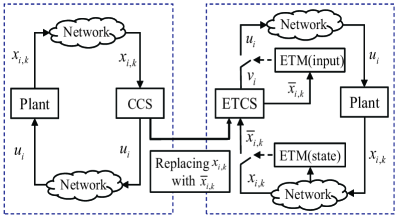
where is a positive design parameter and is a positive definite design matrix. The proposed two globally decentralized adaptive backstepping control strategies and their relationship are conceptually shown in Fig. 1.
To ensure the global uniform boundedness of all the closed-loop signals, we establish the following lemma.
Lemma 2. The effects of event-triggering are bounded as follows:
| (39) | ||||
| (40) |
for , , where and are positive constants that depend on the triggering thresholds , and , and the design parameters , and .
Proof. See Appendix B.
Remark 5. Thanks to the proposed modified congelation of variables based approach and a special treatment on non-triangular uncertainties, the partial derivatives in each subsystem are all ensured to be constant. Such property ensures that the impacts of event-triggering are bounded by constants, as detailed in Lemma 2. It is not trivial to derive such property, especially in the presence of serious uncertainties and time-varying parameters. Specifically, in the available adaptive state-triggered results such as [17, 18, 19], only systems in norm form exhibit this property [17]; in the nonlinear strict-feedback systems with parametric/non-parametric uncertainties [18, 19], one can only prove that the triggering errors are bounded by some time-varying functions, while requiring the exploitation of DSC techniques or neural networks (NN) based approximators (which can only obtain a semi-global result). Therefore it is even more challenging to retain such property for the non-triangular nonlinear time-varying interconnected systems actually considered here.
We are in the position to state the following theorem.
Theorem 2. Consider the interconnected nonlinear non-triangular system (1) under Assumptions 1-3, if using the decentralized adaptive controller (37), with adaptive law (38) and triggering conditions (30)-(32), it then holds that: i) the global uniform boundedness of the closed-loop signals is ensured; ii) all the subsystem outputs are steered into a residual set around zero, yet the stabilization performance can be improved with some proper choices of the design parameters; and iii) the Zeno phenomenon is precluded.
Proof. The proof of the claims in the theorem consists of two parts: stability analysis and exclusion of Zeno behavior.
1) Stability analysis. This part consists of the following steps.
Step 1:
Consider a Lyapunov function . From (1), (5), (6) and (7), the derivative of is expressed as
| (41) |
Step : Consider . By using (1), (6), (8) and (41), we can deduce that
| (42) |
Step : Consider the Lyapunov function , where is defined as before. Note that the control law in (37) can be rewritten as
| (43) |
From (1), (6), (42) and (43), is expressed as
| (44) |
Substituting (38) into (44), it follows that
| (45) |
where . Furthermore, becomes
| (46) |
with
| (47) |
According to Assumption 3, we can obtain that
| (48) | ||||
| (49) |
Notice from (47), (48), (49) and invoking Lemma 1, it holds that
| (50) |
where , , , , and . In accordance with (25), (46) and (50), the following inequality holds
| (51) |
where . Consider the Lyapunov function . With (51) in mind, we have
| (52) |
where , and by choosing , i.e., and larger enough, and . Thus we can obtain that , with .
In what follows, we show that results i)-iii) in Theorem 2 are ensured. By following the similar lines as the proof of Theorem 1, the results i)-ii) can be drawn. Next, we show that the result iii) is ensured. Define , , then it holds that
| (53) |
As remains unchanged for , one has and . Since , , , and , are all bounded, it is derived that there exists positive constant , such that , which implies that . Similarly, it holds that and , where , and are positive constants. Therefore the Zeno behavior is excluded.
Remark 6. To overcome the non-differentiability issue, we first develop a decentralized adaptive backstepping control scheme (7)-(10) in a continuous fashion by properly treating the non-triangular structural uncertainties for the backstepping design, and simultaneously restrains the affects of the parameter-induced perturbation via freezing the time-varying parameters at the centers. Afterwards, based upon the preceding scheme a decentralized adaptive event-triggered backstepping control scheme (35)-(38) is proposed by replacing the states in the preceding scheme with , in which one key property utilized is that the partial derivatives in each subsystem are all ensured to be constant. Finally, the crucial lemmas 1-2 are elaborately deduced with rigorous proofs for establishing stability condition under such replacement.
Remark 7. For handling the influence of the perturbation term resulted from time-varying parameters, an alternative is the compensation approach adopted in [29], which, however, is no longer applicable in this work. If a similar treatment is adopted, a compensation term will be added to the controller , and thus the adverse effect term caused by triggering error appears, which undoubtedly poses great difficulties in the stability analysis. To circumvent this problem, we handle such term in a non-compensatory manner with the aid of Lemma 1, as shown in (25), from which we obtain that the upper bound of relies on only, thereby can be incorporated into the negative term in (52).
Remark 8. Compared with existing results for time-varying systems [22, 23], where the adverse effects induced by time-varying parameters are directly addressed, this work obviously exhibits its merit because in accommodating the impact of the time-varying parameters, the somewhat restrictive conditions, such as the initial excitation [22], or the matched uncertainties [23], are completely removed. In addition, the existing methods related to event-triggered adaptive control [30, 31], although based upon non-triangular systems, are inapplicable to the setting of this work that is more comprehensive (i.e., both state and input are triggered) yet involves time-varying parameters. Moreover, the limitation of the triangular condition as typically imposed in current related works [18, 19, 20] is eliminated in this work, substantially broadening its scope of applications.
5 Simulation Verification
To verify the efficiency of the proposed control method, we consider the following interconnected system with two subsystems:
| (54) |
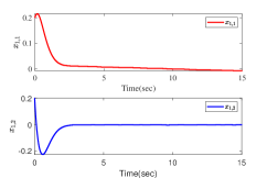
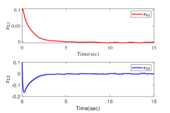
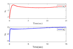
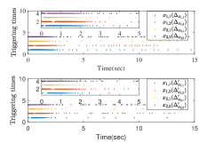
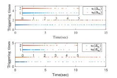
for . In the simulation, we set the initial states , , , , the design parameters , , , , , , , , , for , the time-varying parameters , , , , the nonlinear functions , , , , , , , , which do not meet the triangular structure requirements. From the given in (44), we set and . In addition, to test the effect of triggering thresholds on the tracking performance, we set the triggering thresholds as: 1) , , , , , ; 2) , , , , , , and the same set of other design parameters are used.
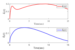
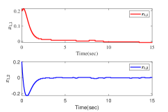
The results are presented in Fig. 2. Fig. 2 (a)-(b) show the state trajectories and , respectively. Fig. 2 (c) gives the control input . Fig. 2 (d) shows the time-varying adaptive estimated parameter vector . Fig. 2 (e)-(f) gives state trajectories and for the case of increasing triggering thresholds, respectively. The triggered times of and for different triggering thresholds are presented in Fig. 2 (g)-(h). From the simulation results, it can be concluded that all signals in the closed-loop systems are globally uniformly bounded, meanwhile all the subsystem outputs are steered into a residual set around zero. Besides, it holds that the larger the triggering thresholds, the smaller the triggering times. Nevertheless, it can be observed that the system performance is degraded to some extent.

6 Conclusion
This work presents a decentralized adaptive backstepping control scheme for non-triangular nonlinear time-varying systems via intermittent state feedback. The major technical challenge in developing such control strategy is to obviate the non-differentiability of the virtual control arising from intermittent state feedback, while coping with the non-triangular structural uncertainties and unknown time-varying parameters. By using the results established in the lemmas with rigorous proofs, it is shown that the closed-loop signal is globally uniformly bounded without Zeno behavior, and at the same time all the subsystem outputs are steered into an assignable residual set around zero. An interesting topic for future research is the consideration of the tracking control problem for such system.
7
8
References
- [1] P. Ioannou, “Decentralized adaptive control of interconnected systems,” IEEE Transactions on Automatic Control, vol. 31, no. 4, pp. 291–298, 1986.
- [2] J. Harmand and D. Dochain, “The optimal design of two interconnected (bio) chemical reactors revisited,” Computers & chemical engineering, vol. 30, no. 1, pp. 70–82, 2005.
- [3] C. Wen and D. J. Hill, “Global boundedness of discrete-time adaptive control just using estimator projection,” Automatica, vol. 28, no. 6, pp. 1143–1157, 1992.
- [4] Z.-P. Jiang, “Decentralized and adaptive nonlinear tracking of large-scale systems via output feedback,” IEEE Transactions on Automatic control, vol. 45, no. 11, pp. 2122–2128, 2000.
- [5] P. Antsaklis and J. Baillieul, “Special issue on technology of networked control systems,” Proceedings of the IEEE, vol. 95, no. 1, pp. 5–8, 2007.
- [6] W. H. Heemels, M. Donkers, and A. R. Teel, “Periodic event-triggered control for linear systems,” IEEE Transactions on automatic control, vol. 58, no. 4, pp. 847–861, 2012.
- [7] K. J. Aström, “Event based control,” in Analysis and design of nonlinear control systems. Springer, 2008, pp. 127–147.
- [8] A. Seuret, C. Prieur, S. Tarbouriech, and L. Zaccarian, “Lq-based event-triggered controller co-design for saturated linear systems,” Automatica, vol. 74, pp. 47–54, 2016.
- [9] W. Zhu, Z.-P. Jiang, and G. Feng, “Event-based consensus of multi-agent systems with general linear models,” Automatica, vol. 50, no. 2, pp. 552–558, 2014.
- [10] P. Tabuada, “Event-triggered real-time scheduling of stabilizing control tasks,” IEEE Transactions on Automatic Control, vol. 52, no. 9, pp. 1680–1685, 2007.
- [11] A. Adaldo, F. Alderisio, D. Liuzza, G. Shi, D. V. Dimarogonas, M. Di Bernardo, and K. H. Johansson, “Event-triggered pinning control of switching networks,” IEEE Transactions on Control of Network Systems, vol. 2, no. 2, pp. 204–213, 2015.
- [12] L. Xing, C. Wen, Z. Liu, H. Su, and J. Cai, “Event-triggered adaptive control for a class of uncertain nonlinear systems,” IEEE transactions on automatic control, vol. 62, no. 4, pp. 2071–2076, 2016.
- [13] M. Ghodrat and H. J. Marquez, “On the local input–output stability of event-triggered control systems,” IEEE Transactions on Automatic Control, vol. 64, no. 1, pp. 174–189, 2018.
- [14] M. Abdelrahim, R. Postoyan, J. Daafouz, and D. Nešić, “Robust event-triggered output feedback controllers for nonlinear systems,” Automatica, vol. 75, pp. 96–108, 2017.
- [15] Z. Zhang, C. Wen, K. Zhao, and Y. Song, “Decentralized adaptive control of uncertain interconnected systems with triggering state signals,” Automatica, vol. 141, p. 110283, 2022.
- [16] W. Wang, C. Wen, J. Huang, and J. Zhou, “Adaptive consensus of uncertain nonlinear systems with event triggered communication and intermittent actuator faults,” Automatica, vol. 111, p. 108667, 2020.
- [17] W. Wang, J. Long, J. Zhou, J. Huang, and C. Wen, “Adaptive backstepping based consensus tracking of uncertain nonlinear systems with event-triggered communication,” Automatica, vol. 133, p. 109841, 2021.
- [18] Z. Zhang, C. Wen, L. Xing, and Y. Song, “Adaptive event-triggered control of uncertain nonlinear systems using intermittent output only,” IEEE Transactions on Automatic Control, 2021.
- [19] L. Sun, X. Huang, and Y. Song, “Distributed event-triggered control of networked strict-feedback systems via intermittent state feedback,” IEEE Transactions on Automatic Control, Review, 2022.
- [20] C. De Persis, R. Sailer, and F. Wirth, “Parsimonious event-triggered distributed control: A zeno free approach,” Automatica, vol. 49, no. 7, pp. 2116–2124, 2013.
- [21] Y. Zhang, B. Fidan, and P. A. Ioannou, “Backstepping control of linear time-varying systems with known and unknown parameters,” IEEE Transactions on Automatic Control, vol. 48, no. 11, pp. 1908–1925, 2003.
- [22] R. Goel and S. B. Roy, “Composite adaptive control for time-varying systems with dual adaptation,” arXiv preprint arXiv:2206.01700, 2022.
- [23] M. Arefi and M. Jahed-Motlagh, “Adaptive robust synchronization of rossler systems in the presence of unknown matched time-varying parameters,” Communications in Nonlinear Science and Numerical Simulation, vol. 15, no. 12, pp. 4149–4157, 2010.
- [24] J. Cai, C. Wen, L. Xing, and Q. Yan, “Decentralized backstepping control for interconnected systems with non-triangular structural uncertainties,” IEEE Transactions on Automatic Control, 2022.
- [25] Y. Zhou, D. Li, Y. Xi, and F. Gao, “Event-triggered distributed robust model predictive control for a class of nonlinear interconnected systems,” Automatica, vol. 136, p. 110039, 2022.
- [26] P. R. Pagilla, N. B. Siraskar, and R. V. Dwivedula, “Decentralized control of web processing lines,” IEEE Transactions on control systems technology, vol. 15, no. 1, pp. 106–117, 2006.
- [27] J. Cai, C. Wen, H. Su, Z. Liu, and L. Xing, “Adaptive backstepping control for a class of nonlinear systems with non-triangular structural uncertainties,” IEEE Transactions on Automatic Control, vol. 62, no. 10, pp. 5220–5226, 2016.
- [28] H. Ríos, D. Efimov, J. A. Moreno, W. Perruquetti, and J. G. Rueda-Escobedo, “Time-varying parameter identification algorithms: Finite and fixed-time convergence,” IEEE Transactions on Automatic Control, vol. 62, no. 7, pp. 3671–3678, 2017.
- [29] K. Chen and A. Astolfi, “Adaptive control for systems with time-varying parameters,” IEEE Transactions on Automatic Control, vol. 66, no. 5, pp. 1986–2001, 2020.
- [30] Y. Yao, J. Tan, J. Wu, and X. Zhang, “Event-triggered fixed-time adaptive neural dynamic surface control for stochastic non-triangular structure nonlinear systems,” Information Sciences, vol. 569, pp. 527–543, 2021.
- [31] ——, “Event-triggered fixed-time adaptive neural tracking control for stochastic non-triangular structure nonlinear systems,” Neural Computing and Applications, vol. 33, no. 22, pp. 15 887–15 899, 2021.