Decentralized Federated Learning with Model Caching on Mobile Agents
Abstract
Federated Learning (FL) aims to train a shared model using data and computation power on distributed agents coordinated by a central server. Decentralized FL (DFL) utilizes local model exchange and aggregation between agents to reduce the communication and computation overheads on the central server. However, when agents are mobile, the communication opportunity between agents can be sporadic, largely hindering the convergence and accuracy of DFL. In this paper, we study delay-tolerant model spreading and aggregation enabled by model caching on mobile agents. Each agent stores not only its own model, but also models of agents encountered in the recent past. When two agents meet, they exchange their own models as well as the cached models. Local model aggregation works on all models in the cache. We theoretically analyze the convergence of DFL with cached models, explicitly taking into account the model staleness introduced by caching. We design and compare different model caching algorithms for different DFL and mobility scenarios. We conduct detailed case studies in a vehicular network to systematically investigate the interplay between agent mobility, cache staleness, and model convergence. In our experiments, cached DFL converges quickly, and significantly outperforms DFL without caching.
1 Introduction
1.1 Federated Learning on Mobile Agents
Federated learning (FL) is a type of distributed machine learning (ML) that prioritizes data privacy [mcmahan2017communication]. The traditional FL involves a central server that connects with a large number of agents. The agents retain their data and do not share them with the server. During each communication round, the server sends the current global model to the agents, and a small subset of agents are chosen to update the global model by running stochastic gradient descent (SGD) [robbins1951stochastic] for multiple iterations on their local data. The central server then aggregates the updated parameters to obtain the new global model. FL is a natural fit for the emerging Internet-of-Things (IoT) systems, where each IoT device not only can sense its surrounding environment to collect local data, but also is equipped with computation resources for local model training, as well as communication interfaces to interact with a central server for model aggregation. Many IoT devices are mobile, ranging from mobile phones/tablets, autonomous cars/drones, to self-navigating robots, etc. In the recent research efforts on smart connected vehicles, there has been a focus on integrating vehicle-to-everything (V2X) networks with Machine Learning (ML) tools and distributed decision making [barbieri2022decentralized], particularly in the area of computer vision tasks such as traffic light and signal recognition, road condition sensing, intelligent obstacle avoidance, and intelligent road routing, etc. With FL, vehicles locally train deep ML models and upload only the model parameters (i.e., neural network weights and biases) to the central server. This approach not only reduces bandwidth consumption, as the size of model parameters is much smaller than the size of raw image/video data, but also leverages computing power on vehicles, and protects user privacy.
However, FL on mobile agents still faces communication and computation challenges. The movements of mobile agents, especially at high speed, lead to fast-changing channel conditions on the wireless connections between mobile agents and the central FL server, resulting in long latency in FL [niknam2020federated]. Battery-powered mobile agents also have limited power budget for long-range wireless communications. Meanwhile, the non-i.i.d data distributions on mobile agents make it difficult for local models to converge. As a result, FL on mobile agents to obtain an optimal global model remains an open challenge. Decentralized federated learning (DFL) has emerged as a potential solution where local model aggregations are conducted between neighboring mobile agents using local device-to-device (D2D) communications with high bandwidth, low latency and low power consumption [10251949] . Preliminary studies have demonstrated that decentralized FL algorithms have the potential to significantly reduce the high communication costs associated with centralized FL. However, blindly applying model aggregation algorithms, such as FedSDG [shokri2015privacy] and FedAvg [mcmahan2017communication], developed for centralized FL to distributed FL cannot achieve fast convergence and high model accuracy [liu2022distributed].
1.2 Delay-Tolerant Model Communication and Aggregation Through Caching
D2D model communication between a pair of mobile agents is possible only if they are within each other’s transmission ranges. If mobile agents only meet with each others sporadically, there will not be enough model aggregation opportunity for fast convergence. In addition, with non-i.i.d data distributions on agents, if an agent only meets with agents from a small cluster, there is no way for the agent to interact with models trained by data samples outside of its cluster, leading to disaggregated local models that cannot perform well on the global data distribution. It is therefore essential to achieve fast and even model spreading using limited D2D communication opportunities among mobile agents. A similar problem was studied in the context of Mobile Ad hoc Network (MANET), where wireless communication between mobile nodes are sporadic. The efficiency of data dissemination in MANET can be significantly improved by Delay-Tolerant Networking (DTN) [burleigh2003delay]: a mobile node caches data it received from nodes it met in the past; when meeting with a new node, it not only transfers its own data, but also the cached data of other nodes. Essentially, node mobility forms a new “communication" channel through which cached data are transported through node movement in physical space. It is worth noting that, due to multi-hop caching-and-relay, DTN transmission incurs longer delay than D2D direct transmission. Data staleness can be controlled by caching and relay algorithms to match the target application’s delay tolerance.
| Notation | Description |
|---|---|
| Number of agents | |
| Number of global epochs | |
| Set of integers | |
| Number of local updates | |
| Model in the epoch on agent | |
| Global Model in the epoch, | |
| Model initialized from , after -th local update on agent | |
| Model after local updates | |
| Dataset on the -th agent | |
| Aggregation weight | |
| Staleness | |
| Tolerance of staleness in cache | |
| All the norms in the paper are -norms |
Motivated by DTN, we propose delay-tolerant DFL communication and aggregation enabled by model caching on mobile agents. To realize DTN-like model spreading, each mobile agent stores not only its own local model, but also local models received from other agents in the recent history. Whenever it meets another agent, it transfers its own model as well as the cached models to the agent through high-speed D2D communication. Local model aggregation on an agent works on all its cached models, mimicking a local parameter server. Compared with DFL without caching, DTN-like model spreading can push local models faster and more evenly to the whole network; aggregating all cached models can facilitate more balanced learning than pairwise model aggregation. While DFL model caching sounds promising, it also faces a new challenge of model staleness: a cached model from an agent is not the current model on that agent, with the staleness determined by the mobility patterns, as well as the model spreading and caching algorithms. Using stale models in model aggregation may slow down or even deviate model convergence.
The key challenge we want to address in this paper is how to design cached model spreading and aggregation algorithms to achieve fast convergence and high accuracy in DFL on mobile agents. Towards this goal, we make the following contributions:
-
1.
We develop a new decentralized FL framework that utilizes model caching on mobile agents to realize delay-tolerant model communication and aggregation;
-
2.
We theoretically analyze the convergence of aggregation with cached models, explicitly taking into account the model staleness;
-
3.
We design and compare different model caching algorithms for different DFL and mobility scenarios.
-
4.
We conduct a detailed case study on vehicular network to systematically investigate the interplay between agent mobility, cache staleness, and convergence of model aggregation. Our experimental results demonstrate that our cached DFL converges quickly and significantly outperforms DFL without caching.
2 Background
2.1 Global Training Objective
Similar to the standard federated learning problem, the overall objective of mobile DFL is to learn a single global statistical model from data stored on tens to potentially millions of mobile agents. The overall goal is to find the optimal model weights to minimize the global loss function:
| (1) |
where denotes the total number of mobile agents, and each agent has its own local dataset, i.e., . And is sampled from the local data .
2.2 DFL Training with Local Model Caching
All agents participate in DFL training over global epochs. At the beginning of the epoch, agent ’s local model is . After steps of SGD to solve the following optimization problem with a regularized loss function:
agent obtains an updated local model . Meanwhile, during the epoch, driven by their mobility patterns, each agent meets and exchanges models with other agents. Other than its own model, agent also stores models it received from other agents encountered in the recent history in its local cache . When two agents meet, they not only exchange their own local models, but also share their cached models with each others to maximize the efficiency of DTN-like model spreading. The models received by agent will be used to update its model cache , following different cache update algorithms, such as LRU update method (Algorithm 2) or Group-based LRU update method, which will be described in details later. As the cache size of each agent is limited, it is important to design an efficient cache update rule in order to maximize the caching benefit.
After cache updating, each agent conducts local model aggregation using all the cached models with customized aggregation weights to get the updated local model for epoch . In our simulation, we take the aggregation weight as , where is the number of samples on agent .
The whole process repeats until the end of global epochs. The detailed algorithm is shown in Algorithm 1. are randomly drawn local data samples on agent for the -th local update, and is the learning rate.
Input: T Global epochs, K local updates and , Tolerance of staleness
Output:
Remark 1.
Note the agents communicate with each others in a mobile D2D network. D2D communication can only happen between an agent and its neighbors within a short range (e.g. several hundred meters). Since agent locations are constantly changing (for instance, vehicles continuously move along the road network of a city), D2D network topology is dynamic and can be sparse at any given epoch. To ensure the eventual model convergence, the union graph of D2D networks over multiple epochs should be strongly-connected for efficient DTN-like model spreading. We also assume D2D communications are non-blocking, carried by short-distance high-throughput communication methods such as mmWave or WiGig, which has enough capacity to complete the exchange of cached models before the agents go out of each other’s communication ranges.
Remark 2.
Intuitively, comparing to the DFL without cache (e.g. DeFedAvg [sun2022decentralized]), where each agent can only get new model by averaging with another model, cached DFL uses more models (delayed version) for aggregation, thus bring more underlying information from dataset on more agents. Although DFedCache introduces stale models, it can benefit model convergence, especially in highly heterogeneous data distribution scenarios. Overall, our cached DFL framework allows each agent to act as a local proxy for Centralized Federated Learning with delayed cached models, thus speedup the convergence especially in highly heterogeneous data distribution scenarios, where are challenging for the traditional DFL to converge.
Remark 3.
As mentioned above, our approach inevitably introduces stale models. Intuitively, larger staleness results in greater error in the global model. For the cached models with large staleness , we could set a threshold to kick old models out of model spreading, which is described in the cache update algorithms. The practical value for should be related to the cache capacity and communication frequency between agents. In our experimental results, we choose to be 10 or 20 epochs. Results and analysis about the effect of different can be found in results section 5.
3 Convergence Analysis
We now theoretically investigate the impact of caching, especially the staleness of cached models, on DFL model convergence. We introduce some definitions and assumptions.
Definition 1 (Smoothness).
A differentiable function is -smooth if for , where .
Definition 2 (Bounded Variance).
There exists constant such that the global variability of the local gradient of the loss function is bounded .
Definition 3 (L-Lipschitz Continuous Gradient).
There exists a constant , such that
Theorem 4.
Assume that is -smooth and convex, and each agent executes local updates before meeting and exchanging models, after that, then does model aggregation. We also assume bounded staleness , as the kick-out threshold. Furthermore, we assume, , and , and satisfies L-Lipschitz Continuous Gradient. For any small constant , if we take , and satisfying , after global epochs, Algorithm 1 converges to a critical point:
| (2) |
3.1 Proof Sketch
We now highlight the key ideas and challenges behind our convergence proof.
Step 1: Similar to Theorem 1 in DBLP:journals/corr/abs-1903-03934, we bound the expected cost reduction after steps of local updates on the -th agent, , as
Step 2: For any epoch , we find the index of the agent whose model is the “worst", i.e., , and the “worst" model on all agents over the time period of as
Step 3: We bound the cost reduction of the “worst" model at epoch from the “worst" model in the time period of , i.e., the worst possible model that can be stored in some agent’s cache at time , as:
| (3) |
Step 4: We iteratively construct a time sequence in the backward fashion so that
Step 5: Applying inequality (3.1) at all time instances , after T global epochs, we have,
| (4) |
4 Realization of DFedCache
4.1 Datasets
We conduct experiments using three standard FL benchmark datasets: MNIST [deng2012mnist], FashionMNIST [xiao2017fashionmnistnovelimagedataset], CIFAR-10 [krizhevsky2009learning] on vehicles, with CNN, CNN and ResNet-18 [he2016deep] as models respectively. We design three different data distribution settings: non-i.i.d, i.i.d, Dirichlet distribution method. In extreme non-i.i.d, we use a setting similar to su2022boost, data points in training set are sorted by labels and then evenly divided into 200 shards, with each shards containing 1–2 labels out of 10 labels. Then 200 shards are randomly assigned to 100 vehicles unevenly: 10% vehicles receive 4 shards, 20% vehicles receive 3 shards, 30% vehicles receive 2 shards and the rest 40% receive 1 shards. For i.i.d, we randomly allocate all the training data points to 100 vehicles. For Dirichlet distribution, we follow the setting in xiong2024deprl, to take a heterogeneous allocation by sampling , where is the parameter of Dirichlet distribution. We take in our following experiments.
4.2 Evaluation Setup
The baseline algorithm is Decentralized FedAvg [sun2022decentralized], which implements simple decentralized federated optimization. For convenience, we name Decentralized FedAvg as DFL in the following results. We set batch size to 64 in all experiments. For MNIST and FashionMNIST, we use 60k data points for training and 10k data points for testing. For CIFAR-10, we use 50k data points for training and 10k data points for testing. Different from training set partition, we do not split the testset. For MNIST and FashionMNIST, we test local models of 100 vehicles on the 10k data points of the whole test set and get the average test accuracy for the evaluation metric. What’s more, for CIFAR-10, due to the computing overhead, we sample 1000 data points from test set for each vehicle and use the average test accuracy of 100 vehicles as the evaluation metric. For all the experiments, we train for 1,000 global epochs, and implement early stop when the average test accuracy stops increasing for at least 20 epochs. For MNIST and FashionMNIST experiments, we use 10 compute nodes, each with 10 CPUs, to simulate DFL on 100 vehicles. CIFAR-10 results are obtained from 1 compute node with 5 CPUs and 1 A100 NVIDIA GPU. We implement all algorithms in PyTorch [paszke2017automatic] on Python3.
Input: Current cache , Cache of agent : , Model from agent , Current time , Cache size , Tolerance of staleness
Output:
4.3 Optimization Method
We use SGD as the optimizer and set the initial learning rate for all experiments, and use learning rate scheduler named ReduceLROnPlateau from PyTorch, to automatically adjust the learning rate for each training.
4.4 Mobile DFL Simulation
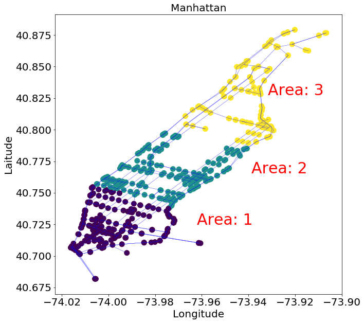
Manhattan Mobility Model maps are generated from the real road data of Manhattan from INRIX111© 2024 INRIX, Inc.,”INRIX documentation,” INRIX documentation https://docs.inrix.com/., which is shown in Fig.1. We follow the setting of Manhattan Mobility Model from bai2003important: a vehicle is allowed to move along the grid of horizontal and vertical streets on the map. At an intersection, the vehicle can turn left, right or go straight. This choice is probabilistic: the probability of moving on the same street is 0.5, and the probabilities of turn into one of the rest roads are equal. For example, at an intersection with 3 more roads to turn into, then the probability to turn into each road is 0.1667. Follow the setting from su2022boost: each vehicle is equipped with DSRC and mmWave communication components, can communicate to other vehicles within the communication range of 100 meters, while the default velocity of each vehicle is 13.89 m/s. In our experiment, we set up the number of local updates , and the interval between each epoch is seconds. Within each global epoch, vehicles train their models on local datasets while moving on the road and updating their cache by uploading and downloading models with other encountered vehicles.
4.5 LRU Cache Update
Algorithm 2, which we name as LRU method for convenience, is the basic cache update method we proposed. Basically, the LRU updating rule aims to fetch the most-up-to-date models and keep as many of them in the cache as possible. At line 13, 18, the metric for making choice among models is the timestamp of models, which is defined as the epoch time when the model was received from the original vehicle, rather than received from the cache. What’s more, to fully utilize the caching mechanism, a vehicle not only fetches other vehicles’ own trained models, but also models in their caches. For instance, at epoch , vehicle can directly fetch model from vehicle , at line 7, and also fetch models from the cache of vehicle , at line 8. This way, each vehicle can not only fetch the models directly from its neighbours, but also indirectly from its neighbours’ neighbours, thus boosting the spreading of the underlying data information from different vehicles, and improving the DFL convergence speed, especially with heterogeneous data distribution. Additionally, at line 2, before updating cache, models with staleness will be removed from each vehicle’s cache.

5 Numerical Results
5.1 Caching vs. Non-caching
To evaluate the performance of DFedCache, we compare the DFL with LRU Cache, Centralized FL (CFL) and DFL on MNSIT, FashionMNIST, CIFAR-10 with three distributions: non-i.i.d, i.i.d, Dirichlet with . For LRU update, we take the cache size as 10 for MNIST and FashionMNIST, and 3 for CIFAR-10 and based on practical considerations. Given a speed of and and a communication distance of , the communication window of two agents driving in opposite directions could be limited. Additionally, considering the size of chosen models and communication overhead, the above cache sizes were chosen. From the results in Fig. 2, we can see that DFedCache boosts the convergence and outperforms non-caching method (DFL) and gains performance much closer to CFL in all the cases, especially in non-i.i.d. scenarios.
5.2 Impact of Cache Size
Then we evaluate the performance gains with different cache sizes from 1 to 30 and , on MNIST and FashionMNIST in Fig. 3. LRU can benefit more from larger cache sizes, especially in non-i.i.d scenarios, as aggregation with more cached models gets closer to CFL and training with global data distribution.

5.3 Impact of Model Staleness
As mentioned in the previous sections, one drawback of model caching is introducing stale models into aggregation, so it is very important to choose a proper staleness tolerance . First, we statistically calculate the relation between the average number and the average age of cached models at different from 1 to 20, when epoch time is 30s, 60s, 120s, with unlimited cache size, in Table 2. We can see that, with the fixed epoch time, as the increases, the average number and average age of cached models increase, approximately linearly. It’s not hard to understand, as every epoch each agent can fetch a limited number of models directly from other agents. Increasing the staleness tolerance will increase the number of cached models, as well as the age of cached models. What’s more, we can see that the communication frequency or the moving speed of agents will also impact the average age of cached models, as the faster an agent moves, the more models it can fetch within each epoch, which we will further discuss later.
| 1 | 2 | 3 | 4 | 5 | 10 | 20 | ||
|---|---|---|---|---|---|---|---|---|
| 30s | num | 0.8549 | 1.6841 | 2.6805 | 3.8584 | 5.2054 | 14.8520 | 44.8272 |
| age | 0.0000 | 0.4904 | 1.0489 | 1.6385 | 2.2461 | 5.4381 | 11.5735 | |
| 60s | num | 1.6562 | 3.8227 | 6.4792 | 10.3889 | 14.0749 | 43.0518 | 90.2576 |
| age | 0.000 | 0.5593 | 1.1604 | 1.8075 | 2.4396 | 5.5832 | 9.7954 | |
| 120s | num | 3.6936 | 9.9149 | 18.5016 | 31.3576 | 35.1958 | 90.2469 | 98.5412 |
| age | 0.0000 | 0.6189 | 1.2715 | 1.9194 | 1.5081 | 4.7131 | 5.2357 |
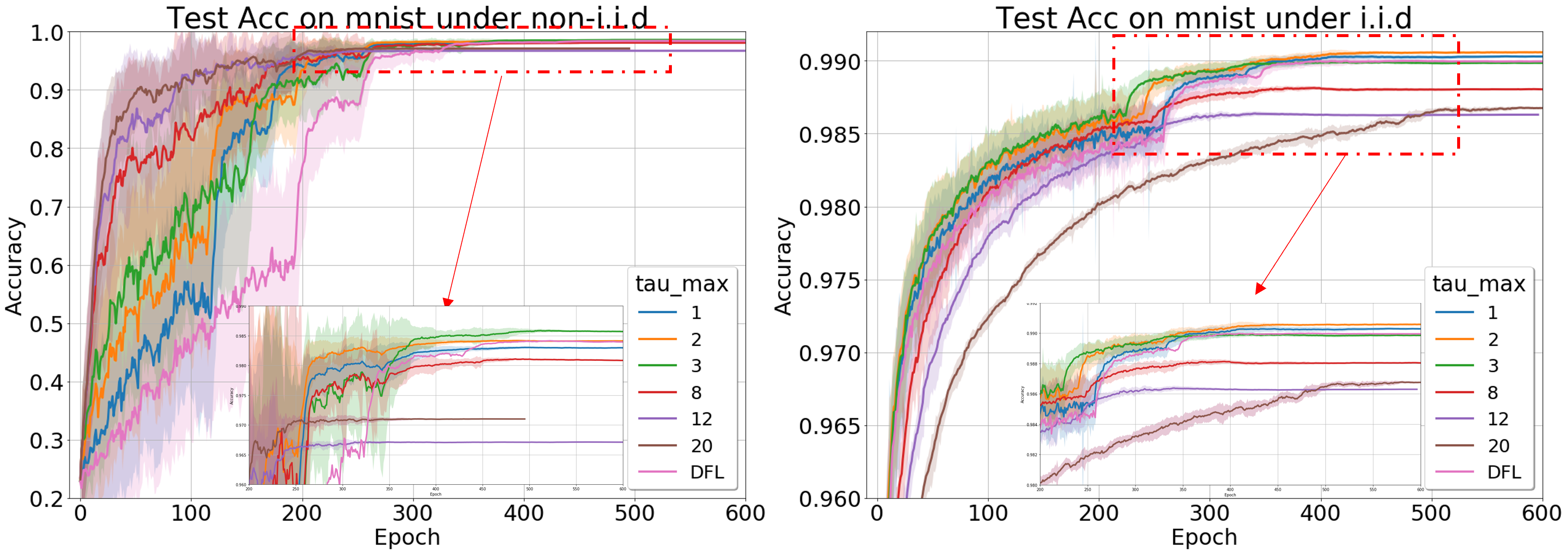
And we also compare the performance of DFL with LRU at different on MNIST under non-i.i.d and i.i.d in Fig.4. Here we pick the epoch time 30s for a clear view. First, for non-i.i.d, the larger brings faster convergence at the beginning, which is consistent with our previous conclusion, as it allows more cached models which bring more benefits than harm to the training with non-i.i.d. However, for i.i.d scenario, larger stops improving the performance of models, as introducing more cached models hardly benefits training in i.i.d, and the model staleness will prevent the convergence. What’s more, if we zoom in the final converging phase, which is amplified in the bottom of each figure, we observe that larger will reduce the final converged accuracy in both non-i.i.d and i.i.d scenarios, as it introduces more staleness. Even with large and large staleness, LRU method still achieves similar or even better performance than DFL in non-i.i.d. scenarios.

5.4 Mobility’s Impact on Convergence
Vehicle mobility directly determines the frequency and efficiency of cache-based model spreading and aggregation. So we evaluate the performance of cached DFL at different vehicle speeds. We fix cache size at 10, with non-i.i.d. data distribution. We take the our previous speed and local updates as the base, named as speedup x1. To speedup, increases while reduces to keep the fair comparison under the same wall clock. For instance, for speedup x3, and . Results in Fig. 5 shows that when the mobility speed increases, although the number of local updates decreases, the spread of all models in the whole vehicle network is boosted, thus disseminating local models more quickly among all vehicles, leading to faster model convergence.

5.5 Experiments with Grouped Mobility Patterns and Data Distributions
In practice, vehicle mobility patterns and local data distributions may naturally form groups. For example, a vehicle may mostly move within its home area, and collect data specific to that area. Vehicles within the same area meet with each others frequently, but have very similar data distributions. A fresh model of a vehicle in the same area is not as valuable as a slightly older model of a vehicle from another area. So model caching should not just consider model freshness, but should also take into account the coverage of group-based data distributions. For those scenarios, we develop a Group-based (GB) caching algorithm as Algorithm 3. More specifically, knowing that there are distribution groups, one should maintain balanced presences of models from different groups. One straightforward extension of the LRU caching algorithm is to partition the cache into sub-caches, one for each group. Each sub-cache is updated by local models from its associated group, using the LRU policy.
Input: Current cache , Cache of device : , Model from device , Current time , Cache size , Tolerance of staleness , Device group mapping list , here . Group cache size list , here is number of cache slots reserved for models from devices belong to group .
Here the model is local updated at time , based on car ’s dataset.
Output:
We now conduct a case study for group-based cache update. As shown in Fig 1, the whole Manhattan road network is divided into 3 areas, downtown, mid-town and uptown. Each area has 30 area-restricted vehicles that randomly moves within that area, and 3 or 4 free vehicles that can move into any area. We set 4 different area-related data distributions: Non-overlap, 1-overlap, 2-overlap, 3-overlap. -overlap means the number of shared labels between areas is . We use the same non-i.i.d shards method in the previous section to allocate data points to the vehicles in the same area. On each vehicle, we evenly divide the cache for the three areas. We evaluate our proposed GB cache method on FashionMNIST. As shown in Fig. 6, while vanilla LRU converges faster at the very beginning, it cannot outperform DFL at last. However, the GB update method can solve the problem of LRU update and outperform DFL under different overlap settings.

5.6 Discussions
In general, the convergence rate of DFedCache outperforms non-caching method (DFL), especially for non-i.i.d. distributions. Larger cache size and smaller make DFedCache closer to the performance of CFL. Empirically, there is a trade-off between the age and number of cached models, it is critical to choose a proper to control the staleness. What’s more, the choice of should take into account the diversity data distributions on agents. In general, with non-i.i.d data distributions, the benefits of increasing the number of cached models can outweigh the damages caused by model staleness; while when data distributions are close to i.i.d, it is better to use a small number of fresh models than a large number of stale models. Similarly conclusions can also be drawn from the results of area-restricted vehicles. What’s more, in a system of moving agents, the mobility will also have big impact on the training, usually higher speed and communication frequency improve the model convergence and accuracy.
6 Related Work
Decentralized FL (DFL) has been increasingly applied in vehicular networks, leveraging existing frameworks like vehicle-to-vehicle (V2V) communication [yuan2024decentralized]. V2V FL facilitates knowledge sharing among vehicles and has been explored in various studies [samarakoon2019distributed, pokhrel2020decentralized, yu2020proactive, chen2021bdfl, barbieri2022decentralized, su2022boost]. samarakoon2019distributed studied optimized joint power and resource allocation for ultra-reliable low-latency communication (URLLC) using FL.
su2022boost introduced DFL with Diversified Data Sources to address data diversity issues in DFL, improving model accuracy and convergence speed in vehicular networks. None of the previous studies explored model caching on vehicles. Convergence of asynchronous federated optimization was studied in DBLP:journals/corr/abs-1903-03934. Their analysis focused on pairwise model aggregation between an agent and the parameter server, does not cover decentralized model aggregation with stale cached models in our proposed framework.
7 Conclusion & Future Work
In this paper, we developed a novel decentralized federated learning framework that leverages on model caching on mobile agents for fast and even model spreading. We theoretically analyzed the convergence of DFL with cached models. Through extensive case studies in a vehicle network, we demonstrated that our algorithm significantly outperforms DFL without model caching, especially for agents with non-i.i.d data distributions. We employed only simple model caching and aggregation algorithms in the current study. We will investigate more refined model caching and aggregation algorithms customized for different agent mobility patterns and non-i.i.d. data distributions.
References
- Bai et al. [2003] Fan Bai, Narayanan Sadagopan, and Ahmed Helmy. Important: A framework to systematically analyze the impact of mobility on performance of routing protocols for adhoc networks. In IEEE INFOCOM 2003. Twenty-second Annual Joint Conference of the IEEE Computer and Communications Societies (IEEE Cat. No. 03CH37428), volume 2, pages 825–835. IEEE, 2003.
- Barbieri et al. [2022] Luca Barbieri, Stefano Savazzi, Mattia Brambilla, and Monica Nicoli. Decentralized federated learning for extended sensing in 6g connected vehicles. Vehicular Communications, 33:100396, 2022.
- Burleigh et al. [2003] Scott Burleigh, Adrian Hooke, Leigh Torgerson, Kevin Fall, Vint Cerf, Bob Durst, Keith Scott, and Howard Weiss. Delay-tolerant networking: an approach to interplanetary internet. IEEE Communications Magazine, 41(6):128–136, 2003.
- Chen et al. [2021] Jin-Hua Chen, Min-Rong Chen, Guo-Qiang Zeng, and Jia-Si Weng. Bdfl: A byzantine-fault-tolerance decentralized federated learning method for autonomous vehicle. IEEE Transactions on Vehicular Technology, 70(9):8639–8652, 2021.
- Deng [2012] Li Deng. The mnist database of handwritten digit images for machine learning research [best of the web]. IEEE signal processing magazine, 29(6):141–142, 2012.
- He et al. [2016] Kaiming He, Xiangyu Zhang, Shaoqing Ren, and Jian Sun. Deep residual learning for image recognition. In Proceedings of the IEEE conference on computer vision and pattern recognition, pages 770–778, 2016.
- Krizhevsky [2009] A Krizhevsky. Learning multiple layers of features from tiny images. Master’s thesis, University of Tront, 2009.
- Liu et al. [2022] Ji Liu, Jizhou Huang, Yang Zhou, Xuhong Li, Shilei Ji, Haoyi Xiong, and Dejing Dou. From distributed machine learning to federated learning: A survey. Knowledge and Information Systems, 64(4):885–917, 2022.
- Martínez Beltrán et al. [2023] Enrique Tomás Martínez Beltrán, Mario Quiles Pérez, Pedro Miguel Sánchez Sánchez, Sergio López Bernal, Gérôme Bovet, Manuel Gil Pérez, Gregorio Martínez Pérez, and Alberto Huertas Celdrán. Decentralized federated learning: Fundamentals, state of the art, frameworks, trends, and challenges. IEEE Communications Surveys & Tutorials, 25(4):2983–3013, 2023. doi: 10.1109/COMST.2023.3315746.
- McMahan et al. [2017] Brendan McMahan, Eider Moore, Daniel Ramage, Seth Hampson, and Blaise Aguera y Arcas. Communication-efficient learning of deep networks from decentralized data. In Artificial intelligence and statistics, pages 1273–1282. PMLR, 2017.
- Niknam et al. [2020] Solmaz Niknam, Harpreet S Dhillon, and Jeffrey H Reed. Federated learning for wireless communications: Motivation, opportunities, and challenges. IEEE Communications Magazine, 58(6):46–51, 2020.
- Paszke et al. [2017] Adam Paszke, Sam Gross, Soumith Chintala, Gregory Chanan, Edward Yang, Zachary DeVito, Zeming Lin, Alban Desmaison, Luca Antiga, and Adam Lerer. Automatic differentiation in pytorch. 2017.
- Pokhrel and Choi [2020] Shiva Raj Pokhrel and Jinho Choi. A decentralized federated learning approach for connected autonomous vehicles. In 2020 IEEE Wireless Communications and Networking Conference Workshops (WCNCW), pages 1–6. IEEE, 2020.
- Robbins and Monro [1951] Herbert Robbins and Sutton Monro. A stochastic approximation method. The annals of mathematical statistics, pages 400–407, 1951.
- Samarakoon et al. [2019] Sumudu Samarakoon, Mehdi Bennis, Walid Saad, and Mérouane Debbah. Distributed federated learning for ultra-reliable low-latency vehicular communications. IEEE Transactions on Communications, 68(2):1146–1159, 2019.
- Shokri and Shmatikov [2015] Reza Shokri and Vitaly Shmatikov. Privacy-preserving deep learning. In Proceedings of the 22nd ACM SIGSAC conference on computer and communications security, pages 1310–1321, 2015.
- Su et al. [2022] Dongyuan Su, Yipeng Zhou, and Laizhong Cui. Boost decentralized federated learning in vehicular networks by diversifying data sources. In 2022 IEEE 30th International Conference on Network Protocols (ICNP), pages 1–11. IEEE, 2022.
- Sun et al. [2022] Tao Sun, Dongsheng Li, and Bao Wang. Decentralized federated averaging. IEEE Transactions on Pattern Analysis and Machine Intelligence, 2022.
- Xiao et al. [2017] Han Xiao, Kashif Rasul, and Roland Vollgraf. Fashion-mnist: a novel image dataset for benchmarking machine learning algorithms, 2017. URL https://arxiv.org/abs/1708.07747.
- Xie et al. [2019] Cong Xie, Sanmi Koyejo, and Indranil Gupta. Asynchronous federated optimization. CoRR, abs/1903.03934, 2019. URL http://arxiv.org/abs/1903.03934.
- Xiong et al. [2024] Guojun Xiong, Gang Yan, Shiqiang Wang, and Jian Li. Deprl: Achieving linear convergence speedup in personalized decentralized learning with shared representations. In Proceedings of the AAAI Conference on Artificial Intelligence, volume 38, pages 16103–16111, 2024.
- Yang et al. [2021] Haibo Yang, Minghong Fang, and Jia Liu. Achieving linear speedup with partial worker participation in non-iid federated learning. Proceedings of ICLR, 2021.
- Yu et al. [2020] Zhengxin Yu, Jia Hu, Geyong Min, Han Xu, and Jed Mills. Proactive content caching for internet-of-vehicles based on peer-to-peer federated learning. In 2020 IEEE 26th International Conference on Parallel and Distributed Systems (ICPADS), pages 601–608. IEEE, 2020.
- Yuan et al. [2024] Liangqi Yuan, Ziran Wang, Lichao Sun, S Yu Philip, and Christopher G Brinton. Decentralized federated learning: A survey and perspective. IEEE Internet of Things Journal, 2024.
- Zhang et al. [2019] Michael Zhang, James Lucas, Jimmy Ba, and Geoffrey E Hinton. Lookahead optimizer: k steps forward, 1 step back. Advances in neural information processing systems, 32, 2019.
Appendix A Convergence Analysis
We now theoretically investigate the impact of caching, especially the staleness of cached models, on DFL model convergence. We introduce some definitions and assumptions.
Definition 4 (Smoothness).
A differentiable function is -smooth if for , where .
Definition 5 (Bounded Variance).
There exists a constant such that the global variability of the local gradient of the loss function is bounded .
Definition 6 (L-Lipschitz Continuous Gradient).
There exists a constant , such that
Theorem 5.
Assume that is -smooth and convex, and each agent executes local updates before meeting and exchanging models, after that, then does model aggregation. We also assume bounded staleness , as the kick-out threshold. Furthermore, we assume, , and , and satisfies L-Lipschitz Continuous Gradient. For any small constant , if we take , and satisfying , after global epochs, Algorithm 1 converges to a critical point:
A.1 Proof
Similar to Theorem 1 in [DBLP:journals/corr/abs-1903-03934], we can get the boundary before and after times local updates on -th device, :
| (5) |
For any epoch , we find the index of the agent whose model is the “worst", i.e., , then we can get,
| (6) |
here .
We can easy know, for given , we have , then,
| (7) |
Here , so we rearrange the equation above, we can get:
| (8) |
We define the “worst" model on all agents over the time period of as
Then we can get,
| (9) |
Here, , so we have,
| (10) |
Then,
| (11) |
By taking use of the property of L-Lipschitz Continuous Gradient, we can get,
| (12) |
Then, we can get, , , then
| (13) |
So we have,
| (14) |
We assume the ratio of gradient expectation on the global distribution to gradient expectation on local data distribution of any device is bounded, i.e.,
| (15) |
So we get,
| (16) |
Inequality (A.1) becomes:
| (17) |
By rearranging the terms, we have,
| (18) |
We iteratively construct a time sequence in the backward fashion so that
From the equation above, we can also get the inequality about ,
| (19) |
Applying inequality (A.1) at all time instances , after T global epochs, we have,
| (20) |
With the results in (A.1) and by leveraging Theorem 1 in yang2021achieving, Algorithm 1 converges to a critical point after global epochs.
Appendix B Experimental details
B.1 Data distribution in Group-based LRU Cache Experiment
B.1.1 -overlap
For MNIST, FashionMNIST with 10 classes labels, we allocate labels into 3 groups as:
Non-overlap:
Area 1: (0,1,2,3), Area 2: (4,5,6), Area 3: (7,8,9)
1-overlap:
Area 1: (9,0,1,2,3), Area 2: (3,4,5,6), Area 3: (6,7,8,9)
2-overlap:
Area 1: (8,9,0,1,2,3), Area 2: (2,3,4,5,6), Area 3: (5,6,7,8,9)
3-overlap:
Area 1: (7,8,9,0,1,2,3), Area 2: (1,2,3,4,5,6), Area 3: (4,5,6,7,8,9)
B.2 Computing infrastructure
For MNIST and FashionMNIST experiments, we use 10 computing nodes, each with 10 CPUs, model: Lenovo SR670, to simulate DFL on 100 vehicles. CIFAR-10 results are obtained from 1 compute node with 5 CPUs and 1 A100 NVIDIA GPU, model: SD650-N V2. They are all using Ubuntu-20.04.1 system with pre-installed openmpi/intel/4.0.5 module, and 100 Gb/s network speed.
B.3 Results with variation
As our metric is the average test accuracy over 100 devices, we also provide the variation of the average test accuracy in our experimental results as following,


| 1 | 2 | 3 | 4 | 5 | 10 | 20 | ||
|---|---|---|---|---|---|---|---|---|
| 30s | num | 0.8549 | 1.6841 | 2.6805 | 3.8584 | 5.2054 | 14.8520 | 44.8272 |
| 0.0321 | 0.0903 | 0.1941 | 0.3902 | 0.6986 | 6.2270 | 42.8144 | ||
| age | 0.0000 | 0.4904 | 1.0489 | 1.6385 | 2.2461 | 5.4381 | 11.5735 | |
| 0.0000 | 0.0052 | 0.0116 | 0.0203 | 0.0320 | 0.1577 | 1.0520 | ||
| 60s | num | 1.6562 | 3.8227 | 6.4792 | 10.3889 | 14.0749 | 43.0518 | 90.2576 |
| 0.0865 | 0.3594 | 0.9925 | 2.824 | 5.1801 | 32.8912 | 55.5829 | ||
| age | 0.000 | 0.5593 | 1.1604 | 1.8075 | 2.4396 | 5.5832 | 9.7954 | |
| 0.0000 | 0.0035 | 0.0089 | 0.0188 | 0.0251 | 0.1448 | 0.8375 | ||
| 120s | num | 3.6936 | 9.9149 | 18.5016 | 31.3576 | 35.1958 | 90.2469 | 98.5412 |
| 0.3166 | 2.3825 | 5.9696 | 21.7408 | 56.8980 | 28.8958 | 29.9676 | ||
| age | 0.0000 | 0.6189 | 1.2715 | 1.9194 | 1.5081 | 4.7131 | 5.2357 | |
| 0.0000 | 0.0028 | 0.0058 | 0.0212 | 0.9742 | 0.1249 | 0.1808 |


B.4 Final (hyper-)parameters in experiments
learning rate , batch size = 64. For all the experiments, we train for 1,000 global epochs, and implement early stop when the average test accuracy stops increasing for at least 20 epochs. Without specific explanation, we take the following parameters as the final default parameters in our experiments. Local epoch , vehicle speed , communication distance , communication interval between each epoch , , number of devices , cache size .
B.5 NN models
We choose the models from the classical repository 222 Federated-Learning-PyTorch , Implementation of Communication-Efficient Learning of Deep Networks from Decentralized Data © 2024 GitHub, Inc.https://github.com/AshwinRJ/Federated-Learning-PyTorch.: we run convolutional neural network (CNN) as shown in Table 4, for MNIST, convolutional neural network (CNN) as shown in Table 5, for FashionMNIST. Inspired by [zhang2019lookahead], we choose ResNet-18 for Cifar-10, as shown in Table 6.
| Layer Type | Size |
|---|---|
| Convolution + ReLU | |
| Max Pooling | |
| Convolution + ReLU + Dropout | |
| Dropout(2D) | |
| Max Pooling | |
| Fully Connected + ReLU | |
| Dropout | |
| Fully Connected |
| Layer Type | Size |
|---|---|
| Convolution + BatchNorm + ReLU | |
| Max Pooling | |
| Convolution + BatchNorm + ReLU | |
| Max Pooling | |
| Fully Connected |
| Layer Type | Output Size |
|---|---|
| Convolution + BatchNorm + ReLU | |
| Residual Block 1 (2x BasicBlock) | |
| Residual Block 2 (2x BasicBlock) | |
| Residual Block 3 (2x BasicBlock) | |
| Residual Block 4 (2x BasicBlock) | |
| Average Pooling | |
| Fully Connected |