This paper was converted on www.awesomepapers.org from LaTeX by an anonymous user.
Want to know more? Visit the Converter page.

Decentralized Concurrent Learning with Coordinated Momentum and Restart

Daniel E. Ochoa Muhammad U. Javed Xudong Chen Jorge I. Poveda Department of Electrical and Computer Engineering, University of California, San Diego, La Jolla, CA 92093 Department of Electrical, Computer and Energy Engineering, University of Colorado, Boulder, CO 80309 Department of Electrical and Systems Engineering, Washington University in St. Louis, MO 63112
Abstract

This paper studies the stability and convergence properties of a class of multi-agent concurrent learning (CL) algorithms with momentum and restart. Such algorithms can be integrated as part of the estimation pipelines of data-enabled multi-agent control systems to enhance transient performance while maintaining stability guarantees. However, characterizing restarting policies that yield stable behaviors in decentralized CL systems, especially when the network topology of the communication graph is directed, has remained an open problem. In this paper, we provide an answer to this problem by synergistically leveraging tools from graph theory and hybrid dynamical systems theory. Specifically, we show that under a cooperative richness condition on the overall multi-agent system’s data, and by employing coordinated periodic restart with a frequency that is tempered by the level of asymmetry of the communication graph, the resulting decentralized dynamics exhibit robust asymptotic stability properties, characterized in terms of input-to-state stability bounds, and also achieve a desirable transient performance. To demonstrate the practical implications of the theoretical findings, three applications are also presented: cooperative parameter estimation over networks with private data sets, cooperative model-reference adaptive control, and cooperative data-enabled feedback optimization of nonlinear plants.

keywords:
Concurrent Learning, Data-driven Optimization, Multi-Agent Systems, Hybrid Dynamical Systems
journal: arXiv

1 INTRODUCTION

Concurrent Learning (CL) techniques have emerged as powerful data-driven tools for designing estimation and learning dynamics in a wide range of applications where persistence of excitation (PE) conditions are either impractical or infeasible [1, 2]. These techniques have demonstrated their utility in diverse fields, including parameter estimation in batteries [3], exoskeleton robotic systems [4, 5], mobile robots and aerial vehicles [6], extremum seeking algorithms [7], and reinforcement learning controllers [8, 9]. In these applications, extensive datasets containing historical recorded measurements of the relevant system signals are often available and can be leveraged for estimation purposes. When these datasets are “sufficiently rich”, they can be seamlessly integrated into dynamic estimation algorithms, enabling (uniform) exponential convergence to the unknown parameters even in the absence of PE conditions.

However, relaxations of PE conditions can lead to suboptimal transient performance, particularly in terms of slow convergence rates that depend on the “level of richness” of the dataset used by the algorithm. Since datasets readily available in applications may exhibit prohibitively small levels of richness, there is a growing need for the development of enhanced CL techniques that can accelerate the convergence rate of the estimation dynamics while maintaining the desirable stability and robustness properties.

1.1 Literature Review

One promising direction to alleviate the slow convergence issue in decision-making algorithms is the incorporation of momentum with dynamic damping, see [3, 10, 11]. For single-agent gradient-based dynamics with momentum, the use of decreasing damping has been shown to play a crucial role in inducing favorable acceleration properties [12, 13, 14, 15]. However, it has also been shown that stability bounds in terms of 𝒦\mathcal{KL} functions may not exist for such systems unless the damping coefficients are persistently exciting [16], a condition that precludes vanishing coefficients. Furthermore, it is well-known that, without proper tuning, the use of momentum can lead to undesirable oscillations [17]. To address potential instability issues and to eliminate oscillatory behaviors, restart mechanisms that reset the momentum have been developed for single-agent systems using adaptive [17, 18] and periodic policies (usually called “scheduled”) with carefully selected frequencies [13, 19, 20, 17]. Recent works have also investigated the development of similar momentum-based algorithms in multi-agent systems, including distributed continuous-time heavy-ball dynamics with constant damping [21], limiting equations of stochastic recursive algorithms as multi-agent flows with momentum [22], and decision-making algorithms with momentum for high-order multi-agent systems [23, 24, 25]. However, existing approaches have primarily focused on undirected network topologies. Additionally, the incorporation of momentum and restarting mechanisms in decentralized concurrent learning algorithms has remained unexplored. Such algorithms are essential when a network of agents seeks to collaboratively and efficiently learn a common model by sharing local estimates with neighboring agents, without revealing their private data. Applications of these algorithms span various domains, including source seeking in autonomous mobile robots [26], adaptive formation control of robotic teams [27], and cooperative adaptive control [28].

1.2 Contributions

Motivated by the previous background, in this paper we study the synthesis and analysis of decentralized concurrent learning dynamics with momentum and restart for general directed graphs. In particular, we consider a model that extends the centralized dynamics studied in [13, 14], and [19] to cases where each agent implements its own restart policy and shares information only with neighbors characterized by the topology of the communication graph. To assess the impact of the topology of graph on the stability properties of the dynamics, we exploit analytical tools from graph theory and hybrid dynamical system’s theory [29]. Using these tools, this paper makes the following primary contributions:

(1) We first introduce a class of multi-agent concurrent learning (CL) algorithms that incorporate momentum and a centralized restarting mechanism. We demonstrate that if: (a) the graph is strongly connected, (b) the overall data collected by the agents satisfies a “cooperative richness condition,” and (c) the restarting frequency exceeds a certain threshold that encodes the “asymmetry” of the communication graph, then the resulting error estimation dynamics are input-to-state stable [30] with respect to measurement noise and model error approximations. Furthermore, the convergence is exponential with rates assignable via the restarting period. These results are presented in Theorem 1.

(2) Next, by leveraging the robustness properties of the dynamics, we interconnect the momentum-based concurrent learning algorithms with a decentralized coordinated restarting mechanism, enabling a fully decentralized implementation. The resulting dynamical systems are also globally stable and exhibit convergence rates consistent with Theorem 1 following an initial synchronization phase of the restarting times. These results are presented in Theorem 2.

(3) Finally, we present three applications of the proposed momentum-based CL algorithms with restart within the context of data-enabled control: (a) cooperative parameter estimation without persistently exciting regressors in networks where nodes have private data with heterogeneous informativity properties; (b) data-enabled cooperative model-reference adaptive control; (c) data-enabled cooperative feedback-optimization. By employing (hybrid) Lyapunov-based techniques, we show that the resulting closed-loop systems exhibit favorable stability and convergence properties, which are also illustrated via numerical examples.

The rest of this paper is organized as follows: Section 2 presents the preliminaries. Section 3 presents the problem formulation. Section 4 presents the main results. Section 5 presents applications, Section 6 includes the proofs, and Section 7 concludes the paper.

2 Preliminaries

Notation: We use r𝔹r\mathbb{B} to denote a closed ball of appropriate dimension in the Euclidean space, of radius r>0r>0, and centered at the origin. Let EijE_{ij} be the matrix with all entries equal to zero except the ijthij^{\text{th}} entry, which is equal to one. Let 𝟏nn\mathbf{1}_{n}\in\mathbb{R}^{n} be the vector of all ones, and Inn×nI_{n}\in\mathbb{R}^{n\times n} be the identity matrix. Given x,ynx,y\in\mathbb{R}^{n}, we let (x,y)[x,y](x,y)\coloneqq[x^{\top},y^{\top}]^{\top} denote their concatenation. We use {e1,e2,,en}\{e_{1},e_{2},\ldots,e_{n}\} to denote the standard basis of n\mathbb{R}^{n}. A matrix MN×NM\in\mathbb{R}^{N\times N} is represented in terms of its entries as M=[mij]M=[m_{ij}], with mijm_{ij}\in\mathbb{R} being its ijthij^{\text{th}} entry. Similarly, we use 𝐌=[𝐌ij]\mathbf{M}=[\mathbf{M}_{ij}] to represent a block matrix 𝐌\mathbf{M} in terms of its blocks, and use diag({M1,,MJ})\text{diag}\left(\{M_{1},\ldots,M_{J}\}\right) to build a block diagonal matrix from the set of matrices {Mj}j=1J\{M_{j}\}_{j=1}^{J}. Given a vector xnx\in\mathbb{R}^{n} we let diag(x)\text{diag}(x) represent a diagonal matrix with diagonal entries (i,i)(i,i) given by the ithi^{th} entry of xx. A matrix B=[bij]N×N,B=[b_{ij}]\in\mathbb{R}^{N\times N}, is said to be nonnegative (B0B\geq 0) if bij0b_{ij}\geq 0 for all i,ji,j. The spectral radius of a matrix BB is denoted by ρ(B)\rho(B). We use |||\cdot| for the vector 2-norm, \|\cdot\| for the matrix norm induced by |||\cdot|, and |z|𝒜infs𝒜|zs||z|_{\mathcal{A}}\coloneqq\inf_{s\in\mathcal{A}}|z-s| to denote the distance of a vector znz\in\mathbb{R}^{n} to a closed set 𝒜n\mathcal{A}\subset\mathbb{R}^{n}. With a slight abuse of notation, given a matrix 𝐏0\mathbf{P}\succeq 0 we define the semi-norm |x|𝐏(x𝐏x)1/2|x|_{\mathbf{P}}\coloneqq(x^{\top}\mathbf{P}x)^{1/2}. Given a set-valued mapping M:mnM:\mathbb{R}^{m}\rightrightarrows\mathbb{R}^{n}, the domain of MM is the set dom(M)={xm:M(x)}\text{dom}(M)=\{x\in\mathbb{R}^{m}~{}:~{}M(x)\neq\emptyset\}. A function γ:00\gamma:\mathbb{R}_{\geq 0}\to\mathbb{R}_{\geq 0} is of class 𝒦\mathcal{K} (γ𝒦\gamma\in\mathcal{K}) if it is continuous, strictly increasing, and satisfies γ(0)=0\gamma(0)=0. It is said to be of class 𝒦\mathcal{K}_{\infty} (γ𝒦\gamma\in\mathcal{K}_{\infty}), if additionally γ(r)\gamma(r)\to\infty as rr\to\infty. A function β:0×00\beta:\mathbb{R}_{\geq 0}\times\mathbb{R}_{\geq 0}\to\mathbb{R}_{\geq 0} is of class 𝒦\mathcal{K}\mathcal{L} (β𝒦\beta\in\mathcal{KL}) if it is nondecreasing in its first argument, nonincreasing in its second argument, limr0+β(r,s)=0\lim_{r\to 0^{+}}\beta(r,s)=0 for each s0s\in\mathbb{R}_{\geq 0}, and limsβ(r,s)=0\lim_{s\to\infty}\beta(r,s)=0 for each r0r\in\mathbb{R}_{\geq 0}.

Graph Theory: For a directed graph (digraph) 𝒢=(𝒱,)\mathcal{G}=(\mathcal{V},\mathcal{E}), we denote by (i,j)(i,j)\in\mathcal{E} a directed edge from node ii to node jj, we call node ii an in-neighbor of node jj, and we call node jj an out-neighbor of node ii. We consider digraphs that do not have self-arcs. A weighted Laplacian matrix =[lij]N×N\mathcal{L}=[l_{ij}]\in\mathbb{R}^{N\times N} associated with 𝒢\mathcal{G} satisfies the following: the off-diagonal entries are such that lij<0l_{ij}<0 if (i,j)(i,j) is an edge, and lij=0l_{ij}=0 otherwise; the diagonal entries liil_{ii} are determined such that every row of \mathcal{L} sums to zero, and all its nonzero eigenvalues have positive real part [31, Lemma 6.5]. A digraph is strongly connected if for any two distinct nodes ii and jj, there is a path from ii to jj. The Laplacian matrix of a strongly connected digraph satisfies rank()=N1\text{rank}(\mathcal{L})=N-1 [31, Ch. 6].

Hybrid Dynamical Systems: In this paper, we work with dynamical systems that combine continuous-time and discrete-time dynamics. Such systems are called hybrid dynamical systems (HDS) [29]. The dynamics of a HDS with state xnx\in\mathbb{R}^{n} are represented as:

(x,u)CCx×m,x˙F(x,u),\displaystyle(x,u)\in C\coloneqq C_{x}\times\mathbb{R}^{m},~{}~{}~{}~{}~{}\dot{x}\in F(x,u), (1a)
(x,u)DDx×m,x+G(x),\displaystyle(x,u)\in D\coloneqq D_{x}\times\mathbb{R}^{m},~{}~{}~{}~{}x^{+}\in G(x), (1b)

where umu\in\mathbb{R}^{m} is an exogenous input, F:n×mnF:\mathbb{R}^{n}\times\mathbb{R}^{m}\rightrightarrows\mathbb{R}^{n} is called the flow map, G:nnG:\mathbb{R}^{n}\rightrightarrows\mathbb{R}^{n} is called the jump map, Cn×mC\subset\mathbb{R}^{n}\times\mathbb{R}^{m} is called the flow set, and Dn×mD\subset\mathbb{R}^{n}\times\mathbb{R}^{m} is called the jump set. We use =(C,F,D,G,u)\mathcal{H}=(C,F,D,G,u) to denote the data of the HDS \mathcal{H}. These systems generalize purely continuous-time systems (D~=\tilde{D}=\emptyset) and purely discrete-time systems (C~=\tilde{C}=\emptyset). Time-varying systems can also be represented as (1) by using an auxiliary state ss\in\mathbb{R} with dynamics s˙>0\dot{s}>0 and s+=ss^{+}=s. Solutions to system (1) are parameterized by a continuous-time index t0t\in\mathbb{R}_{\geq 0}, which increases continuously during flows, and a discrete-time index j0j\in\mathbb{Z}_{\geq 0}, which increases by one during jumps. Therefore, solutions to (1) are defined on hybrid time domains (HTDs). Solutions to (1) are required to satisfy dom(x)=dom(u)\text{dom}(x)=\text{dom}(u), with u(,j)u(\cdot,j) being locally essentially bounded and Lebesgue measurable for each jj. To establish this correspondence, a hybrid input uu in (1) is obtained from a suitable continuous-time input uu by using (with some abuse of notation) u(t,j)=u(t)u(t,j)=u(t) during the flows (1a) for each fixed jj, and by keeping uu constant during the jumps (1b). For a precise definition of hybrid time domains and solutions to HDS of the form (1), we refer the reader to [32]. To simplify notation, in this paper we use |u|(t,j)=esssup(0,0)(t~,j~)(t,j)|u(t~,j~)||u|_{(t,j)}=\operatorname*{ess\,sup}_{\begin{subarray}{c}(0,0)\preceq(\tilde{t},\tilde{j})\preceq(t,j)\end{subarray}}\left|u(\tilde{t},\tilde{j})\right|, and we let |u|limt+j|u|(t,j)|u|_{\infty}\coloneqq\lim_{t+j\to\infty}|u|_{(t,j)}. The stability properties of HDS will be studied using the following notion.

Definition 1

Given a closed set 𝒜CxDx\mathcal{A}\subset C_{x}\cup D_{x}, a HDS \mathcal{H} of other form (1) is said to be input-to-state stable (ISS) with respect to ||𝒜|\cdot|_{\mathcal{A}} if there exist β𝒦\beta\in\mathcal{KL} and γ𝒦\gamma\in\mathcal{K} such that every maximal solution pair (x,u(x,u) to \mathcal{H} satisfies:

|x(t,j)|𝒜β(|x(0,0)|𝒜,t+j)+γ(|u|(t,j)),|x(t,j)|_{\mathcal{A}}\leq\beta(|x(0,0)|_{\mathcal{A}},t+j)+\gamma(|u|_{(t,j)}), (2)

for all (t,j)dom(x)(t,j)\in\text{dom}(x) and all x(0,0)nx(0,0)\in\mathbb{R}^{n}. If (2) holds with u0u\equiv 0, the set 𝒜\mathcal{A} is said to be uniformly globally asymptotically stable (UGAS). If additionally, β(r,s)=c1rec2s\beta(r,s)=c_{1}re^{-c_{2}s} for some constants c1,c2>0c_{1},c_{2}>0, the set 𝒜\mathcal{A} is said to be uniformly globally exponentially stable (UGES). \square

3 Problem Formulation

We consider a decentralized learning problem in a multi-agent system (MAS), where a group of N2N\in\mathbb{Z}_{\geq 2} agents seeks to collaboratively estimate a common model characterized by a parameter θn\theta^{\star}\in\mathbb{R}^{n}. The agents share information with each other via a directed communication network modeled by a strongly connected digraph 𝒢={𝒱,}\mathcal{G}=\{\mathcal{V},\mathcal{E}\}, where 𝒱{1,2,,N}\mathcal{V}\coloneqq\{1,2,\ldots,N\} is the set of nodes, and \mathcal{E} is the set of edges. We assume that each agent i𝒱i\in\mathcal{V} has access to both real-time and past recorded measurements of a signal of the form

ψi(t,di(t))=ϕi(t)θ+di(t),\displaystyle\psi_{i}^{\star}(t,d_{i}(t))=\phi_{i}(t)^{\top}\theta^{\star}+d_{i}(t), (3)

where did_{i}\in\mathbb{R} represents an unknown and possibly time-varying disturbance, and ϕi:0n\phi_{i}:\mathbb{R}_{\geq 0}\to\mathbb{R}^{n} represents a regressor function (or basis functions), which is assumed to be continuous, uniformly bounded, and known to the ithi^{th} agent. These assumptions are typical in single-agent [9, 10, 3, 2] and distributed CL problems [7, 28].

3.1 Model Description and Key Assumptions

To estimate θ\theta^{\star}, we consider a decentralized momentum-based concurrent learning (DMCL) algorithm with the following update rule for the local estimate θin\theta_{i}\in\mathbb{R}^{n} of each agent:

θ˙i(t)\displaystyle\dot{\theta}_{i}(t) =2τi(t)(pi(t)θi(t)),τ˙i(t)[0,ω],i𝒱,\displaystyle=\frac{2}{\tau_{i}(t)}(p_{i}(t)-\theta_{i}(t)),~{}~{}~{}\dot{\tau}_{i}(t)\in[0,\omega],~{}~{}~{}\forall~{}~{}i\in\mathcal{V},

where τi\tau_{i} is a dynamic, non-decreasing coefficient, with rate of growth bounded by ω>0\omega>0, and which satisfies

τi(t)[T0,T],t0,T>T0>0,\tau_{i}(t)\in[T_{0},T],~{}~{}~{}\forall~{}t\in\mathbb{R}_{\geq 0},~{}~{}~{}T>T_{0}>0,

where (T,T0)(T,T_{0}) are tunable parameters. The auxiliary state pinp_{i}\in\mathbb{R}^{n} captures the incorporation of momentum, and it satisfies

p˙i(t)=2τi(t)(Λi(θi(t),νi(t),t,υi)+kcj𝒱aji(θi(t)θj(t))),\displaystyle\dot{p}_{i}(t)=-2\tau_{i}(t)\left(\Lambda_{i}\left(\theta_{i}(t),\nu_{i}(t),t,\upsilon_{i}\right)+k_{c}\sum_{j\in\mathcal{V}}a_{ji}\left(\theta_{i}(t)-\theta_{j}(t)\right)\right),

where kc>0k_{c}>0 is a tunable gain, Λi\Lambda_{i} is a suitable mapping described below, and ajia_{ji} is the jithji^{th} entry of the adjacency matrix of the graph 𝒢\mathcal{G} modeling the flow of information betwen agent ii and its neighbors. The key components of the DMCL dynamics are explained below:

  1. (a)

    The function Λi\Lambda_{i} has the general form:

    Λi(θi,νi,t,υi)=ktΨi(θi,t,υi)+krΦi(θi,νi),\Lambda_{i}(\theta_{i},\nu_{i},t,\upsilon_{i})=k_{t}\Psi_{i}\left(\theta_{i},t,\upsilon_{i}\right)+k_{r}\Phi_{i}(\theta_{i},\nu_{i}), (4)

    where kr>0k_{r}>0 and kt0k_{t}\geq 0 are tunable constants.

  2. (b)

    The function Ψi\Psi_{i} in (4) is given by

    Ψi(θi,t,υi(t)):=ϕi(t)(ψ^i(θi,t)ψi(t,υi(t))),\displaystyle\Psi_{i}(\theta_{i},t,\upsilon_{i}(t)):=\phi_{i}(t)\left(\hat{\psi}_{i}(\theta_{i},t)-\psi_{i}^{\star}(t,\upsilon_{i}(t))\right), (5)

    and it incorporates the real-time information available to the ithi^{\text{th}} agent, where ψi\psi_{i}^{\star} is given by (3), ψ^i(θi,t)ϕi(t)θi\hat{\psi}_{i}(\theta_{i},t)\coloneqq\phi_{i}(t)^{\top}\theta_{i}, and υi(t):=di(t)\upsilon_{i}(t):=d_{i}(t) is a time-varying disturbance.

  3. (c)

    The function Φi\Phi_{i} in (4) is given by

    Φi(θi,νi)k=1k¯iϕi(ti,k)(ψ^i(θi,ti,k)ψi(ti,k,νi,k)),\displaystyle\Phi_{i}(\theta_{i},\nu_{i})\!\coloneqq\!\sum_{k=1}^{\bar{k}_{i}}\phi_{i}(t_{i,k})\!\!\left(\hat{\psi}_{i}(\theta_{i},t_{i,k}){-}\psi_{i}^{\star}(t_{i,k},\nu_{i,k})\right), (6)

    and it incorporates past recorded measurements of the signal ψi\psi_{i}^{\star} in (3) and the regressor ϕi\phi_{i}, obtained at a sequence of times {ti,k}k=1k¯i\{t_{i,k}\}_{k=1}^{\bar{k}_{i}}, where k¯i0\bar{k}_{i}\in\mathbb{Z}_{\geq 0}, and where νi,k:=di(ti,k)\nu_{i,k}:=d_{i}(t_{i,k}) and νi(νi,1,νi,2,,νi,k¯i)k¯i\nu_{i}\coloneqq(\nu_{i,1},\nu_{i,2},\dots,\nu_{i,\overline{k}_{i}})\in\mathbb{R}^{\overline{k}_{i}} models the persistent disturbances occurring during data collection.

  4. (d)

    The last term in the dynamics of pip_{i} captures the exchange of information between agent ii and its neighbors. Note that, in general, we have that aijajia_{ij}\neq a_{ji}.

To study the DMCL dynamics, the data matrix associated to the ithi^{th} agent is defined as:

Δiki=1k¯iϕ(tki)ϕ(tki)n×n.\displaystyle\Delta_{i}\coloneqq\sum_{k_{i}=1}^{\bar{k}_{i}}\phi(t_{k_{i}})\phi(t_{k_{i}})^{\top}\in\mathbb{R}^{n\times n}. (7)

Rather than assuming that every matrix Δi\Delta_{i} is positive definite, as in standard single-agent concurrent learning (CL) [9], we will assume a weaker “cooperative” richness condition on the overall data of the network [33, Def. 2].

Assumption 1

There exists a constant α>0\alpha>0, such that

i=1NΔiαIn.\sum_{i=1}^{N}\Delta_{i}\succeq\alpha I_{n}. (8)

Moreover, the graph 𝒢\mathcal{G} is strongly connected. \square

If (8) holds, the data {Δi}i𝒱\{\Delta_{i}\}_{i\in\mathcal{V}} is said to be cooperatively sufficiently rich (CSR).

Remark 1

Assumption 1 allows for some agents to have uninformative data (e.g., ϕi(ti,k)=0\phi_{i}(t_{i,k})=0) provided other agent’s data is sufficiently rich data to satisfy (8), see also [34]. This is an important relaxation for large-scale MAS where, unlike standard CL [9], it might be unreasonable to assume that every node’s data satisfies Δi0\Delta_{i}\succ 0. Moreover, note that in the DMCL dynamics agents do not share their data with other agents in the system. In fact, only the local estimates θi\theta_{i} are shared with the neighboring agents. This prevents the direct solution of the estimation problem using “single-shot” techniques, and instead calls for recursive algorithms that preserve the privacy of the individual data. \square

3.2 Connections to Accelerated Gradient Flows

The form of the DMCL dynamics is closely related to the accelerated gradient flows with momentum studied in [13, 35, 14, 24], which have the general form

x˙1(t)\displaystyle\dot{x}_{1}(t) =2τc(t)(x2(t)x1(t)),\displaystyle=\frac{2}{\tau_{c}(t)}(x_{2}(t)-x_{1}(t)),
x˙2(t)\displaystyle\dot{x}_{2}(t) =2τc(t)f(x1(t)),\displaystyle=-2\tau_{c}(t)\nabla f(x_{1}(t)),

and where ff is a suitable convex cost function and τc:0>0\tau_{c}:\mathbb{R}_{\geq 0}\to\mathbb{R}_{>0} is a time-varying coefficient. Indeed, using the vectors θ:=(θ1,θ2,,θN)\theta:=(\theta_{1},\theta_{2},\ldots,\theta_{N}), p:=(p1,p2,,pN)p:=(p_{1},p_{2},\ldots,p_{N}), the parameter error coordinates θ~:=θ𝟏Nθ\tilde{\theta}:=\theta-\mathbf{1}_{N}\otimes\theta^{\star}, p~:=p𝟏Nθ\tilde{p}:=p-\mathbf{1}_{N}\otimes\theta^{\star}, and the Laplacian matrix of the graph \mathcal{L}, the DMCL dynamics with a centralized coefficient τ=τ1==τN\tau=\tau_{1}=\ldots=\tau_{N} can be written as the following dynamical system:

(θ~˙p~˙)=𝐅^(θ~,p~,τ,t),\left(\begin{array}[]{c}\dot{\tilde{\theta}}\\ \dot{\tilde{p}}\end{array}\right)=\hat{\mathbf{F}}(\tilde{\theta},\tilde{p},\tau,t), (9)

where 𝐅^\hat{\mathbf{F}} is given by

𝐅^(θ~,p~,τ,t)=(2τ(p~θ~)2τ(kt𝐀(t)+kr𝚫+kc𝐋)θ~+𝐔(t))\hat{\mathbf{F}}(\tilde{\theta},\tilde{p},\tau,t)\!=\!\begin{pmatrix}\dfrac{2}{\tau}(\tilde{p}-\tilde{\theta})\\ -2\tau\left(k_{t}\mathbf{A}(t)\!+\!k_{r}\mathbf{\Delta}\!+\!k_{c}\mathcal{\mathbf{L}}\right)\tilde{\theta}+\mathbf{U}(t)\end{pmatrix} (10)

and where 𝐋In\mathbf{L}\coloneqq\mathcal{L}\otimes I_{n}, and where 𝐀\mathbf{A} and 𝚫\mathbf{\Delta} are block-diagonal matrices given by:

𝐀(t)diag({ϕ1(t)ϕ1(t),,ϕN(t)ϕN(t)}),\displaystyle\mathbf{A}(t)\coloneqq\text{diag}\left(\left\{\phi_{1}(t)\phi_{1}(t)^{\top},\dots,\phi_{N}(t)\phi_{N}(t)^{\top}\right\}\right),
𝚫diag({k=1k¯1ϕ1(tk)ϕ1(tk),,k=1k¯NϕN(tk)ϕN(tk)})\displaystyle\mathbf{\Delta}\coloneqq\text{diag}\left(\left\{\sum_{k=1}^{\bar{k}_{1}}\phi_{1}(t_{k})\phi_{1}^{\top}(t_{k}),\dots,\sum_{k=1}^{\bar{k}_{N}}\phi_{N}(t_{k})\phi_{N}^{\top}(t_{k})\right\}\right)

and 𝐔\mathbf{U} is given by:

𝐔(t)\displaystyle\mathbf{U}(t) :=[2τktϕ1(t)υ1(t)+kck=1k¯1ϕ1(tk)ν1,k2τktϕN(t)υN(t)+kck=1k¯NϕN(tk)νN,k].\displaystyle:=\left[\begin{array}[]{c}-2\tau k_{t}\phi_{1}(t)\upsilon_{1}(t)+k_{c}\sum_{k=1}^{\bar{k}_{1}}\phi_{1}(t_{k})\nu_{1,k}\\ \vdots\\ -2\tau k_{t}\phi_{N}(t)\upsilon_{N}(t)+k_{c}\sum_{k=1}^{\bar{k}_{N}}\phi_{N}(t_{k})\nu_{N,k}\end{array}\right]. (14)

However, while similar decentralized algorithms have been studied in [23, 24, 25], the DMCL dynamics do not describe a standard gradient flow with momentum due to the lack of symmetry on \mathcal{L}, i.e., the right-hand side of (10) cannot be expressed as the gradient of a potential function, a property that usually plays a crucial role in the stability properties of momentum-based dynamics.

Refer to caption
Refer to caption
Figure 1: Solutions to DMCL without restart can exhibit stability in symmetric graphs (left) and instability in asymmetric graphs (center). Stability in asymmetric graphs is recovered by employing a suitable coordinated restart mechanism (right).

The following example highlights some of the challenges that can arise when momentum is used and the multi-agent system (MAS) has a communication topology characterized by a directed graph.

Example 1

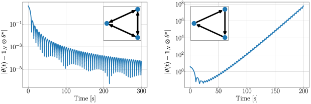
Consider a multi-agent system with three agents, i.e., 𝒱={1,2,3}\mathcal{V}=\{1,2,3\}. We let kt=0k_{t}=0 and di=0d_{i}=0, and for simplicity we assume that all agents use the same coefficient τc=τ1=τ2=τ3\tau_{c}=\tau_{1}=\tau_{2}=\tau_{3}, with τ(0)=0\tau(0)=0 and ω=1/2\omega=1/2. We consider regressors ϕi(t)=(1,10eit,100e2it)\phi_{i}(t)=(1,10e^{-it},100e^{-2it}) with collected data satisfying Assumption 1, and the parameter θ=(1,2,1)\theta^{\star}=(1,-2,1). The DMCL dynamics are implemented using τ˙c=1/2\dot{\tau}_{c}=1/2. The left plot of Figure 1 shows the evolution in time (in logarithmic scale) of the estimation error θ~=θ𝟏Nθ\tilde{\theta}=\theta-\mathbf{1}_{N}\otimes\theta^{\star} when the graph 𝒢\mathcal{G} is fully connected. As observed, the estimation error converges to zero, which is consistent with the stability results of [13, Thm. 3] and the fact that in this case, the DMCL dynamics describe an accelerated gradient system. Now, suppose that the communication graph is given by a directed cycle graph, as shown on the inset of the right plot of Figure 1. In this case, the same DMCL algorithm ceases to be a momentum-based gradient flow and it exhibits the instability issue shown in the plot. The right plot, however, reveals a promising solution to the instability issue in asymmetric graphs. Stability can be restored by implementing a well-designed restart mechanism that accounts for the graph’s asymmetry. The details of this mechanism will be elaborated upon in the following sections. \square

3.3 DMCL with Coordinated Restart

To address the instability observed in Example 1, while simultaneously inducing suitable convergence rates achieved via momentum, we can incorporate restart mechanisms into the algorithm. Such mechanisms persistently reset the momentum θ˙i\dot{\theta}_{i} and the dynamic coefficients τi\tau_{i} whenever τi\tau_{i} exceeds the upper bound TT. The resets are performed according to the following discrete-time updates:

θi+=θi,pi+=pi+ηi(θipi),τi+=T0,i𝒱,\theta_{i}^{+}=\theta_{i},~{}~{}~{}p_{i}^{+}=p_{i}+\eta_{i}(\theta_{i}-p_{i}),~{}~{}~{}\tau_{i}^{+}=T_{0},~{}~{}~{}\forall~{}i\in\mathcal{V}, (15)

where ηi{0,1}\eta_{i}\in\{0,1\} is a pre-defined parameter indicating the restart policy of agent ii. It has been shown that this approach can curtail the oscillations of momentum-based algorithms [13, 17] and also “robustify” their stability properties with respect to persistent disturbances [19]. Indeed, note that the policy ηi=1\eta_{i}=1 implies pi+=θip_{i}^{+}=\theta_{i}, which implies θ˙i+=0\dot{\theta}_{i}^{+}=0. For multi-agent systems with undirected graphs, similar restart mechanisms of the form (15) have been studied in [25, 24]. However, the effectiveness of restarting in the context of multi-agent systems with directed graphs has remained largely unexplored, and, as suggested by Example 1 the extension is non-trivial. Indeed, from the behavior observed in Figure 1 it should be clear that a “slow” restart policy (e.g., when TT is large) will not be able to stabilize the system. However, a “fast” restart policy (e.g., when TT is small) would keep pip_{i} approximately constant, thus reducing the effectiveness of using momentum. The right plot of Figure 1 shows the emerging behavior of the DMCL algorithm when restart is implemented by each node of the network with a “suitable” frequency and in a coordinated manner. While similar phenomena has been recently observed in game-theoretic problems [24], the use of momentum and restart in decentralized CL problems, and its dependence on the data of the system, the topology of the graph, and the perturbed models (3) have remained largely unexplored. This observation motivates the main research problem that we study in this paper:

Problem 1

Characterize the restart mechanisms that: a) robustly stabilize the DMCL algorithm in directed networks; b) achieve ISS with respect to the disturbances did_{i} in (3); c) induce network-wide acceleration properties in the MAS. \square

In the next section we provide an answer to Problem 1 using tools from hybrid dynamical systems and graph theory.

4 Main Results

To tackle Problem 1, we first consider a centralized restart mechanism that makes use of a common state τc>0\tau_{c}\in\mathbb{R}_{>0} that satisfies τ˙c[0,ω]\dot{\tau}_{c}\in[0,\omega]. This centralized assumption simplifies the analysis and will be relaxed in the subsequent subsections to encompass decentralized implementations. For the purpose of analysis, we also use an auxiliary state ss\in\mathbb{R} with dynamics s˙=1\dot{s}=1 to model any explicit dependence on time tt.

4.1 Centralized Restart: Hybrid Systems Model

When using a common coefficient τc>0\tau_{c}\in\mathbb{R}_{>0} to coordinate the restart of the DMCL algorithm, the resulting dynamical system can be modeled by the following differential inclusion, in vectorial form, with state yc(θ,p,τc,s)y_{c}\coloneqq(\theta,p,\tau_{c},s):

y˙c𝐅c(yc,u)(2τc(pθ)2τc𝚲(θ,s,u)[0,ω]1),\displaystyle\dot{y}_{c}\!\in\!\mathbf{F}_{c}(y_{c},u)\coloneqq\begin{pmatrix}\dfrac{2}{\tau_{c}}(p-\theta)\\ \!-2\tau_{c}\mathbf{\Lambda}(\theta,s,u)\!\\ [0,\omega]\\ 1\end{pmatrix}, (16)

whenever yc𝐂c×0y_{c}\in\mathbf{C}_{c}\times\mathbb{R}_{\geq 0}, and where u(υ,ν)u\coloneqq(\upsilon,\nu), the function 𝚲\mathbf{\Lambda} is given by

𝚲(θ,s,u)kt𝚿(θ,s,υ)+kr𝚽(θ,ν)+kc𝐋θ,\mathbf{\Lambda}(\theta,s,u)\coloneqq k_{t}\mathbf{\Psi}(\theta,s,\upsilon)+k_{r}\mathbf{\Phi}(\theta,\nu)+k_{c}\mathbf{L}\theta, (17)

and the vectors υ\upsilon and ν\nu are defined as

υ(υ1,υ2,,υN)N,ν(ν1,ν2,,νN)k¯,\displaystyle\upsilon\coloneqq(\upsilon_{1},\upsilon_{2},\dots,\upsilon_{N})\in\mathbb{R}^{N},~{}~{}~{}\nu\coloneqq(\nu_{1},\nu_{2},\dots,\nu_{N})\in\mathbb{R}^{\bar{k}},

where k¯:=i𝒱k¯i\bar{k}:=\sum_{i\in\mathcal{V}}\overline{k}_{i}. The maps 𝚿\mathbf{\Psi} and 𝚽\mathbf{\Phi} above are defined as

𝚿(θ,s,υ)\displaystyle\!\!\!\!\!\!\!\mathbf{\Psi}(\theta,s,\upsilon) (Ψ1(θ1,s,υ1),,ΨN(θN,s,υN))\displaystyle\coloneqq(\Psi_{1}(\theta_{1},s,\upsilon_{1}),\dots,\Psi_{N}(\theta_{N},s,\upsilon_{N})) (18a)
𝚽(θ,ν)\displaystyle\mathbf{\Phi}(\theta,\nu) (Φ1(θ1,ν1),,ΦN(θN,νN)),\displaystyle\coloneqq(\Phi_{1}(\theta_{1},\nu_{1}),\dots,\Phi_{N}(\theta_{N},\nu_{N})), (18b)

where the functions Φi,Ψi\Phi_{i},\Psi_{i} were defined in (5)-(6) for all i𝒱i\in\mathcal{V}. Since θ\theta and pp are allowed to evolve in nN\mathbb{R}^{nN}, while τc[T0,T]\tau_{c}\in[T_{0},T], in (16), the flow set 𝐂c\mathbf{C}_{c} is defined as:

𝐂cnN×nN×[T0,T],\mathbf{C}_{c}\coloneqq\mathbb{R}^{nN}\times\mathbb{R}^{nN}\times[T_{0},T], (19)

which guarantees that during flows the state τc\tau_{c} remains in the interval [T0,T][T_{0},T]. To incorporate restarts into the DMCL algorithm, each time τc\tau_{c} meets the condition τc=T\tau_{c}=T, it is reset to T0T_{0}, and, all the states (θi,pi)(\theta_{i},p_{i}) are updated as in (15). Therefore, using

𝐑ηdiag(η)In,\mathbf{R}_{\eta}\coloneqq\text{diag}(\eta)\otimes I_{n}, (20)

with η=(η1,η2,,ηN)\eta=(\eta_{1},\eta_{2},\ldots,\eta_{N}), the discrete-time updates of the states (θ,p,τ)(\theta,p,\tau) of the hybrid system can be written in vectorial form as

(θ+,p+,τc+)=𝐆^c(xc)=(θ,p+𝐑η(θp),T0)\displaystyle\!\!\!(\theta^{+},p^{+},\tau_{c}^{+})=\hat{\mathbf{G}}_{c}(x_{c})=(\theta,p+\mathbf{R}_{\eta}(\theta{-}p),T_{0}) (21)

which are executed whenever (θ,p,τ)(\theta,p,\tau) are in the jump set 𝐃c\mathbf{D}_{c}, defined as follows:

𝐃cnN×nN×{T}.\mathbf{D}_{c}\coloneqq\mathbb{R}^{nN}\times\mathbb{R}^{nN}\times\{T\}. (22)

Therefore, the overall discrete-time dynamics of the system with state ycy_{c} can be written as:

yc𝐃c×0,yc+=𝐆c(yc)𝐆^c(yc)×{s}.\displaystyle y_{c}\in\mathbf{D}_{c}\times\mathbb{R}_{\geq 0},\quad y_{c}^{+}=\mathbf{G}_{c}(y_{c})\coloneqq\hat{\mathbf{G}}_{c}(y_{c})\!\times\!\{s\}. (23)

By combining (16) and (23), the DMCL algorithm with centralized restart can be viewed as a HDS of the form (1), with data

c(𝐂c×0,𝐅c,𝐃c×0,𝐆c).\mathcal{H}_{c}\coloneqq(\mathbf{C}_{c}\times\mathbb{R}_{\geq 0},\mathbf{F}_{c},\mathbf{D}_{c}\times\mathbb{R}_{\geq 0},\mathbf{G}_{c}). (24)

Note that in this centralized HDS the jump set (22) only imposes conditions on the state τc\tau_{c}. Namely, a restart is triggered whenever τc=T\tau_{c}=T. If τ˙(t)=constant[0,ω]\dot{\tau}(t)=\text{constant}\in[0,\omega] for all time, then the HDS would model a DMCL algorithm with scheduled periodic restart, where the time between two consecutive restarts is (TT0)ω1(T-T_{0})\omega^{-1}. However, the differential inclusion in (16) also allows us to consider scenarios where τ˙\dot{\tau} is not constant but rather is any absolutely continuous function (between restarts) satisfying τ˙[0,ω]\dot{\tau}\in[0,\omega], which includes functions that remain constant for arbitrarily long periods of time.

Before presenting our first main result, we introduce two technical propositions that play important roles in our results. All the proofs are presented in Section 6.

Proposition 1

Suppose that Assumption 1 holds. Then, there exists a unit vector qNq\in\mathbb{R}^{N} such that:

  1. (a)

    The entries qiq_{i} of qq satisfy:

    σ¯𝐐maxi𝒱qimini𝒱qi:=σ¯𝐐>0.\displaystyle\overline{\sigma}_{\mathbf{Q}}\coloneqq\max_{i\in\mathcal{V}}q_{i}\geq\min_{i\in\mathcal{V}}q_{i}:=\underline{\sigma}_{\mathbf{Q}}>0. (25)
  2. (b)

    q=0q^{\top}\mathcal{L}=0 and 𝒬+𝒬0\mathcal{Q}\mathcal{L}+\mathcal{L}^{\top}\mathcal{Q}\succeq 0 with 𝒬diag(q)\mathcal{Q}\coloneqq\text{diag}(q).

  3. (c)

    The function 𝚲(θ,s,u)\mathbf{\Lambda}(\theta,s,u) in (17) with kt=0k_{t}=0 and ν=0\nu=0 can be decomposed as follows:

    kr𝚽(θ,0)+kc𝐋θ=𝐐1(𝚺+𝛀)θ~,\displaystyle k_{r}\mathbf{\Phi}(\theta,0)+k_{c}\mathbf{L}\theta=\mathbf{Q}^{-1}\left(\mathbf{\Sigma}+\mathbf{\Omega}\right)\tilde{\theta}, (26)

    where 𝐐𝒬In\mathbf{Q}\coloneqq\mathcal{Q}\otimes I_{n}, θ~:=θ𝟏Nθ\tilde{\theta}:=\theta-\mathbf{1}_{N}\otimes\theta^{\star},

    𝚺\displaystyle\mathbf{\Sigma} :=kr𝐐𝚫+kc2(QL+LQ)\displaystyle:=k_{r}\mathbf{Q}\mathbf{\Delta}\!+\!\frac{k_{\text{c}}}{2}\left(\textbf{Q}\textbf{L}\!+\!\textbf{L}^{\top}\textbf{Q}\right) (27a)
    𝛀\displaystyle\mathbf{\Omega} :=kc2(QLLQ),\displaystyle:=\!\frac{k_{\text{c}}}{2}\left(\textbf{Q}\textbf{L}\!-\!\textbf{L}^{\top}\textbf{Q}\right), (27b)

    and 𝚫diag({Δ1,Δ2,,ΔN})\mathbf{\Delta}\coloneqq\textbf{diag}\left(\{\Delta_{1},\Delta_{2},\dots,\Delta_{N}\}\right), where Δi\Delta_{i} is given by (7).

  4. (d)

    There exists a class-𝒦\mathcal{K}_{\infty} function χ()\chi(\cdot) such that

    [𝛀+kt𝐀~(t)][𝛀+kt𝐀~(t)](σ¯𝛀2+χ(kt)2)INn,\displaystyle\!\!\!\!\Bigl{[}\mathbf{\Omega}+k_{t}\tilde{\mathbf{A}}(t)\biggr{]}\biggl{[}\mathbf{\Omega}+k_{t}\tilde{\mathbf{A}}(t)\Bigr{]}^{\!\!\top}\!\!\!\preceq(\overline{\sigma}_{\mathbf{\Omega}}^{2}+\chi(k_{t})^{2})I_{Nn}, (28)

    t0\forall~{}t\geq 0, where 𝐀~(t)𝐐𝐀(t)\tilde{\mathbf{A}}(t)\coloneqq\mathbf{Q}\mathbf{A}(t) and σ¯𝛀\overline{\sigma}_{\mathbf{\Omega}} is the largest singular value of 𝛀\mathbf{\Omega}. \square

Remark 2

By construction, if the Laplacian \mathcal{L} is symmetric, then σ¯𝛀2=0\overline{\sigma}_{\mathbf{\Omega}}^{2}=0. However, if \mathcal{L} is asymmetric, then in general we have σ¯𝛀20\overline{\sigma}_{\mathbf{\Omega}}^{2}\neq 0. For the purpose of illustration, Figure 2 presents four examples of different graphs 𝒢\mathcal{G} and their corresponding numerical values of σ¯𝛀2\overline{\sigma}_{\mathbf{\Omega}}^{2}. \square

Proposition 2

Suppose that Assumption 1 holds; then, there exist σ¯𝚺σ¯𝚺>0\overline{\sigma}_{\mathbf{\Sigma}}\geq\underline{\sigma}_{\mathbf{\Sigma}}>0 such that

σ¯𝚺INn𝚺σ¯𝚺INn,\overline{\sigma}_{\mathbf{\Sigma}}I_{Nn}\succeq\mathbf{\Sigma}\succeq\underline{\sigma}_{\mathbf{\Sigma}}I_{Nn}, (29)

where 𝚺\mathbf{\Sigma} is given by (27). \square

4.2 Input-to-State Stability of c\mathcal{H}_{c}

Refer to caption
Figure 2: Parameter σ¯𝛀2\overline{\sigma}_{\mathbf{\Omega}}^{2} for strongly connected graphs with binary adjacency matrices and varying degrees of symmetry.

With Propositions 1-2 at hand, we are now ready to present the first main result of this paper, which provides conditions to stabilize the DMCL algorithm using a centralized restart. In particular, we study the stability properties of c\mathcal{H}_{c} with respect to the closed set 𝒜c𝒜θp×[T0,T]×0\mathcal{A}_{c}\coloneqq\mathcal{A}_{\theta p}\times[T_{0},T]\times\mathbb{R}_{\geq 0}, where

𝒜θp{𝟏Nθ}×{𝟏Nθ},\displaystyle\mathcal{A}_{\theta p}\coloneqq\{\mathbf{1}_{N}\otimes\theta^{\star}\}\times\{\mathbf{1}_{N}\otimes\theta^{\star}\}, (30)

which precisely describes the situation where all agent’s estimates θi\theta_{i} are equal to the true parameter θ\theta^{*}.

Theorem 1

Suppose that Assumption 1 holds, and let the constants (σ¯𝐐\underline{\sigma}_{\mathbf{Q}}, σ¯𝐐\overline{\sigma}_{\mathbf{Q}}, σ¯𝛀2\overline{\sigma}_{\mathbf{\Omega}}^{2}, σ¯𝚺\underline{\sigma}_{\mathbf{\Sigma}}) be given by Proposition 1. If the restart parameters (ω,T0,T)(\omega,T_{0},T) satisfy ω(0,1)\omega\in(0,1) and

(12σ¯𝐐σ¯𝚺+T02)12𝐓¯<T<𝐓¯(σ¯𝐐(1ω)σ¯𝚺σ¯𝛀2+χ(kt)2)12,\displaystyle\left(\frac{1}{2}\frac{\overline{\sigma}_{\mathbf{Q}}}{\underline{\sigma}_{\mathbf{\Sigma}}}{+}{T_{0}^{2}}\right)^{\frac{1}{2}}\eqqcolon\underline{\mathbf{T}}<T<\overline{\mathbf{T}}\coloneqq\!\left(\frac{\underline{\sigma}_{\mathbf{Q}}(1-\!\omega)\underline{\sigma}_{\mathbf{\Sigma}}}{{\overline{\sigma}^{2}_{\mathbf{\Omega}}+\chi(k_{t})^{2}}}\right)^{\frac{1}{2}}, (31)

then the following hold:

  1. (a)

    For any restart policy η{0,1}N\eta\in\{0,1\}^{N} the HDS c\mathcal{H}_{c} renders the set 𝒜c\mathcal{A}_{c} ISS with respect to the input uu.

  2. (b)

    If ηi=1\eta_{i}=1 for all i𝒱i\in\mathcal{V}, and τ˙cω\dot{\tau}_{c}\coloneqq\omega, then, for every initial condition y0:=yc(0,0)(𝐂c𝐃c)×0y_{0}:=y_{c}(0,0)\in(\mathbf{C}_{c}\cup\mathbf{D}_{c})\times\mathbb{R}_{\geq 0}, every solution-input pair (yc,u)(y_{c},u) of c\mathcal{H}_{c}, and every (tj,j)dom(yc,u)(t_{j},j)\in\text{dom}(y_{c},u) with tjmin{t:(t,j)dom(yc,u)}t_{j}\coloneqq\min\{t:(t,j)\in\text{dom}(y_{c},u)\}, the sampled sequence of estimates θ(tj,j)\theta(t_{j},j) satisfies

    |θ(tj,j)𝟏Nθ|2k1μj|y0|𝒜c2+k2|u|(tj,j)2,|\theta(t_{j},j)-\mathbf{1}_{N}\otimes\theta^{\star}|^{2}\leq k_{1}\cdot\mu^{j}|y_{0}|_{\mathcal{A}_{c}}^{2}+k_{2}|u|^{2}_{(t_{j},j)}, (32)

    where k1,k2>0k_{1},k_{2}>0, and μ(T)(𝐓¯/T)2\mu(T)\coloneqq(\underline{\mathbf{T}}/T)^{2}. \square

The main result of Theorem 1 reveals the impact of the asymmetry of 𝒢\mathcal{G} on the resetting parameter TT. In particular, the following observations are in order:

(1) When \mathcal{L} is symmetric (i.e., σ¯𝛀2=0\overline{\sigma}_{\mathbf{\Omega}}^{2}=0) and the DMCL dynamics do not use real-time data (i.e., kt=0k_{t}=0), condition (31) reduces to 𝐓¯<T<\underline{\mathbf{T}}<T<\infty, which can always be satisfied using any positive constant TT, recovering the results of [19, Thm. 2] in the context of optimization.

(2) In general, the more “informative” is the collective data in the overall system (i.e., the larger is α\alpha in (8)), the larger the parameter σ¯𝚺\underline{\sigma}_{\mathbf{\Sigma}} will be, thus providing more flexibility to increase the upper bound TT.

(3) The ISS result implies that the trajectories of the algorithm will converge to a neighborhood of the true parameter θ\theta^{\star}, where the size of the neighborhood shrinks as the disturbances did_{i} shrink in (3). When di=0d_{i}=0, the result establishes asymptotic convergence to the true parameter.

(4) Lastly, when u0u\equiv 0, the bound (32) characterizes the “accelerated” convergence properties of c\mathcal{H}_{c} towards the true model θ\theta^{\star}. Since the rate of convergence is TT-dependent, the rate of convergence depends on TT. In particular, following similar steps as in the centralized case [19], the “optimal” value of TT that minimizes the contraction coefficient μ(T)\mu(T) over a given window of time can be computed as T=e(σ¯𝐐2σ¯𝚺+T02)12T^{*}=e\left(\frac{\overline{\sigma}_{\mathbf{Q}}}{2\underline{\sigma}_{\mathbf{\Sigma}}}+{T_{0}^{2}}\right)^{\frac{1}{2}}.

Next, the following corollary leverages the expression of TT^{*} to obtain convergence bounds that parallel those obtained for centralized single-agent systems [19].

Corollary 1

Suppose that all the assumptions of Theorem 1 hold with T=TT=T^{*}, τ˙c=ω\dot{\tau}_{c}=\omega and u0u\equiv 0; then, (32) holds with k2=0k_{2}=0, and for each ε>0\varepsilon>0 we have |θ(tj,j)𝟏Nθ|2ε|\theta(t_{j},j)-\mathbf{1}_{N}\otimes\theta^{\star}|^{2}\leq\varepsilon for all tj>tjt_{j}>t_{j}^{*}, where tj12ω(TT0)log(1εc¯c¯|y0|𝒜2).t_{j}^{*}\coloneqq\frac{1}{2\omega}\left(T^{*}-T_{0}\right)\log\left(\frac{1}{\varepsilon}\frac{\overline{c}}{\underline{c}}|y_{0}|_{\mathcal{A}}^{2}\right). \square

The bound from Corollary 1 implies that, as T00+T_{0}{\to}0^{+}, the convergence of θi\theta_{i} towards θi\theta_{i}^{*} is of order 𝒪(eσ¯𝚺/σ¯𝐐)\mathcal{O}\left({e^{-\sqrt{\underline{\sigma}_{\mathbf{\Sigma}}/\overline{\sigma}_{\mathbf{Q}}}}}\right), for all i𝒱i\in\mathcal{V}. We complete this section with a corollary for the case η=0\eta=0, which guarantees the ISS properties of c\mathcal{H}_{c}, but not convergence bounds of the form (32).

Corollary 2

Suppose that Assumption 1 holds, ηi=0\eta_{i}=0 for all i𝒱i\in\mathcal{V}, ω(0,1)\omega\in(0,1), and T0<T<𝐓¯T_{0}<T<\overline{\mathbf{T}}, with 𝐓¯\overline{\mathbf{T}} as defined in (31). Then, the HDS c\mathcal{H}_{c} renders the set 𝒜c\mathcal{A}_{c} ISS. \square

The resetting bounds of Theorem 1 and Corollary 2 only provide sufficient conditions for ISS with exponential convergence rates. It remains an open question how to obtain tight bounds on (T0,T)(T_{0},T) that are also necessary for stability. We do not further pursue these questions in this paper.

4.3 Decentralized Restart: Synchronization

Since a central coordinator might not exist in large-scale networks, in this section, we study decentralized restart strategies based on each agent i𝒱i\in\mathcal{V} implementing an individual dynamic coefficient τi\tau_{i}. To simplify our discussion, in this section we assume that ηi=1\eta_{i}=1 and τ˙i=ω\dot{\tau}_{i}=\omega for all i𝒱i\in\mathcal{V}, and that kt=0k_{t}=0, which allows us to remove the state variable ss and its associated dynamics. However, all our results can be extended to the case when time-varying regressors are included.

When each agent implements its own coefficient τi\tau_{i}, the continuous-time DMCL dynamics (16) become

x𝐂,x˙=𝐅(x,u)(2𝒯1(pθ)2𝒯(kr𝚽(θ,u)+kc𝐋θ)ω𝟏N),x\in\mathbf{C},~{}~{}\dot{x}=\mathbf{F}(x,u)\coloneqq\begin{pmatrix}2\mathcal{T}^{-1}(p-\theta)\\ -2\mathcal{T}(k_{r}\mathbf{\Phi}(\theta,u)+k_{c}\mathbf{L}\theta)\\ \omega\mathbf{1}_{N}\end{pmatrix}, (33)

where the main state is now x=(θ,p,τ)Nn×Nn×Nx=(\theta,p,\tau)\in\mathbb{R}^{Nn}\times\mathbb{R}^{Nn}\times\mathbb{R}^{N}, 𝒯diag(τ𝟏n)\mathcal{T}\coloneqq\text{diag}(\tau\otimes\mathbf{1}_{n}), τ=(τ1,τ2,,τN)\tau=(\tau_{1},\tau_{2},\dots,\tau_{N}), 𝚽\mathbf{\Phi} is given by (18b), and the flow set is given by

𝐂N×N×[T0,T]N.\mathbf{C}\coloneqq\mathbb{R}^{N}\times\mathbb{R}^{N}\times[T_{0},T]^{N}. (34)

In this case, restarts of the form (15) with ηi=1\eta_{i}=1 occur whenever at least one of the agents satisfies the condition τi=T\tau_{i}=T. This behavior can be modeled by the following jump set:

𝐃={x𝐂:maxi𝒱τi=T}.\mathbf{D}=\left\{x\in\mathbf{C}:~{}\max_{i\in\mathcal{V}}\tau_{i}=T\right\}. (35)

However, note that this approach would lead to uncoordinated restarts of the individual dynamics of the agents across the system. For example, for any time window [T0,T][T_{0},T], one can select NN equidistant initial conditions τi(0,0)[T0,T]\tau_{i}(0,0)\in[T_{0},T], where i{1,2,,N}i\in\{1,2,\ldots,N\}, which result in solutions experiencing NN restarts during this time window, each restart separated by intervals of flow of length TT0N\frac{T-T_{0}}{N}. Therefore, as NN\to\infty, asynchronous restarts would occur more often, hindering the advantages of incorporating momentum into the flows of the algorithm to accelerate the overall system.

To address this issue, and inspired by the synchronization algorithms of [36], we integrate the restart dynamics (15) of each agent with a decentralized coordination mechanism for the states τi\tau_{i}. Specifically, each agent i𝒱i\in\mathcal{V} performs individual restarts of the form (15) when τi=T\tau_{i}=T. However, the agents also implement the following additional discrete-time updates whenever their neighbors j𝒩ij\in\mathcal{N}_{i} satisfy the condition τj=T\tau_{j}=T:

τi+i(τi){T0ifτi[T0,ri){T0,T}ifτi=riTifτi(ri,T],\tau_{i}^{+}\in\mathcal{R}_{i}(\tau_{i})\coloneqq\left\{\begin{array}[]{cl}T_{0}&\text{if}~{}\tau_{i}\in[T_{0},r_{i})\\ \{T_{0},T\}&\text{if}~{}~{}\tau_{i}=r_{i}\\ T&\text{if}~{}\tau_{i}\in(r_{i},T]\end{array}\right., (36)

where ri>0r_{i}>0 is a tunable parameter. To incorporate these additional discrete-time updates into the overall jump map of the system, consider the set-valued map

Gd(x){(θ^,p^,τ^)\displaystyle G_{d}(x)\coloneqq\Big{\{}(\hat{\theta},\hat{p},\hat{\tau})\in (2n+1)N:θ^=θ,p^i=pi,τ^i=T0,\displaystyle~{}\mathbb{R}^{(2n+1)N}:\hat{\theta}=\theta,~{}\hat{p}_{i}=p_{i},~{}\hat{\tau}_{i}=T_{0},
τjj(τj),p^j=pj,j𝒩i,\displaystyle\tau_{j}\in\mathcal{R}_{j}(\tau_{j}),~{}\hat{p}_{j}=p_{j},~{}\forall j\in\mathcal{N}_{i},
p^k=pk,τ^k=τkkij},\displaystyle\hat{p}_{k}=p_{k},~{}\hat{\tau}_{k}=\tau_{k}~{}\forall k\neq i\neq j\Big{\}},

which is defined to be non-empty if and only if τi=T\tau_{i}=T and τj[0,T)\tau_{j}\in[0,T). In words, the mapping Gd(x)G_{d}(x) captures the resets of the individual states (θi,pi,τi)2n+1(\theta_{i},p_{i},\tau_{i})\in\mathbb{R}^{2n+1} of agent ii via (15), and also the updates of its neighbors j𝒩ij\in\mathcal{N}_{i} via (36). The overall jump-map of the multi-agent hybrid system can then be defined using the outer-semicontinuous hull of GdG_{d}111The outer-semicontinuous hull of a set-valued mapping G:nnG:\mathbb{R}^{n}\rightrightarrows\mathbb{R}^{n} is the unique set-valued mapping G¯:nn\bar{G}:\mathbb{R}^{n}\rightrightarrows\mathbb{R}^{n} satisfying graph(G¯)=cl(graph(G))\text{graph}(\bar{G})=\text{cl}(\text{graph}(G)), where cl()\text{cl}(\cdot) stands for the closure., denoted G¯d\overline{G}_{d} leading to

x𝐃,x+𝐆(x)G¯d(x).x\in\mathbf{D},~{}~{}~{}x^{+}\in\mathbf{G}(x)\coloneqq\overline{G}_{d}(x). (37)

Note that system (37) preserves the sparsity property of the graph 𝒢\mathcal{G}.

The decentralized continuous-time dynamics (33) and the decentralized discrete-time dynamics (37) comprise the overall DMCL algorithm with restarts studied in this paper. This algorithm is fully modeled by the HDS

(𝐂,𝐅,𝐃,𝐆)\mathcal{H}\coloneqq(\mathbf{C},\mathbf{F},\mathbf{D},\mathbf{G}) (38)

with state x=(θ,p,τ)Nn×Nn×Nx=(\theta,p,\tau)\in\mathbb{R}^{Nn}\times\mathbb{R}^{Nn}\times\mathbb{R}^{N}.

The following theorem provides a decentralized version of Theorem 1. In this case, stability of τ\tau is studied with respect to the “synchronized” set 𝒜sync[T0,T]𝟏N{T0,T}N\mathcal{A}_{\text{sync}}\coloneqq[T_{0},T]\cdot\mathbf{1}_{N}\cup\{T_{0},T\}^{N}, and the stability properties of the overall state are studied with respect to

𝒜𝒜θp×𝒜sync.\mathcal{A}\coloneqq\mathcal{A}_{\theta p}\times\mathcal{A}_{\text{sync}}. (39)

For simplicity, we state the result for the case u=0u=0, but we comment on the robustness properties of the dynamics.

Theorem 2

Consider the HDS \mathcal{H} and suppose that Assumption 1 holds and that:

  1. (a)

    The parameters (T0,T)(T_{0},T) satisfy (31).

  2. (b)

    The constants {ri}i𝒱\{r_{i}\}_{i\in\mathcal{V}} satisfy T0<ri<T0+(TT0)N1T_{0}<r_{i}<T_{0}+\frac{(T-T_{0})}{N-1}

Then, the set 𝒜𝒜θp×𝒜sync\mathcal{A}\coloneqq\mathcal{A}_{\theta p}\times\mathcal{A}_{\text{sync}} is UGES for \mathcal{H}, and there exists a time t[0,2TT0ω)t^{*}\in\left[0,2\frac{T-T_{0}}{\omega}\right) such that for every solution xx of \mathcal{H} and every (t,j)dom(y)(t,j)\in\text{dom}(y) such that t+jt+2Nt+j\geq t^{*}+2N, the bound (32) holds. \square

Refer to caption
Refer to caption
Figure 3: Left: Trajectories of \mathcal{H} when 𝒢\mathcal{G} is fully connected. Right: Trajectories of \mathcal{H} when 𝒢\mathcal{G} is a cycle. Here, θ~=θ𝟏Nθ\tilde{\theta}=\theta-\mathbf{1}_{N}\otimes\theta^{\star}
Remark 3 (Nominal Robustness)

Since the hybrid system \mathcal{H} is nominally well-posed in the sense of [29, Ch. 6], the UGES properties of the DMCL algorithm are preserved, in a semi-global practical sense, under arbitrarily small additive perturbations on states and dynamics. This property is crucial for the use of \mathcal{H} in practical applications where dynamic disturbances are unavoidable. \square

Remark 4 (Strong Robustness via ISS)

The techniques employed to proof Theorem 2 can be further utilized to obtain ISS of \mathcal{H} provided that uu originates from a dynamical system evolving in a compact set. We omit this extension due to space constraints. \square

Remark 5

Since system \mathcal{H} has no finite-escape times due to the global Lipschitz property of 𝐅\mathbf{F} in 𝐂\mathbf{C}, it follows that the stability results of Corollary 2 also extend to \mathcal{H} with ηi=0\eta_{i}=0 for all ii, recovering the convergence result of Theorem 1 after an initial finite synchronization phase. \square

To the best of the author’s knowledge, Theorems 1-2 and the respective corollaries, are the first stability results for momentum-based CL algorithms implemented in multi-agent systems with general directed graphs. We note that in the literature of centralized CL, other accelerated algorithms have been studied using finite-time and fixed-time stability tools [3, 37, 38]. However, as shown in the comparison presented in [3], when the “level of richness” of the data (i.e., α\alpha in Assumption 1) is “low”, momentum-based methods can yield better transient performance compared to other first-order non-smooth techniques. For decentralized problems defined over networks, we are not aware of finite-time or fixed-time CL algorithms that are stable under Assumption 8. A natural progression for future research involves developing such algorithms and comparing them with the DMCL algorithms proposed in this paper.

5 Applications in Estimation, Control, and Model-free Feedback Optimization

In this section, we apply the DMCL algorithm with restart in three different applications.

5.1 Hybrid Cooperative Identification Over Digraphs

First, we validate Theorem 2 in an cooperative estimation problem defined in a multi-agent system with N=5N=5, n=3n=3, and ψi(s)=(10eis1)2\psi_{i}(s)=(10e^{-is}-1)^{2}, for all i𝒱i\in\mathcal{V}. To implement the DMCL algorithm with coordinated restarts, we parameterize ψi()\psi_{i}(\cdot) using the regressor ϕi(s)(1,10eis,100e2is)\phi_{i}(s)\coloneqq(1,10e^{-is},100e^{-2is}) and θ=(1,2,1)\theta^{\star}=(1,-2,1). To satisfy Assumption 1 with α=5.5\alpha=5.5, each agent records five measurements of ψi\psi_{i}. We implement the hybrid system \mathcal{H} and plot the resulting trajectories of the estimation error in the left plot of Figure 3, using kr=80,kc=0.08k_{r}=80,k_{c}=0.08, and a fully connected graph. We also show with dashed lines the trajectory obtained when using the first-order decentralized CL dynamics of [7]. Since the graph is symmetric, in this case TT can be selected arbitrarily large to tune the convergence rate of the dynamics (see inequality (31)). The simulations start from a non-synchronized initial condition τ(0,0)τ0𝟏5\tau(0,0)\neq\tau_{0}\mathbf{1}_{5} and rapidly achieve synchronization. Trajectories related to different choices of TT are also shown to illustrate the impact of the restart period on the convergence rate. Next, we let 𝒢\mathcal{G} be a cycle digraph, for which σ¯𝛀2=0.18\overline{\sigma}_{\mathbf{\Omega}}^{2}=0.18. The resetting parameter TT is selected to satisfy inequality (31), and the resulting trajectories are shown in the right plot of Figure 3. In this case, the best transient performance is obtained as TT approaches the upper bound 𝐓¯\overline{\mathbf{T}}.

5.2 Data-Enabled Hybrid Cooperative MRAC

A key advantage of the robust stability results presented in Theorems 1 and 2, is that the DMCL dynamics can be interconnected with other systems for the solution of feedback control problems. To illustrate this application, we consider a multi-agent dynamical system, where each agent has individual dynamics of the form:

χ˙i=Aiχi+Biui+Biψ~i(θ,χi),χin,uim,\dot{\chi}_{i}=A_{i}\chi_{i}+B_{i}u_{i}+B_{i}\tilde{\psi}_{i}(\theta^{\star},\chi_{i}),~{}~{}\chi_{i}\in\mathbb{R}^{n},~{}u_{i}\in\mathbb{R}^{m}, (40)

where ψ~i(θ,χ)=ϕi(χ)θ\tilde{\psi}_{i}(\theta^{\star},\chi)=\phi_{i}\left(\chi\right)^{\top}\theta^{\star} models structured uncertainty parameterized by a common vector θ\theta^{\star}, and a regressor ϕi\phi_{i} that is known by each agent ii. The agent’s goal is to be able to asymptotically track a common bounded reference rr despite the uncertainty in their model.

Refer to caption
Refer to caption
Figure 4: Left: Scheme of the ithi^{th} agent’s dynamics in the Cooperative MRAC. 𝐅i\mathbf{F}_{i} and 𝐆i\mathbf{G}_{i} represent the components of the overall DMCL flow-map and jump-map, respectively, corresponding to the state xi=(θi,pi,τi)2n+1x_{i}=(\theta_{i},p_{i},\tau_{i})\in\mathbb{R}^{2n+1}. Right: Trajectories resulting from the Cooperative MRAC when N=5N=5.

5.2.1 Two-Time Scale Hybrid Dynamics

To solve the tracking problem we use a two-time scale approach. First, we introduce a reference model χ˙r=Arχr+Brr\dot{\chi}_{r}=A_{r}\chi_{r}+B_{r}r, where ArA_{r} is assumed to be Hurwitz. Following the ideas of [9], each agent implements a model-reference adaptive control (MRAC) law that incorporates three elements: (1) an adaptive component uai(θi,χi)=ϕi(χi)θiu_{a_{i}}(\theta_{i},\chi_{i})=\phi_{i}(\chi_{i})^{\top}\theta_{i}, where θi\theta_{i} is the individual estimate of θ\theta^{\star}; (2) a state-feedback component usi(χi,χr)=K(χiχr)u_{s_{i}}(\chi_{i},\chi_{r})=-K(\chi_{i}-\chi_{r}); and (3) a feed-forward term ufiu_{f_{i}} designed such that Biufi(χr)=(ArAi)χr+BrrB_{i}u_{f_{i}}(\chi_{r})=(A_{r}-A_{i})\chi_{r}+B_{r}r; see Figure 4 for an illustration of the control law. Using ui(θi,χi,χr)=usi(χi,χr)+ufi(χr)uai(θi,χi)u_{i}(\theta_{i},\chi_{i},\chi_{r})=u_{s_{i}}(\chi_{i},\chi_{r})+u_{f_{i}}(\chi_{r})-u_{a_{i}}(\theta_{i},\chi_{i}), and the error coordinates ei=χiχre_{i}=\chi_{i}-\chi_{r}, the error dynamics for agent ii become:

e˙i=Amiei+Bi(ψ~i(θ,ei+χr)uai(θi,ei+χr)),\dot{e}_{i}=A_{m_{i}}e_{i}+B_{i}\left(\tilde{\psi}_{i}(\theta^{\star},e_{i}+\chi_{r})-u_{a_{i}}(\theta_{i},e_{i}+\chi_{r})\right), (41)

where AmiAiBiKA_{m_{i}}\coloneqq A_{i}-B_{i}K, for all ii. We make the assumption that that system (41) has no finite escape times from all initial conditions, and that Assumption 1 holds. To cooperatively estimate θ\theta, we interconnect (41) with the DMCL algorith with restart given by (38) with flow map

x𝐂,x˙=ka𝐅(x,0),x\in\mathbf{C},~{}~{}~{}~{}\dot{x}=k_{a}\mathbf{F}(x,0), (42)

where the pair (𝐂,𝐅)(\mathbf{C},\mathbf{F}) is given by (33), and where ka>0k_{a}>0 is a tunable parameter.

To study the stability of the interconnected system, we will first analyze the system under a centralized timer τc\tau_{c}, and we interpret the closed-loop system as a two-time scale hybrid dynamical system with the DMCL algorithm having continuous-time dynamics operating in a faster time scale compared to (41). Since AmA_{m} is Hurwitz, for each Q0Q\succ 0 there exists P0P\succ 0 such that AmP+PAm=QA_{m}^{\top}P+PA_{m}=-Q, i.e., system (41) is UGES when θi=θ\theta_{i}=\theta. Similarly, by Theorem 1, the momentum-based hybrid dynamics c\mathcal{H}_{c} render the set 𝒜c\mathcal{A}_{c} UGES via a Lyapunov function VV. We can then study the interconnection of both systems using the Lyapunov function V1=0.5V~(e)+0.5V(x)V_{1}=0.5\tilde{V}(e)+0.5V(x), with V~(e)=ePe\tilde{V}(e)=e^{\top}Pe. From the proof of Theorem 1, during jumps V1V_{1} satisfies ΔV0\Delta V\leq 0 because e+=ee^{+}=e. On the other hand, during flows of the closed-loop system the function VV satisfies

V˙\displaystyle\dot{V} =eQe0.5kV(yc)+eQϕ(χ(t))θ\displaystyle=-e^{\top}Qe-0.5kV(y_{c})+e^{\top}Q\phi(\chi(t))^{\top}\theta (43)
λmin(Q)|e|2ka|yc|𝒜c2+kϕ¯|e||y|𝒜,\displaystyle\leq-\lambda_{\min}(Q)|e|^{2}-k_{a}|y_{c}|_{\mathcal{A}_{c}}^{2}+k\overline{\phi}|e||y|_{\mathcal{A}}, (44)

where we used the quadratic lower bounds of VV, and the boundedness of the regressors to obtain kϕ¯>0k\overline{\phi}>0. From here the result follows by completing squares and taking kak_{a} sufficiently large such that V˙<0\dot{V}<0. Since ΔV0\Delta V\leq 0, and the jumps are periodic, we obtain UGES of the set 𝒜1={0}×𝒜\mathcal{A}_{1}=\{0\}\times\mathcal{A}, where 𝒜\mathcal{A} is given by (39). The stability properties for the decentralized case follow now by leveraging the absence of finite escape times, and by using the reduction principle as in the proof of Theorem 2.

5.2.2 Numerical Example

To illustrate the previous result, we consider a multi-agent system with N=5N=5 agents, where the communication graph 𝒢\mathcal{G} is a directed cycle graph, see the inset in Figure 4. We consider open-loop unstable individual dynamics characterized by matrices Ai=E122×2,Bi=(0,2i12i),A_{i}=E_{12}\in\mathbb{R}^{2\times 2},\quad B_{i}=\left(0,\frac{2i-1}{2i}\right), and the parameterized uncertainty ψ~i(χi)=ϕi(χi)θ\tilde{\psi}_{i}(\chi_{i})=\phi_{i}(\chi_{i})^{\top}\theta, with θ=(1,1,0.5)\theta=(-1,1,0.5) and ϕi(χi)=(sin(χ1,i),|χ2,i|χ2,i,eχ2,iχ1,i)\phi_{i}(\chi_{i})=\left(\sin\left(\chi_{1,i}\right),~{}|\chi_{2,i}|\chi_{2,i},~{}e^{\chi_{2,i}\chi_{1,i}}\right), for all i𝒱i\in\mathcal{V}. For the MRAC controllers, we consider a second order reference model with natural frequency and damping ratio equal to 11, a state-feedback gain K=(1,1)K=(1,1), and a feed-forward term ufi(χr)=2i2i1(𝟏2χrr)u_{f_{i}}\left(\chi_{r}\right)=-\frac{2i}{2i-1}\left(\mathbf{1}_{2}^{\top}\chi_{r}-r\right), for all i𝒱i\in\mathcal{V}. Each agent records two measurements of ψ~i\tilde{\psi}_{i} and χi\chi_{i} at times tk{0,1.5}t_{k}\in\{0,1.5\}. The corresponding data matrices Δi\Delta_{i} are not individually rich, which precludes the direct application of standard CL techniques [9]. However, the collective data satisfies the CSR condition (1) with α=0.9\alpha=0.9. To regulate the state χi\chi_{i} to zero, we choose r=0,kr=1,kt=0,kc=0.1r=0,~{}k_{r}=1,~{}k_{t}=0,~{}k_{c}=0.1, ka=3k_{a}=3, T0=0.1T_{0}=0.1, and T=5T=5 to avoid instability in the estimation due to the asymmetry of the graph. We let each agent implement an MRAC controller interconnected with the hybrid dynamics \mathcal{H} and show the resulting trajectories in Figure 4. As observed, the DMCL algorithm with restart yields better transient performance compared to traditional first-order cooperative approaches without momentum [7]. Note that these results are obtained using decentralized recorded (i.e., batch) data, as opposed to real-time PE data. The latter might require potentially extreme transient excursions of some states whenever the parameter estimation is accelerated, which is a well-known challenge in real-time adaptive control, see [39].

Refer to caption
Figure 5: Left: Scheme of the ithi^{th} agent’s dynamics in the data-enabled hybrid cooperative feedback optimization dynamics. Right: Trajectories of the vehicles. The arrows represent the edges of 𝒢\mathcal{G}. The final positions of the vehicles are represented by stars.

5.3 Data-Enabled Hybrid Cooperative Feedback Optimization

Consider a multi-agent system with dynamics

χ˙i=𝒫i(χi,ui),yi=hi(χi,ui),\dot{\chi}_{i}=\mathcal{P}_{i}(\chi_{i},u_{i}),~{}~{}~{}y_{i}=h_{i}(\chi_{i},u_{i}), (45)

where χin\chi_{i}\in\mathbb{R}^{n} is the state, uiUiu_{i}\in U_{i}\subset\mathbb{R} is the input, and yiy_{i}\in\mathbb{R} is the output. The set UiU_{i} is assumed to be compact and convex for all i𝒱i\in\mathcal{V}. We consider the setting where agents seek to cooperatively find, in real-time and in a model-free manner, an optimal input uu^{*} that maximizes their individual outputs at steady state. This scenario describes a classic data-enabled model-free feedback optimization or extremum-seeking problem [7]. To guarantee that this problem is well-posed, the function 𝒫𝒫1×𝒫2××𝒫N\mathcal{P}\coloneqq\mathcal{P}_{1}\times\mathcal{P}_{2}\times\ldots\times\mathcal{P}_{N} is assumed to be globally Lipschitz in both arguments, and we also assume there exists a smooth function um(u)=m1(u1)×m2(u2)××mN(uN)u\mapsto m(u)=m_{1}(u_{1})\times m_{2}(u_{2})\times\ldots\times m_{N}(u_{N}), such that for each fixed uUU1×U2××UNNu\in U\coloneqq U_{1}\times U_{2}\times\ldots\times U_{N}\subset\mathbb{R}^{N}, the system χ˙=𝒫(χ,u)\dot{\chi}=\mathcal{P}(\chi,u) renders the equilibrium point χ=m(u)\chi^{\star}=m(u) UGES, uniformly on uu. Since the function m()m(\cdot) describes the steady-state input-to-state mapping of (45), the optimization problem that each agent ii seeks to solve can be written as

maxuiUiJi(ui)hi(mi(ui),ui),~{}\max_{u_{i}\in U_{i}}~{}J_{i}(u_{i})\coloneqq h_{i}(m_{i}(u_{i}),u_{i}), (46)

where the response maps JiJ_{i} are assumed to be unknown, continuously differentiable, strongly convex, common across the network; and parametrizable as Ji(ui)=ϕi(ui)θJ_{i}(u_{i})=\phi_{i}(u_{i})^{\top}\theta^{\star}, for all uiUiu_{i}\in U_{i}, where ϕi\phi_{i} is a known continuous and bounded regressor. Functions that satisfy these conditions are common in source seeking problems, where a group of mobile robots seeks to cooperatively find the maximizer of a common potential field using intensity measurements, see [7]. In the more general case, we note that, by the universal approximation property of smooth functions, the above assumption on JJ always holds on compact sets, modulo a small residual error that is also bounded on compact sets. In this case (i.e., non-zero approximation error), our result still holds but now in a “semi-global practical” sense, provided that the bound on the residual approximation error is sufficiently small, a property that can always be achieved by increasing the complexity (i.e., number of basis functions, etc) of the approximator.

5.3.1 Three-Time Scale Hybrid Dynamics

To solve the model-free feedback optimization problem using recorded data that is distributed among the agents, we use a three-time scale approach. Let u=(u1,u2,,uN)u^{\star}=(u_{1}^{\star},u_{2}^{\star},\ldots,u_{N}^{\star}) be the vector whose entries are the solutions to the NN optimization problems defined in (46). To steer uu towards uu^{*}, we consider the following feedback optimization dynamics:

u˙i=εuui+εuPUi(ui+Dϕi(ui)θi),i𝒱,\dot{u}_{i}=-\varepsilon_{u}u_{i}+\varepsilon_{u}P_{U_{i}}\left(u_{i}+D\phi_{i}(u_{i})^{\top}\theta_{i}\right),~{}~{}\forall~{}i\in\mathcal{V}, (47)

where Dϕi(ui)D\phi_{i}(u_{i}) is the Jacobian matrix of ϕi(ui)\phi_{i}(u_{i}), the function PUi()P_{U_{i}}(\cdot) is the Euclidean projection on the set UiU_{i}, εu>0\varepsilon_{u}>0 is a tunable parameter, and θi\theta_{i} is the individual estimate of θ\theta^{\star}, which will be recursively updated using the DMCL algorithm with restart, modeled by the hybrid system \mathcal{H}; refer to Figure 5 for an illustration of the overall control scheme.

To study the stability properties of the closed-loop system, we modeled the overall dynamics as a three-time scale system, where the plant dynamics (45) operate at a faster time scale, the DMCL dynamics with restart operate in a medium time scale, and the optimization dynamics (47) operate at the slowest time scale. Such time scale separation can be induced by an appropriate tuning of the gains εu\varepsilon_{u} in (47) and kak_{a} in (42). By the stability assumptions on the plant dynamics (45), and by using a standard converse Lyapunov theorem [40, Thm. 4.14], there exists a Lyapunov function V1:nNV_{1}:\mathbb{R}^{nN}\to\mathbb{R}, and constants ci>0c_{i}>0, for i{1,2,3,4}i\in\{1,2,3,4\}, such that c1|χm(u)|2V1(χ)c2|χm(u)|2c_{1}|\chi-m(u)|^{2}\leq V_{1}(\chi)\leq c_{2}|\chi-m(u)|^{2}, V1(χ),P(χ,u)c3V1(χ)\langle\nabla V_{1}(\chi),P(\chi,u)\rangle\leq-c_{3}V_{1}(\chi), and |V1(χ)|c4|χm(u)||\nabla V_{1}(\chi)|\leq c_{4}|\chi-m(u)| for all χn\chi\in\mathbb{R}^{n} and uUu\in U. Similarly, by the proof of Theorem 2, and since the HDS \mathcal{H} satisfies the hybrid basic conditions [41, Ch.6], there exists a quadratic Lyapunov function VV that decreases exponentially fast during flows and jumps of \mathcal{H}, provided that the data matrices {Δi}i𝒱\{\Delta_{i}\}_{i\in\mathcal{V}} are CSR. Additionally, since the static-map (46) is convex, the optimization dynamics (47) with θi=θ\theta_{i}=\theta^{\star} reduced to a projected gradient flow that renders UGES the point uiu_{i}^{\star} via the quadratic Lyapunov function V2=12|uiui|2V_{2}=\frac{1}{2}|u_{i}-u_{i}^{*}|^{2}, which satisfies V˙2γ2V2\dot{V}_{2}\leq-\gamma_{2}V_{2} [42, Thm. 4]. Using these individual quadratic-type Lyapunov functions, and the global Lipschitz properties of the vector fields (45), (42), and (47), we can now use the Lyapunov function V^=V+V1+V2\hat{V}=V+V_{1}+V_{2} to establish exponential stability of the closed-loop system by following, recursively, the exact same steps of [40, Ch. 11.5], and using sufficiently small gains εu\varepsilon_{u} and kak_{a}.

5.3.2 Numerical Example

Consider a multi-vehicle system with N=5N=5 vehicles, seeking to collaboratively locate the source of a potential field that is only accessible via intensity measurements. The vehicles share information via a communication graph 𝒢\mathcal{G} characterized again by a cycle. We assume the plant dynamics (45) have the form 𝒫i=Aiχi+Biui\mathcal{P}_{i}=A_{i}\chi_{i}+B_{i}u_{i} with matrices Ai=iI2,Bi=iI2A_{i}=-iI_{2},~{}B_{i}=iI_{2}, and quadratic output yi=χiQiχi+wiχi+diy_{i}=\chi_{i}^{\top}Q_{i}\chi_{i}+w_{i}^{\top}\chi_{i}+d_{i} where Qi=I2,wi=(8.1,5.88)Q_{i}=-I_{2},~{}w_{i}=(-8.1,-5.88), and di=25d_{i}=-25 for all i𝒱i\in\mathcal{V}. The sets UiU_{i} are given by Ui=ξi+2𝔹U_{i}=\xi_{i}+2\mathbb{B} where ξi=R(2πi/N)(1,0)\xi_{i}=R(2\pi i/N)(1,0), with R(α)R(\alpha) being the standard 2×22\times 2 matrix that rotates a vector by an angle α\alpha. In this case, the steady-state input-to-output map (46) reduces to Ji(ui)=|ui|2+wiui+diJ_{i}(u_{i})=-|u_{i}|^{2}+w_{i}^{\top}u_{i}+d_{i}, and each agent uses the vector of basis functions ϕi(ui)=(ui,12,ui,1,ui,22,ui,2,ui,1ui,2,1)\phi_{i}(u_{i})=\left(u_{i,1}^{2},u_{i,1},u_{i,2}^{2},u_{i,2},u_{i,1}u_{i,2},1\right), where the parameter θ=(1,8.09,1,5.88,0,25)\theta^{\star}=(-1,-8.09,-1,-5.88,0,-25) is assumed to be unknown. To implement the DMCL dynamics with restart, each agent has access to only two points of data {ui,k,yi,k}k=12\{u_{i,k},y_{i,k}\}_{k=1}^{2}. In this way, while the collected data is not persistently exciting for each agent, the collective data satisfies Assumption 1 with α=0.75\alpha=0.75. Using these data and the parameters kr=1,kt=0,kc=0.1k_{r}=1,~{}k_{t}=0,~{}k_{c}=0.1, ka=0.1k_{a}=0.1, εu=0.01\varepsilon_{u}=0.01, T0=0.1T_{0}=0.1, and T=5T=5, we simulate the closed-loop system comprised of the plant dynamics, the optimization dynamics in (47), and the hybrid dynamics \mathcal{H}. Figure 5 shows the resulting trajectories of the vehicles, converging to the maximizers of JiJ_{i} in UiU_{i}. Figure 6 shows the evolution in time of the parameter estimation error and the control signals. It can be observed that, given the low richness of the collected data (small α\alpha), the proposed decentralized concurrent learning algorithm with momentum achieves faster convergence compared to the first-order cooperative estimation approach of [7].

Refer to caption
Figure 6: Evolution in time of parameter (top) and control (bottom) errors.

6 Proofs

In this section, we present the proofs and analyses of our main results.

6.1 Proof of Proposition 1

For the purpose of clarity, we divide the proof of Proposition 1 into multiple lemmas.

Lemma 1

Suppose that Assumption 1 holds; then, there exists a unit vector qNq\in\mathbb{R}^{N} such that items (a), (b), and (c) of Proposition 1 hold. \square

Proof: Items (a)-(b) follow directly by [43, Prop. 1]. To show item (c), we use the expressions in (26) and (27), and by direct substitution we obtain:

𝚺+𝛀\displaystyle\mathbf{\Sigma}+\mathbf{\Omega} =kr𝐐𝚫+kc2(QL+LQ)+kc2(QLLQ)\displaystyle=k_{r}\mathbf{Q}\mathbf{\Delta}\!+\!\frac{k_{\text{c}}}{2}\left(\textbf{Q}\textbf{L}\!+\!\textbf{L}^{\top}\textbf{Q}\right)+\frac{k_{\text{c}}}{2}\left(\textbf{Q}\textbf{L}\!-\!\textbf{L}^{\top}\textbf{Q}\right)
=kr𝐐𝚫+kcQL.\displaystyle=k_{r}\mathbf{Q}\mathbf{\Delta}+k_{\text{c}}\textbf{Q}\textbf{L}.

Applying a left-multiplication by 𝐐1\mathbf{Q}^{-1} and a right-multiplication by θ~\tilde{\theta} leads to

𝐐1(𝚺+𝛀)θ~=kr𝚫θ~+kcLθ~,\mathbf{Q}^{-1}\left(\mathbf{\Sigma}+\mathbf{\Omega}\right)\tilde{\theta}=k_{r}\mathbf{\Delta}\tilde{\theta}+k_{\text{c}}\textbf{L}\tilde{\theta}, (48)

and since θ~=θ𝟏Nθ\tilde{\theta}=\theta-\mathbf{1}_{N}\otimes\theta^{\star}, and L(𝟏Nθ)=0\textbf{L}(\mathbf{1}_{N}\otimes\theta^{\star})=0, we obtain:

𝐐1(𝚺+𝛀)θ~=kr𝚫θ~+kcLθ.\displaystyle\mathbf{Q}^{-1}\left(\mathbf{\Sigma}+\mathbf{\Omega}\right)\tilde{\theta}=k_{r}\mathbf{\Delta}\tilde{\theta}+k_{\text{c}}\textbf{L}\theta.

Finally, we show that 𝚽(θ,0)=𝚫θ~\mathbf{\Phi}(\theta,0)=\mathbf{\Delta}\tilde{\theta}. Indeed, since 𝚽(θ,0)=(Φ1(θ1,0),,ΦN(θN,0))\mathbf{\Phi}(\theta,0)=(\Phi_{1}(\theta_{1},0),\ldots,\Phi_{N}(\theta_{N},0)) and Φi(θ1,0)\Phi_{i}(\theta_{1},0) is given by (6), we have:

Φi(θi,0)\displaystyle\Phi_{i}(\theta_{i},0) =k=1k¯iϕi(ti,k)(ϕi(ti,k)θiϕi(ti,k)θ)\displaystyle=\sum_{k=1}^{\bar{k}_{i}}\phi_{i}(t_{i,k})\left(\phi_{i}(t_{i,k})^{\top}\theta_{i}-\phi_{i}(t_{i,k})^{\top}\theta^{\star}\right)
=k=1k¯i\displaystyle=\sum_{k=1}^{\bar{k}_{i}} ϕi(ti,k)ϕi(ti,k)(θiθ)=Δiθ~i,i𝒱,\displaystyle\phi_{i}(t_{i,k})\phi_{i}(t_{i,k})^{\top}\left(\theta_{i}-\theta^{\star}\right)=\Delta_{i}\tilde{\theta}_{i},~{}~{}\forall~{}i\in\mathcal{V},

which implies 𝚽(θ,0)=diag({Δ1,,ΔN})θ~=𝚫θ~\mathbf{\Phi}(\theta,0)=\textbf{diag}(\{\Delta_{1},\ldots,\Delta_{N}\})\tilde{\theta}=\mathbf{\Delta}\tilde{\theta}. \blacksquare

Lemma 2

There exists χ𝒦\chi\in\mathcal{K}_{\infty} such that (28) holds. \square

Proof: Consider the following matrix:

𝐖(t)[𝛀+kt𝐐𝐀(t)][𝛀+kt𝐐𝐀(t)],\mathbf{W}(t)\coloneqq\Bigl{[}\mathbf{\Omega}+k_{t}\mathbf{Q}\mathbf{A}(t)\biggr{]}\biggl{[}\mathbf{\Omega}+k_{t}\mathbf{Q}\mathbf{A}(t)\Bigr{]}^{\top}, (49)

and recall that for any symmetric matrix An×nA\in\mathbb{R}^{n\times n} we have Aλmax(A)InA\preceq\lambda_{\max}(A)I_{n} [44, Cor. 10.4.2] and λmax(A)σmax(A)=A\lambda_{\max}(A)\leq\sigma_{\max}(A)=\lVert A\rVert [44, Fact 7.12.9], where λmax(A)\lambda_{\max}(A) and σmax(A)\sigma_{\max}(A) are the maximum eigenvalue and the maximum singular value of AA, respectively. By using these facts, together with the sub-multiplicativity of the matrix norm, we obtain that:

𝐖(t)\displaystyle\mathbf{W}(t) =𝛀𝛀+kt(𝛀𝐀(t)𝐐+𝐐𝐀(t)𝛀)\displaystyle=\mathbf{\Omega}\mathbf{\Omega}^{\top}+k_{t}\left(\mathbf{\Omega}\mathbf{A}(t)^{\top}\mathbf{Q}+\mathbf{Q}\mathbf{A}(t)\mathbf{\Omega}^{\top}\right)
+kt2𝐐𝐀(t)𝐐𝐀(t)\displaystyle~{}~{}+k_{t}^{2}\mathbf{Q}\mathbf{A}(t)\mathbf{Q}\mathbf{A}(t)^{\top}
\displaystyle\preceq (σ¯𝛀2+2σ¯𝛀σ¯𝐐𝐀(t)kt+σ¯𝐐2𝐀(t)2kt2)INn.\displaystyle~{}\big{(}\overline{\sigma}_{\mathbf{\Omega}}^{2}+2\overline{\sigma}_{\mathbf{\Omega}}\overline{\sigma}_{\mathbf{Q}}\lVert\mathbf{A}(t)\rVert k_{t}+\overline{\sigma}_{\mathbf{Q}}^{2}\lVert\mathbf{A}(t)\rVert^{2}k_{t}^{2}\big{)}I_{Nn}. (50)

Since ϕi()\phi_{i}(\cdot) is uniformly bounded, there exists ϕ¯>0\overline{\phi}>0 such that ϕi(t)<ϕ¯\phi_{i}(t)<\overline{\phi} for all i𝒱i\in\mathcal{V} and all tt\in\mathbb{R}. Combining this fact with the diagonal structure of 𝐀(t)\mathbf{A}(t) leads to 𝐀(t)(ϕ¯)2\lVert\mathbf{A}(t)\rVert\leq(\overline{\phi})^{2}. By using this bound in (50) we obtain:

𝐖(t)(σ¯𝛀2+2σ¯𝛀σ¯𝐐ϕ¯2kt+σ¯𝐐2ϕ¯4kt2)INn.\displaystyle\mathbf{W}(t)\preceq\left(\overline{\sigma}_{\mathbf{\Omega}}^{2}+2\overline{\sigma}_{\mathbf{\Omega}}\overline{\sigma}_{\mathbf{Q}}\overline{\phi}^{2}k_{t}+\overline{\sigma}_{\mathbf{Q}}^{2}\overline{\phi}^{4}k_{t}^{2}\right)I_{Nn}.

The result follows using χ(kt)2σ¯𝛀σ¯𝐐ϕ¯2kt+σ¯𝐐2ϕ¯4kt2\chi(k_{t})\coloneqq\sqrt{2\overline{\sigma}_{\mathbf{\Omega}}\overline{\sigma}_{\mathbf{Q}}\overline{\phi}^{2}k_{t}+\overline{\sigma}_{\mathbf{Q}}^{2}\overline{\phi}^{4}k_{t}^{2}}, which is clearly a class-𝒦\mathcal{K}_{\infty} function. \blacksquare

6.2 Proof of Proposition 2

We divide the proof into two lemmas:

Lemma 3

Under Assumption 1, item (d) of Proposition 1 holds, i.e., 𝚺\mathbf{\Sigma} is positive definite. \square

Proof: We present the proof step-by-step.

(a) First, note that 𝐐𝚫=𝚫𝐐\mathbf{Q}\mathbf{\Delta}=\mathbf{\Delta}\mathbf{Q} since 𝐐=𝒬In=diag({q1In,,qNIn})\mathbf{Q}=\mathcal{Q}\otimes I_{n}=\textbf{diag}\left(\{q_{1}I_{n},\dots,q_{N}I_{n}\}\right), 𝚫=diag({Δ1,,ΔN})\mathbf{\Delta}=\text{diag}\left(\{\Delta_{1},\dots,\Delta_{N}\}\right), with Δik=1k¯iϕ(si,k)ϕ(si,k)n×n\Delta_{i}\coloneqq\sum_{k=1}^{\overline{k}_{i}}\phi(s_{i,k})\phi(s_{i,k})^{\top}\in\mathbb{R}^{n\times n}, and qiInΔi=ΔiqiInq_{i}I_{n}\Delta_{i}=\Delta_{i}q_{i}I_{n} trivially. Then, since 𝐐0\mathbf{Q}\succ 0 and 𝚫0\mathbf{\Delta}\succeq 0 it follows that 𝐐𝚫0\mathbf{Q}\mathbf{\Delta}\succeq 0.

(b) Let the eigenvalues of the matrix 𝒬+𝒬\mathcal{L}^{\top}\mathcal{Q}+\mathcal{Q}\mathcal{L} be organized as 0=λ1<λ2λN,0{=}\lambda_{1}{<}\lambda_{2}{\leq}\cdots{\leq}\lambda_{N}, and let viNv_{i}\in\mathbb{R}^{N} be the eigenvector that corresponds to the eigenvalue λi\lambda_{i} and satisfies |vi|=1|v_{i}|=1. It follows that v1=1N𝟏Nv_{1}=\frac{1}{\sqrt{N}}\mathbf{1}_{N}.

(c) Let 𝐌:=𝐋𝐐+𝐐𝐋\mathbf{M}:=\mathbf{L}^{\top}\mathbf{Q}+\mathbf{Q}\mathbf{L}, and let

𝐄\displaystyle\mathbf{E} 1N[𝟏Ne1,,𝟏Nen]\displaystyle~{}{\coloneqq}\frac{1}{\sqrt{N}}\left[\mathbf{1}_{N}\otimes e_{1},\cdots,\mathbf{1}_{N}\otimes e_{n}\right]
𝐔\displaystyle\mathbf{U} [v2e1,,v2en,,vNe1,,vNen]\displaystyle\coloneqq\left[v_{2}\otimes e_{1},\cdots,v_{2}\otimes e_{n},\cdots,v_{N}\otimes e_{1},\cdots,v_{N}\otimes e_{n}\right]

where the vectors eie_{i} denote the standard basis in n\mathbb{R}^{n}. Note that the matrices 𝐄Nn×n\mathbf{E}\in\mathbb{R}^{Nn\times n} and 𝐔Nn×(N1)n\mathbf{U}\in\mathbb{R}^{Nn\times(N-1)n} characterize the null space and the range space of 𝐌\mathbf{M}, respectively.

(d) Let 𝐱^Nn\hat{\mathbf{x}}\in\mathbb{R}^{Nn} be a unit vector, which we can write as

𝐱^=𝐄𝐛+𝐔𝐜\hat{\mathbf{x}}=\mathbf{E}\mathbf{b}+\mathbf{U}\mathbf{c} (51)

where 𝐛n\mathbf{b}\in\mathbb{R}^{n} and 𝐜(N1)n\mathbf{c}\in\mathbb{R}^{(N-1)n} satisfy |𝐛|2+|𝐜|2=1.|\mathbf{b}|^{2}+|\mathbf{c}|^{2}=1.

(e) Since 𝐄\mathbf{E} can be written as 𝐄=1N𝟏NIn\mathbf{E}=\frac{1}{\sqrt{N}}\mathbf{1}_{N}\otimes I_{n}, and 𝐐𝚫=diag({q1Δ1,,qNΔN})\mathbf{Q}\mathbf{\Delta}=\textbf{diag}\left(\{q_{1}\Delta_{1},\ldots,q_{N}\Delta_{N}\}\right), we have that

𝐐𝚫𝐄=1N(q1Δ1qNΔN),\mathbf{Q}\mathbf{\Delta}\mathbf{E}=\frac{1}{\sqrt{N}}\left(\begin{array}[]{c}q_{1}\Delta_{1}\\ \vdots\\ q_{N}\Delta_{N}\\ \end{array}\right),

which leads to

𝐄𝐐𝚫𝐄=1Ni=1NqiΔi.\mathbf{E}^{\top}\mathbf{Q}\mathbf{\Delta}\mathbf{E}=\frac{1}{N}\sum_{i=1}^{N}q_{i}\Delta_{i}. (52)

Using (51) and (52), we obtain

𝐱^𝐐𝚫𝐱^\displaystyle\hat{\mathbf{x}}^{\top}\mathbf{Q}\mathbf{\Delta}\hat{\mathbf{x}} 𝐛𝐄Δ𝐄𝐛+2𝐛𝐄𝐐𝚫𝐔𝐜\displaystyle\geq\mathbf{b}^{\top}\mathbf{E}^{\top}\Delta\mathbf{E}\mathbf{b}+2\mathbf{b}^{\top}\mathbf{E}^{\top}\mathbf{Q}\mathbf{\Delta}\mathbf{U}\mathbf{c}
σ¯𝐐α¯|𝐛|2+2𝐛𝐄𝐐𝚫𝐔𝐜,\displaystyle\geq\underline{\sigma}_{\mathbf{Q}}\bar{\alpha}|\mathbf{b}|^{2}+2\mathbf{b}^{\top}\mathbf{E}^{\top}\mathbf{Q}\mathbf{\Delta}\mathbf{U}\mathbf{c},

where α¯:=α/N\bar{\alpha}:=\alpha/N, α\alpha is given by Assumption 1, σ¯𝐐\underline{\sigma}_{\mathbf{Q}} and σ¯𝐐\overline{\sigma}_{\mathbf{Q}} are defined in (25), and σ¯𝚫|𝚫|\overline{\sigma}_{\mathbf{\Delta}}\coloneqq\lvert\mathbf{\Delta}\rvert. Moreover, since |2𝐛𝐄𝐐𝚫𝐔𝐜|2|𝐛||𝐜|σ¯𝐐σ¯𝚫|2\mathbf{b}^{\top}\mathbf{E}^{\top}\mathbf{Q}\mathbf{\Delta}\mathbf{U}\mathbf{c}|\leq 2|\mathbf{b}||\mathbf{c}|\overline{\sigma}_{\mathbf{Q}}\overline{\sigma}_{\mathbf{\Delta}}, and using |𝐜|=1|𝐛|2|\mathbf{c}|=\sqrt{1-|\mathbf{b}|^{2}}, we obtain:

𝐱^𝐐𝚫𝐱^\displaystyle\!\!\hat{\mathbf{x}}^{\top}\mathbf{Q}\mathbf{\Delta}\hat{\mathbf{x}} σ¯𝐐α¯|𝐛|22σ¯𝐐σ¯𝚫|𝐛|1|𝐛|2=:ξ1(𝐛).\displaystyle\geq\underline{\sigma}_{\mathbf{Q}}\bar{\alpha}|\mathbf{b}|^{2}-2\overline{\sigma}_{\mathbf{Q}}\overline{\sigma}_{\mathbf{\Delta}}|\mathbf{b}|\sqrt{1-|\mathbf{b}|^{2}}=:\xi_{1}(\mathbf{b}). (53)

(f) On the other hand, we have that

𝐱^𝐌𝐱^λ2|𝐜|2=λ2(1|𝐛|2)=:ξ2(𝐛).\hat{\mathbf{x}}^{\top}\mathbf{M}\hat{\mathbf{x}}\geq\lambda_{2}|\mathbf{c}|^{2}=\lambda_{2}(1-|\mathbf{b}|^{2})=:\xi_{2}(\mathbf{b}). (54)

Since by the construction of 𝚺\mathbf{\Sigma} in (27) we have 𝐱^𝚺𝐱^=kr𝐱^𝐐𝚫𝐱^+kc2𝐱^𝐌𝐱^\hat{\mathbf{x}}^{\top}\mathbf{\Sigma}\hat{\mathbf{x}}=k_{r}\hat{\mathbf{x}}^{\top}\mathbf{Q}\mathbf{\Delta}\hat{\mathbf{x}}+\frac{k_{c}}{2}\hat{\mathbf{x}}^{\top}\mathbf{M}\hat{\mathbf{x}}, the above bounds imply that 𝚺σ¯𝚺INn\mathbf{\Sigma}\succeq\underline{\sigma}_{\mathbf{\Sigma}}I_{Nn}, where

σ¯𝚺min0ν1max{krξ1(ν),kc2ξ2(ν)},\underline{\sigma}_{\mathbf{\Sigma}}~{}~{}\geq~{}\min_{0\leq\nu\leq 1}\max\left\{k_{r}\xi_{1}(\nu),\frac{k_{c}}{2}\xi_{2}(\nu)\!\right\}, (55)

with ξ1\xi_{1} given by (53) and ξ2\xi_{2} given by (54).

(g) Next, we study (55) and we show that this lower bound is indeed positive. Since, by item (a), 𝐐𝚫0\mathbf{Q}\mathbf{\Delta}\succeq 0, without loss of generality we can assume that the first term in the brackets in (55) is non-negative. Indeed, suppose by contradiction that such term is negative. Then, since 𝐐𝚫0\mathbf{Q}\mathbf{\Delta}\succeq 0, we can take ξ(𝐛)\xi(\mathbf{b}) as a non-negative lower bound for 𝐱^𝚺𝐱^\hat{\mathbf{x}}^{\top}\mathbf{\Sigma}\hat{\mathbf{x}}, and since ξ(𝐛)=0\xi(\mathbf{b})=0 only if 𝐛=1\mathbf{b}=1, we obtain that for such 𝐛\mathbf{b} the first term in the brackets is indeed positive.

(h) To get a closed form of the expression in (55), let ν=sin(θ),θ[0,π/2]\nu=\sin(\theta),~{}\theta\in[0,\pi/2]. In the θ\theta variable, (55) becomes:

min0θπ2max{k1(1cos(2θ))k2sin(2θ),k3(1+cos(2θ))},\displaystyle\min_{0\leq\theta\leq\frac{\pi}{2}}\max\Big{\{}k_{1}(1{-}\cos(2\theta)){-}k_{2}\sin(2\theta),k_{3}(1+\cos(2\theta))\Big{\}},

where the constants k1,k2,k3>0k_{1},k_{2},k_{3}>0 are given by k1krσ¯𝐐α¯2,k2krσ¯𝚫σ¯𝐐,k3kc4λ2k_{1}\coloneqq\frac{k_{r}\underline{\sigma}_{\mathbf{Q}}\bar{\alpha}}{2},~{}k_{2}\coloneqq k_{r}\overline{\sigma}_{\mathbf{\Delta}}\overline{\sigma}_{\mathbf{Q}},~{}k_{3}\coloneqq\frac{k_{c}}{4}\lambda_{2}. Further simplifying, we obtain

min0θπ2max{k1k12+k22sin(2θ+tan1(k1k2)),\displaystyle\min_{0\leq\theta\leq\frac{\pi}{2}}\max\Bigg{\{}k_{1}-\sqrt{k_{1}^{2}+k_{2}^{2}}\sin\left(2\theta+\tan^{-1}\left(\frac{k_{1}}{k_{2}}\right)\right),
k3+k3cos(2θ))}\displaystyle~{}~{}~{}~{}~{}~{}~{}~{}~{}~{}~{}~{}~{}~{}~{}~{}~{}~{}~{}~{}~{}k_{3}+k_{3}\cos(2\theta))\Bigg{\}}
min0θπ2max{g1(θ),g2(θ)}.\displaystyle~{}~{}~{}~{}\coloneqq\min_{0\leq\theta\leq\frac{\pi}{2}}\max\Big{\{}g_{1}(\theta),~{}g_{2}(\theta)\Big{\}}. (56)

We argue that the intersection point θ[0,π2]\theta^{*}\in[0,\frac{\pi}{2}] of the trigonometric curves g1(θ),g2(θ)g_{1}(\theta),~{}g_{2}(\theta) solves the min-max problem (56).

Refer to caption
Figure 7: Illustration of step (i) in the proof of Proposition 3.

(i) To establish the existence of such θ[0,π2]\theta^{*}\in[0,\frac{\pi}{2}], we use the following facts: (i) k1,k2,k3>0k_{1},k_{2},k_{3}>0, (ii) g1(0)=0g_{1}(0)=0, g1(π2)=2k1>0g_{1}(\frac{\pi}{2})=2k_{1}>0, dg1(θ)dθ=2k12+k22cos(2θ+tan1(k1k2))\frac{dg_{1}(\theta)}{d\theta}={-2\sqrt{k_{1}^{2}+k_{2}^{2}}\cos(2\theta+\tan^{-1}(\frac{k_{1}}{k_{2}}))}, (ii) g2(0)=2k3>0g_{2}(0)=2k_{3}>0, g2(π2)=0g_{2}(\frac{\pi}{2})=0, dg2(θ)dθ=2k3sin(2θ)\frac{dg_{2}(\theta)}{d\theta}=-2k_{3}\sin(2\theta). Since g1g_{1} and g2g_{2} are continuous functions, the previous conditions imply the existence of a point θ\theta^{*} such that g1(θ)=g2(θ)g_{1}(\theta^{*})=g_{2}(\theta^{*}). Moreover, since g2g_{2} is decreasing on [0,π2][0,\frac{\pi}{2}] with g2(0)>0g_{2}(0)>0, g2(π2)=0g_{2}(\frac{\pi}{2})=0, g1(0)=0g_{1}(0)=0, g1(π2)>0g_{1}(\frac{\pi}{2})>0, and dg1(θ)dθ=2k12+k22cos(2θ+tan1(k1k2))\frac{dg_{1}(\theta)}{d\theta}={-2\sqrt{k_{1}^{2}+k_{2}^{2}}\cos(2\theta+\tan^{-1}(\frac{k_{1}}{k_{2}}))}, it follows that the intersection point θ\theta^{*} is in fact the minimum of the point-wise maximum of g1(θ)g_{1}(\theta) and g2(θ)g_{2}(\theta). See Figure 7 for an illustration of this step.

(j) By computing the intersection point θ\theta^{*}, we obtain

θ=12[cos1(k1k3(k1+k3)2+k22)+tan1(k2k1+k3)].\displaystyle\theta^{*}=\frac{1}{2}\left[\cos^{\!-1}\!\!\left(\frac{k_{1}-k_{3}}{\sqrt{(k_{1}+k_{3})^{2}+k_{2}^{2}}}\right)+\tan^{\!-1}\!\!\left(\frac{k_{2}}{k_{1}+k_{3}}\right)\right].

Substituting the values of k1k_{1}, k2k_{2} and k3k_{3}, establishes the existence of a positive lower bound on the constant σ¯𝚺\underline{\sigma}_{\mathbf{\Sigma}} that satisfies 𝚺σ¯𝚺INn\mathbf{\Sigma}\succeq\underline{\sigma}_{\mathbf{\Sigma}}I_{Nn}, given by

σ¯𝚺kcλ24[1+cos(θ)],\underline{\sigma}_{\mathbf{\Sigma}}\geq\frac{k_{c}\lambda_{2}}{4}\bigl{[}1+\cos(\theta^{*})\bigr{]}, (57)

where θ=θ1+θ2\theta^{*}=\theta_{1}^{*}+\theta_{2}^{*}, with

θ1=cos1(2krσ¯𝐐αkcλ2(2krσ¯𝐐α+kcλ2)2+16kr2σ¯𝚫2σ¯𝐐2)\theta_{1}^{*}=\cos^{-1}\left(\frac{2k_{r}\underline{\sigma}_{\mathbf{Q}}\alpha-k_{c}\lambda_{2}}{\sqrt{(2k_{r}\underline{\sigma}_{\mathbf{Q}}\alpha+k_{c}\lambda_{2})^{2}+16k_{r}^{2}\overline{\sigma}_{\mathbf{\Delta}}^{2}\overline{\sigma}_{\mathbf{Q}}^{2}}}\right)

and θ2=tan1(4σ¯𝚫krσ¯𝐐2σ¯𝐐krα+kcλ2)\theta_{2}^{*}=\tan^{-1}\left(\frac{4\overline{\sigma}_{\mathbf{\Delta}}k_{r}\overline{\sigma}_{\mathbf{Q}}}{2\underline{\sigma}_{\mathbf{Q}}k_{r}\alpha+k_{c}\lambda_{2}}\right). Note that cos(θ)[0,1]\cos(\theta^{*})\in[0,1] since θ[0,π/2]\theta^{*}\in[0,\pi/2], which implies that σ¯𝚺>0~{}\underline{\sigma}_{\mathbf{\Sigma}}>0. \blacksquare

Lemma 4

Let λN\lambda_{N} be the largest eigenvalue of 𝒬+𝒬\mathcal{L}^{\top}\mathcal{Q}+\mathcal{Q}\mathcal{L}. Then, under Assumption 1, the matrix 𝚺\mathbf{\Sigma} satisfies

𝚺(krσ¯𝐐σ¯𝚫+kc2λN)INn.\mathbf{\Sigma}\preceq\left(k_{r}\overline{\sigma}_{\mathbf{Q}}\overline{\sigma}_{\mathbf{\Delta}}+\frac{k_{c}}{2}\lambda_{N}\right)I_{Nn}. (58)

Proof: By the definition of 𝚫\mathbf{\Delta} and σ¯𝚫\overline{\sigma}_{\mathbf{\Delta}}, the term 𝐐𝚫\mathbf{Q}\mathbf{\Delta} satisfies: 𝐐𝚫σ¯𝐐σ¯𝚫INn\mathbf{Q}\mathbf{\Delta}\preceq\overline{\sigma}_{\mathbf{Q}}\overline{\sigma}_{\mathbf{\Delta}}I_{Nn}. By the definition of λN\lambda_{N} and the fact that 𝐐𝐋=𝒬In\mathbf{Q}\mathbf{L}=\mathcal{Q}\mathcal{L}\otimes I_{n} by the properties of the Kronecker product, it follows that 𝐋𝐐+𝐐𝐋λNINn\mathbf{L}^{\top}\mathbf{Q}+\mathbf{Q}\mathbf{L}\preceq\lambda_{N}I_{Nn}. Note that λN>0\lambda_{N}>0 since, as stated in the proof of Lemma 1, 𝒬+𝒬\mathcal{Q}\mathcal{L}+\mathcal{L}^{\top}\mathcal{Q} is a nonzero and symmetric MM-matrix. Combining these arguments we obtain (58).

6.3 Proof of Theorem 1

We follow a (hybrid) Lyapunov-based approach to study the HDS c\mathcal{H}_{c} with input uu, in the error coordinates

y~c=(x~c,s)((θ~,p~,τc),s),\tilde{y}_{c}=(\tilde{x}_{c},s)\coloneqq((\tilde{\theta},\tilde{p},\tau_{c}),s),

where θ~=θ𝟏Nθ\tilde{\theta}=\theta-\mathbf{1}_{N}\otimes\theta^{\star}, x~c=(θ~,p~,τc)\tilde{x}_{c}=(\tilde{\theta},\tilde{p},\tau_{c}), and p~=p𝟏Nθ\tilde{p}=p-\mathbf{1}_{N}\otimes\theta^{\star}. In these new coordinates, the HDS with input uu becomes

~c=(𝐂c×0,𝐅~c,𝐃c×0,𝐆c),\tilde{\mathcal{H}}_{c}=(\mathbf{C}_{c}\times\mathbb{R}_{\geq 0},\tilde{\mathbf{F}}_{c},\mathbf{D}_{c}\times\mathbb{R}_{\geq 0},\mathbf{G}_{c}),

where 𝐅~c(y~c,u)𝐅^c(y~c,u)×[0,ω]×{1}\tilde{\mathbf{F}}_{c}(\tilde{y}_{c},u)\coloneqq\hat{\mathbf{F}}_{c}(\tilde{y}_{c},u)\times[0,\omega]\times\{1\}, with 𝐅^c\hat{\mathbf{F}}_{c} given by (10). For this system, we will study stability properties with respec to the set 𝒜~c×0\tilde{\mathcal{A}}_{c}\times\mathbb{R}_{\geq 0}, where

𝒜~c{0}×{0}×[T0,T].\tilde{\mathcal{A}}_{c}\coloneqq\{0\}\times\{0\}\times[T_{0},T]. (59)

6.3.1 Proof of Theorem 1-(a)

We establish item (a) of Theorem 1 via a sequence of lemmas. The following lemma follows directly from the uniform boundedness assumption on the regressors ϕ\phi and the definition of 𝐔\mathbf{U} in (14).

Lemma 5

There exist ϕ¯>0\overline{\phi}>0 such that |𝐔(s)|ϕ¯|u||\mathbf{U}(s)|\leq\overline{\phi}|u| for all s0s\geq 0. \square

Next, we consider the Lyapunov function

V(y~c)|p~θ~|𝐐24+|p~|𝐐24+τc2|θ~|𝚺22.V(\tilde{y}_{c})\coloneqq\frac{|\tilde{p}-\tilde{\theta}|^{2}_{\mathbf{Q}}}{4}+\frac{|\tilde{p}|^{2}_{\mathbf{Q}}}{4}+\tau_{c}^{2}\frac{|\tilde{\theta}|^{2}_{\mathbf{\Sigma}}}{2}. (60)

and we study its behavior during flows and jumps of ~c\tilde{\mathcal{H}}_{c}. and present a lemma and two auxiliary propositions.

Lemma 6

There exist constants c¯>c¯>0\overline{c}>\underline{c}>0 such that

c¯|y~c|𝒜~c×02V(y~c)c¯|y~c|𝒜~c×02,\underline{c}|\tilde{y}_{c}|^{2}_{\tilde{\mathcal{A}}_{c}\times\mathbb{R}_{\geq 0}}\leq V(\tilde{y}_{c})\leq\overline{c}|\tilde{y}_{c}|^{2}_{\tilde{\mathcal{A}}_{c}\times\mathbb{R}_{\geq 0}},

for all y~c(𝐂c𝐃c)×0\tilde{y}_{c}\in(\mathbf{C}_{c}\cup\mathbf{D}_{c})\times\mathbb{R}_{\geq 0}. \square

Proof: Since, by the definition of ~c\tilde{\mathcal{H}}_{c}, we always have s0s\in\mathbb{R}_{\geq 0}, we just need to study |x~c|𝒜~c|\tilde{x}_{c}|_{\tilde{\mathcal{A}}_{c}}. To establish the lower bound, and using the definition of the norm ||𝐏|\cdot|_{\mathbf{P}}, and since τcT0\tau_{c}\geq T_{0} for all x~c𝐂c𝐃c\tilde{x}_{c}\in\mathbf{C}_{c}\cup\mathbf{D}_{c}, we directly obtain that |p~|𝐐2σ¯𝐐|p~|2|\tilde{p}|^{2}_{\mathbf{Q}}\geq\underline{\sigma}_{\mathbf{Q}}|\tilde{p}|^{2} and τ2|θ~|𝚺2σ¯𝚺T02|θ~|2\tau^{2}|\tilde{\theta}|^{2}_{\mathbf{\Sigma}}\geq\underline{\sigma}_{\mathbf{\Sigma}}T_{0}^{2}|\tilde{\theta}|^{2}. Therefore, V(y~c)c¯|x~c|𝒜~c2V(\tilde{y}_{c})\geq\underline{c}|\tilde{x}_{c}|_{\tilde{\mathcal{A}}_{c}}^{2}, where c¯:=14min{σ¯𝐐, 2σ¯𝚺T02}\underline{c}:=\frac{1}{4}\min\left\{\underline{\sigma}_{\mathbf{Q}},\,2\underline{\sigma}_{\mathbf{\Sigma}}T_{0}^{2}\right\}. To establish the upper bound, we use (25) together with the fact that τT\tau\leq T to obtain that V(x~c,s)14(2σ¯𝐐|θ~|2+3σ¯𝐐|p~|2+2T2|θ~|𝚺2)V(\tilde{x}_{c},s)\leq\frac{1}{4}(2\overline{\sigma}_{\mathbf{Q}}|\tilde{\theta}|^{2}+3\overline{\sigma}_{\mathbf{Q}}|\tilde{p}|^{2}+2T^{2}|\tilde{\theta}|^{2}_{\mathbf{\Sigma}}), where we also used the fact that |p~θ~|22(|θ~|2+|p~|2)|\tilde{p}-\tilde{\theta}|^{2}\leq 2(|\tilde{\theta}|^{2}+|\tilde{p}|^{2}). Using Lemma 4, we obtain V(y~c)c¯|x~c|𝒜~2V(\tilde{y}_{c})\leq\overline{c}|\tilde{x}_{c}|_{\tilde{\mathcal{A}}}^{2}, with c¯:=14max{3σ¯𝐐,T2(2krσ¯𝐐σ¯𝚫+kcλN)+2σ¯𝐐}\overline{c}:=\frac{1}{4}\max\left\{3\overline{\sigma}_{\mathbf{Q}},\,T^{2}(2k_{r}\overline{\sigma}_{\mathbf{Q}}\overline{\sigma}_{\mathbf{\Delta}}+k_{c}\lambda_{N})+2\overline{\sigma}_{\mathbf{Q}}\right\}. \blacksquare

Lemma 7

Suppose that T<𝐓¯T<\overline{\mathbf{T}}; then, there exists ϱ>0\varrho>0 and γ>0\gamma>0 such that VV satisfies V˙(y~c)ϱV(y~c)+γ|u|2,\dot{V}(\tilde{y}_{c})\leq\!-\varrho V(\tilde{y}_{c})+\gamma|u|^{2}, for all y~c𝐂c×0\tilde{y}_{c}\in\mathbf{C}_{c}\times\mathbb{R}_{\geq 0}. \square

Proof: By direct computation, we have:

V˙(y~c)\displaystyle\dot{V}(\tilde{y}_{c}) =τc((p~θ~)θ~)𝐕w(τc,s)(p~θ~θ~)\displaystyle=-\tau_{c}\begin{pmatrix}(\tilde{p}-\tilde{\theta})^{\top}&\tilde{\theta}^{\top}\end{pmatrix}\mathbf{V}_{w}(\tau_{c},s)\begin{pmatrix}\tilde{p}-\tilde{\theta}\\ \tilde{\theta}\end{pmatrix}
+τc(2p~θ~)𝐐𝐔(s),\displaystyle\quad+\tau_{c}(2\tilde{p}-\tilde{\theta})^{\top}\mathbf{Q}\mathbf{U}(s), (61)

where

𝐕w(τc,s)(𝐐τc2𝛀^(s)𝛀^(s)(1w)𝚺+kt𝐐𝐀(s)),\mathbf{V}_{w}(\tau_{c},s)\coloneqq\begin{pmatrix}\frac{\mathbf{Q}}{\tau_{c}^{2}}&\hat{\mathbf{\Omega}}(s)\\ \hat{\mathbf{\Omega}}(s)^{\top}&(1-w)\mathbf{\Sigma}+k_{t}\mathbf{Q}\mathbf{A}(s)\end{pmatrix},

for all w[0,ω]w\in[0,\omega], where

𝛀^(s)𝛀+kt𝐐𝐀(s),\hat{\mathbf{\Omega}}(s)\coloneqq\mathbf{\Omega}+k_{t}\mathbf{Q}\mathbf{A}(s),

and where we used the fact that x1𝛀x1=0x_{1}^{\top}\mathbf{\Omega}x_{1}=0. Using the definitions of σ¯𝐐\underline{\sigma}_{\mathbf{Q}}, σ¯𝚺\underline{\sigma}_{\mathbf{\Sigma}}, and σ¯𝛀\overline{\sigma}_{\mathbf{\Omega}}, and Lemma 10 in the Appendix, it follows that 𝐕w(τc,s)𝐯¯INn\mathbf{V}_{w}(\tau_{c},s)\succeq\underline{\mathbf{v}}I_{Nn}, for all τc[T0,T]\tau_{c}\in[T_{0},T], all w[0,ω]w\in[0,\omega], and all s0s\in\mathbb{R}_{\geq 0}, with

𝐯¯(1ω)σ¯𝚺σ¯𝐐T2(σ¯𝛀2+χ(kt)2)T2(1ω)σ¯𝚺+σ¯𝐐>0,\underline{\mathbf{v}}~{}{\coloneqq}\frac{(1-\omega)\underline{\sigma}_{\mathbf{\Sigma}}\underline{\sigma}_{\mathbf{Q}}-T^{2}(\overline{\sigma}_{\mathbf{\Omega}}^{2}+\chi(k_{t})^{2})}{T^{2}(1-\omega)\underline{\sigma}_{\mathbf{\Sigma}}+\underline{\sigma}_{\mathbf{Q}}}>0, (62)

and χ𝒦\chi\in\mathcal{K}_{\infty}. Using the Cauchy-Schwartz inequality to upper-bound the last term in (61), and since T0τcTT_{0}\leq\tau_{c}\leq T and |x~c|23(|p~θ~|2+|p~|2)|\tilde{x}_{c}|^{2}\leq 3(|\tilde{p}-\tilde{\theta}|^{2}+|\tilde{p}|^{2}) for all x~c𝐂c𝐃c\tilde{x}_{c}\in\mathbf{C}_{c}\cup\mathbf{D}_{c}, we obtain:

V˙(y~c)\displaystyle\dot{V}(\tilde{y}_{c}) T0𝐯¯(|p~θ~|2+|θ~|2)\displaystyle\leq-T_{0}\underline{\mathbf{v}}(|\tilde{p}\!-\!\tilde{\theta}|^{2}+|\tilde{\theta}|^{2})
+2T(|p~|+|θ~|)𝐐|𝐔(s)|\displaystyle\qquad+2T(|\tilde{p}|+|\tilde{\theta}|)\|\mathbf{Q}\||\mathbf{U}(s)|
𝐯¯3T0|x~c|2+22σ¯𝐐ϕ¯T|x~c||u|\displaystyle\leq-\frac{\underline{\mathbf{v}}}{3}T_{0}|\tilde{x}_{c}|^{2}+2\sqrt{2}\overline{\sigma}_{\mathbf{Q}}\overline{\phi}T|\tilde{x}_{c}||u|
(𝐯¯3T01ϵ)|x~c|2+2ϵ(σ¯𝐐ϕ¯T)2|u|2,\displaystyle\leq\!-\bigg{(}\frac{\underline{\mathbf{v}}}{3}T_{0}\!-\!\frac{1}{\epsilon}\bigg{)}|\tilde{x}_{c}|^{2}\!+\!2\epsilon\left(\overline{\sigma}_{\mathbf{Q}}\overline{\phi}T\right)^{2}|u|^{2}, (63)

for all ϵ>0\epsilon>0 and all w[0,ω]w\in[0,\omega], where the last inequality follows from the fact that ab14ϵa2+ϵb2ab\leq\frac{1}{4\epsilon}a^{2}+\epsilon b^{2} for all ϵ>0\epsilon>0. Setting ϵ:=3(1+ε)T0ν\epsilon:=\frac{3(1+\varepsilon)}{T_{0}\nu} for ε>0\varepsilon>0 and using the lower bound of Lemma 6, the expression in (63) yields:

V˙(y~c)\displaystyle\!\!\!\dot{V}(\tilde{y}_{c}) ε1+ενT03c¯V(y~c)+(1+ε)6νT0(σ¯𝐐ϕ¯T)2|u|2.\displaystyle\leq\!-\frac{\varepsilon}{1\!+\!\varepsilon}\frac{\nu T_{0}}{3\overline{c}}V(\tilde{y}_{c})+(1\!+\!\varepsilon)\frac{6}{\nu T_{0}}\left(\overline{\sigma}_{\mathbf{Q}}\overline{\phi}T\right)^{2}|u|^{2}. (64)

The result follows by setting ϱνT03c¯ε1+ε\varrho\coloneqq\frac{\nu T_{0}}{3\overline{c}}\frac{\varepsilon}{1+\varepsilon} and letting γ𝒦\gamma\in\mathcal{K}_{\infty} be defined as γ(r)(1+ε)6νT0(σ¯𝐐ϕ¯T)2r\gamma(r)\coloneqq(1+\varepsilon)\frac{6}{\nu T_{0}}\left(\overline{\sigma}_{\mathbf{Q}}\overline{\phi}T\right)^{2}r. \blacksquare

Lemma 8

Suppose that T>𝐓¯T>\underline{\mathbf{T}}; then,

V(y~c+)(μT)η¯V(y~c),y~c(𝐂c𝐃c)×0,V(\tilde{y}_{c}^{+})\leq\left(\mu_{T}\right)^{\underline{\eta}}V(\tilde{y}_{c}),~{}~{}~{}\forall~{}\tilde{y}_{c}\in(\mathbf{C}_{c}\cup\mathbf{D}_{c})\times\mathbb{R}_{\geq 0},

where η¯:=mini𝒱ηi\underline{\eta}:=\min_{i\in\mathcal{V}}\eta_{i}, and μT(T¯/T)2\mu_{T}\coloneqq(\underline{\textbf{T}}/T)^{2}. \square

Proof: Using the definition of the jump map 𝐆c\mathbf{G}_{c}, for all y~c𝐃c×0\tilde{y}_{c}\in\mathbf{D}_{c}\times\mathbb{R}_{\geq 0} we have:

4V(y~c+)\displaystyle 4V(\tilde{y}_{c}^{+}) =|𝐑ηθ~+(INn𝐑η)p~θ~|𝐐2\displaystyle=|\mathbf{R}_{\eta}\tilde{\theta}{+}(I_{Nn}{-}\mathbf{R}_{\eta})\tilde{p}{-}\tilde{\theta}|_{\mathbf{Q}}^{2}
+|𝐑ηθ~+(INn𝐑η)p~|𝐐2+2T0|θ~|𝚺2,\displaystyle+|\mathbf{R}_{\eta}\tilde{\theta}+(I_{Nn}-\mathbf{R}_{\eta})\tilde{p}|_{\mathbf{Q}}^{2}+2T_{0}|\tilde{\theta}|^{2}_{\mathbf{\Sigma}}, (65)

where 𝐑η:=diag(η)In\mathbf{R}_{\eta}:=\text{diag}(\eta)\otimes I_{n}. By Lemma 11 in the Appendix, the change of VV during jumps, given by ΔV(y~c)V(y~c+)V(y~c)\Delta V(\tilde{y}_{c})\coloneqq V(\tilde{y}^{+}_{c})-V(\tilde{y}_{c}), satisfies:

4ΔV(y~c)\displaystyle 4\Delta V(\tilde{y}_{c}) =|θ~|𝐑η𝐐2|p~|𝐑η𝐐2|θ~p~|𝐑η𝐐2\displaystyle=|\tilde{\theta}|^{2}_{\mathbf{R}_{\eta}\mathbf{Q}}-|\tilde{p}|^{2}_{\mathbf{R}_{\eta}\mathbf{Q}}-|\tilde{\theta}-\tilde{p}|^{2}_{\mathbf{R}_{\eta}\mathbf{Q}}
+2T02|θ~c|𝚺22T2|θ~|𝚺2\displaystyle\qquad\qquad\qquad\qquad+2T_{0}^{2}|\tilde{\theta}_{c}|_{\mathbf{\Sigma}}^{2}-2T^{2}|\tilde{\theta}|_{\mathbf{\Sigma}}^{2}
(|p~|𝐑η𝐐2+|θ~p~|𝐑η𝐐2)+σ¯𝐐σ¯𝚺|θ~|𝚺2\displaystyle\leq-\left(|\tilde{p}|^{2}_{\mathbf{R}_{\eta}\mathbf{Q}}+|\tilde{\theta}-\tilde{p}|^{2}_{\mathbf{R}_{\eta}\mathbf{Q}}\right)+\frac{\overline{\sigma}_{\mathbf{Q}}}{\underline{\sigma}_{\mathbf{\Sigma}}}|\tilde{\theta}|^{2}_{\mathbf{\Sigma}}
+2T02|θ~|𝚺22T2|θ~|𝚺2\displaystyle\qquad\qquad\qquad\qquad+2T_{0}^{2}|\tilde{\theta}|_{\mathbf{\Sigma}}^{2}-2T^{2}|\tilde{\theta}|_{\mathbf{\Sigma}}^{2}
=(|p~|𝐑η𝐐2+|θ~p~|𝐑η𝐐2)(1μT)2T2|θ~|𝚺2\displaystyle=-\left(|\tilde{p}|^{2}_{\mathbf{R}_{\eta}\mathbf{Q}}+|\tilde{\theta}-\tilde{p}|^{2}_{\mathbf{R}_{\eta}\mathbf{Q}}\right)-(1-\mu_{T})2T^{2}|\tilde{\theta}|_{\mathbf{\Sigma}}^{2}
(1μT)(|p~|𝐑η𝐐2+|θ~p~|𝐑η𝐐2+2T2|θ~|𝚺2),\displaystyle\leq-(1-\mu_{T})\left(|\tilde{p}|^{2}_{\mathbf{R}_{\eta}\mathbf{Q}}+|\tilde{\theta}-\tilde{p}|^{2}_{\mathbf{R}_{\eta}\mathbf{Q}}+2T^{2}|\tilde{\theta}|_{\mathbf{\Sigma}}^{2}\right),

where we also used the fact that μT(0,1)\mu_{T}\in(0,1) whenever T>𝐓¯T>\underline{\mathbf{T}}. It then follows that ΔV(y~c)0\Delta V(\tilde{y}_{c})\leq 0 for all y~c𝐃c×0\tilde{y}_{c}\in\mathbf{D}_{c}\times\mathbb{R}_{\geq 0}. When η¯=1\underline{\eta}=1, the previous inequality yields ΔV(y~c)(1μT)V(y~c)\Delta V(\tilde{y}_{c})\leq-(1-\mu_{T})V(\tilde{y}_{c}), wich in turn implies that V(y~c)μTV(y~c)V(\tilde{y}_{c})\leq\mu_{T}V(\tilde{y}_{c}). \blacksquare

By the construction of the dynamics of τc\tau_{c}, every solution to c\mathcal{H}_{c} is guaranteed to have intervals of flow with a duration of at least (TT0)/ω(T-T_{0})/\omega between any two consecutive jumps. Combining this fact with Lemmas 6, 7, and 8, it follows that ~c\tilde{\mathcal{H}}_{c} renders the set 𝒜~c\tilde{\mathcal{A}}_{c} ISS with respect to the input uu. The ISS property of the HDS c\mathcal{H}_{c} with respect to ||𝒜c|\cdot|_{\mathcal{A}_{c}} follows directly by employing the change of coordinates y~cyc\tilde{y}_{c}\to y_{c}.

6.3.2 Proof of Theorem 1-(b)

Let the initial condition satisfy y~0:=((θ~(0,0),p~(0,0),τc(0,0)),s(0,0))(𝐂c×𝐃c)×0\tilde{y}_{0}:=((\tilde{\theta}(0,0),\tilde{p}(0,0),\tau_{c}(0,0)),s(0,0))\in(\mathbf{C}_{c}\times\mathbf{D}_{c})\times\mathbb{R}_{\geq 0}, and let (y~c,u)(\tilde{y}_{c},u) be a maximal solution pair to ~c\tilde{\mathcal{H}}_{c} from the initial condition y~0\tilde{y}_{0}, and satisfying τ˙c(t,j)=ω\dot{\tau}_{c}(t,j)=\omega for all (t,j)dom(y~c)(t,j)\in\text{dom}(\tilde{y}_{c}). By Lemma 7, we have that V˙(y~c)ϱ2V(y~c)\dot{V}(\tilde{y}_{c})\leq-\frac{\varrho}{2}V(\tilde{y}_{c}) for all y~c(𝐂c𝐃c)×0\tilde{y}_{c}\in\left(\mathbf{C}_{c}\cup\mathbf{D}_{c}\right)\times\mathbb{R}_{\geq 0} such that V(y~c)2γϱ|u|2V(\tilde{y}_{c})\geq\frac{2\gamma}{\varrho}|u|^{2}. Let

{y~c2nN+1×0:V(y~c)2γϱ|u|2},\mathcal{R}\coloneqq\left\{\tilde{y}_{c}\in\mathbb{R}^{2nN+1}\times\mathbb{R}_{\geq 0}~{}:~{}V(\tilde{y}_{c})\leq\frac{2\gamma}{\varrho}|u|^{2}_{\infty}\right\}, (66)

and let 𝕋sup{σ0:y~c(t~,j~),(t~,j)dom(y~c),0t~+j~σ}\mathbb{T}\coloneqq\sup\{\sigma\in\mathbb{R}_{\geq 0}~{}:~{}\tilde{y}_{c}(\tilde{t},\tilde{j})\not\in\mathcal{R},~{}(\tilde{t},j)\in\text{dom}(\tilde{y}_{c}),~{}0\leq\tilde{t}+\tilde{j}\leq\sigma\}. Then, letting tjmin{t0:(t,j)dom(y~c)}t_{j}\coloneqq\min\{t\in\mathbb{R}_{\geq 0}~{}:~{}(t,j)\in\text{dom}(\tilde{y}_{c})\} for every j0j\in\mathbb{Z}_{\geq 0}, and via the comparison lemma, it follows that V(y~c(t,j))eρ(ttj)/2V(y~c(tj,j)),V(\tilde{y}_{c}(t,j))\leq e^{-\rho(t-t_{j})/2}V(\tilde{y}_{c}(t_{j},j)), for all (t,j)dom(y~c)(t,j)\in\text{dom}(\tilde{y}_{c}) such that tj+jt+j𝕋t_{j}+j\leq t+j\leq\mathbb{T}. On the other hand, from Lemma 8, it follows that V(y~c(tj+1,j+1))μTV(y~c(tj+1,j))V(\tilde{y}_{c}(t_{j+1},j+1))\leq\mu_{T}V(\tilde{y}_{c}(t_{j+1},j)), which iterating over jj yields:

V(y~c(t,j))eϱt/2μTjV(y~0),V(\tilde{y}_{c}(t,j))\leq e^{-\varrho t/2}\mu_{T}^{j}V(\tilde{y}_{0}), (67)

for all (t,j)dom(y~c)(t,j)\in\text{dom}(\tilde{y}_{c}) such that t+j𝒯t+j\leq\mathcal{T} and where we have used that t0=0t_{0}=0. Since V˙(y~c(t,j))0\dot{V}(\tilde{y}_{c}(t,j))\leq 0 if y~c(t,j)\tilde{y}_{c}(t,j)\in\mathcal{R} and Proposition 8 holds for all (tj,j)dom(y~)(t_{j},j)\in\text{dom}(\tilde{y}), it follows that y~c(t,j)\tilde{y}_{c}(t,j)\in\mathcal{R} for all t+j𝒯t+j\geq\mathcal{T}, meaning that

V(y~c(t,j))2γϱ|u|,V(\tilde{y}_{c}(t,j))\leq\frac{2\gamma}{\varrho}|u|_{\infty}, (68)

for all t+j𝒯t+j\geq\mathcal{T}. The bounds (67) and (68), together with Lemma 6 and the time-invariance of c\mathcal{H}_{c}, imply that |y~c(t,j))|𝒜~c2c¯c¯μTj|y~0|𝒜~c2+2γϱ|u|(t,j)|\tilde{y}_{c}(t,j))|_{\tilde{\mathcal{A}}_{c}}^{2}\leq\frac{\overline{c}}{\underline{c}}\mu_{T}^{j}|\tilde{y}_{0}|_{\tilde{\mathcal{A}}_{c}}^{2}+\frac{2\gamma}{\varrho}|u|_{(t,j)} for all (t,j)dom(y~c)(t,j)\in\text{dom}(\tilde{y}_{c}), where we also used the fact that eϱt/21e^{-\varrho t/2}\leq 1 for all t0t\in\mathbb{R}_{\geq 0}. The bound (32), is obtained by evaluating the above bound at the hybrid times (tj,j)(t_{j},j), noting that |θ~||y~c|𝒜c|\tilde{\theta}|\leq|\tilde{y}_{c}|_{\mathcal{A}_{c}}, and via the change of coordinates y~cyc\tilde{y}_{c}\mapsto y_{c}.

6.4 Proof of Theorem 2

The proof uses the reduction principle for hybrid systems [29, Corollary 7.24]. First, note that, by construction, \mathcal{H} satisfies the hybrid basic conditions [29, Assump. 6.5]. Since the flow map 𝐅\mathbf{F} is globally Lipschitz in 𝐂\mathbf{C}, the HDS does not exhibit finite escape times. To study the stability properties of the system, we first intersect the flow set 𝐂\mathbf{C}, the jump set 𝐃\mathbf{D}, and the values of the jump map 𝐆d\mathbf{G}_{d} with a compact set K(2n+1)NK\subset\mathbb{R}^{(2n+1)N}. Since τ\tau already evolves in a compact set, we take KK only to restrict the states (θ,p,s)(\theta,p,s). The new restricted system is denoted as K=(𝐂K,𝐅,𝐃K,𝐆K)\mathcal{H}_{K}=(\mathbf{C}\cap K,\mathbf{F},\mathbf{D}\cap K,\mathbf{G}\cap K). Since the dynamics of the state τ\tau are independent of (θ,p)(\theta,p), we can directly use [36, Prop. 1-(a)] to conclude that, under condition (b) of Theorem 2: 1) the set K×𝒜syncK\times\mathcal{A}_{\text{sync}} is UGAS for the HDS K\mathcal{H}_{K}, and 2) τ\tau converges to 𝒜sync\mathcal{A}_{\text{sync}} before the hybrid time (2t,2N)(2t^{*},2N). It follows that, for all solutions (y,s)(y,s), and all times (t,j)dom((y,s))(t,j)\in\text{dom}((y,s)) such that t2tt\geq 2t^{*} and j2Nj\geq 2N, the restricted synchronized HDS behaves as having the centralized master timer τc\tau_{c} of Section 4. Next, we intersect the data of the HDS K\mathcal{H}_{K} with the set K×𝒜syncK\times\mathcal{A}_{\text{sync}}. For this restricted HDS, denoted K,𝒜sync\mathcal{H}_{K,\mathcal{A}_{\text{sync}}}, Theorem 1 guarantees UGES of the set 𝒜\mathcal{A} when u=0u=0. By invoking the reduction principle of [29, Corollary 7.24], we conclude UGES of the set 𝒜\mathcal{A} for the HDS K\mathcal{H}_{K}. Since this system has bounded solutions, and KK was arbitrary large, for each compact set of initial conditions K0K_{0} of system \mathcal{H}, we can select KK sufficiently large such that the restriction in K\mathcal{H}_{K} does not affect the solutions from K0K_{0}, obtaining UGES of 𝒜\mathcal{A} for the original hybrid system \mathcal{H}. Now, since the convergence of τN\tau\in\mathbb{R}^{N} to 𝒜sync\mathcal{A}_{\text{sync}} occurs in finite time after which the stability properties are characterized by Theorem 1, we obtain that 𝒜\mathcal{A} is UGES for \mathcal{H}. \blacksquare

6.5 Proof of Corollary 1

First, note that jt(TT0)/ωj\geq\frac{t^{\prime}}{\left(T-T_{0}\right)/\omega} for any (t,j)dom(y)(t^{\prime},j)\in\text{dom}(y). Therefore, since μ(T)(0,1)\mu(T)\in(0,1), the bound (32) implies the following slightly looser bound when u0u\equiv 0:

|yj|𝒜2c¯c¯(μT1TT0)ωt|y0|𝒜2.|y_{j}|^{2}_{\mathcal{A}}\leq\frac{\overline{c}}{\underline{c}}\left(\mu_{T}^{\frac{1}{T-T_{0}}}\right)^{\omega t^{\prime}}|y_{0}|^{2}_{\mathcal{A}}. (69)

where c¯\overline{c} and c¯\underline{c} come from Lemma 6. Following similar ideas to [17, 19], and using the definition of μ(T)\mu(T), we solve the following optimization problem to maximize the rate of contraction over any window of time tt^{\prime}:

minT>0ϕ(T)μT1TT0.\min_{T\in\mathbb{R}_{>0}}\phi(T)\coloneqq\mu_{T}^{\frac{1}{T-T_{0}}}.

Computing the derivative of ϕ\phi with respect to TT, and equating to zero, we obtain: T=eσ¯𝐐2σ¯𝚺+T02T^{*}=e\sqrt{\frac{\overline{\sigma}_{\mathbf{Q}}}{2\underline{\sigma}_{\mathbf{\Sigma}}}+T_{0}^{2}}, which is the unique minimizer of ϕ\phi. By substituting T=TT=T^{*} in (69), we obtain

|yj|𝒜2c¯c¯e2ωtTT0|y0|𝒜2.|y_{j}|_{\mathcal{A}}^{2}\leq\frac{\overline{c}}{\underline{c}}e^{-\tfrac{2\omega t^{\prime}}{T^{*}-T_{0}}}|y_{0}|^{2}_{\mathcal{A}}. (70)

Thus, to have |yj|𝒜2ε|y_{j}|_{\mathcal{A}}^{2}\leq\varepsilon for a given ε>0\varepsilon>0, it suffices to have that t12ω(TT0)log(1εc¯c¯|y0|𝒜2).t^{\prime}\geq\frac{1}{2\omega}\left(T^{*}-T_{0}\right)\log\left(\frac{1}{\varepsilon}\frac{\overline{c}}{\underline{c}}|y_{0}|^{2}_{\mathcal{A}}\right). Moreover, note that the right hand side of (70) is of order 𝒪(eσ¯𝚺/σ¯𝐐t)\mathcal{O}\left(e^{-\sqrt{\underline{\sigma}_{\mathbf{\Sigma}}/\overline{\sigma}_{\mathbf{Q}}}t^{\prime}}\right). \blacksquare

6.6 Proof of Corollary 2

The arguments are similar to those used in the proof of Theorem 1 by using the fact that in Lemma (8) the expression in (65) yields ΔV(y~c)0\Delta V(\tilde{y}_{c})\leq 0 whenever η=0\eta=0.

7 Conclusion

In this paper, we explored decentralized concurrent learning dynamics with momentum and coordinated resetting for multi-agent systems over directed graphs. The proposed approach utilizes intermittent coordinated resets to enable collective convergence to a common parameter estimate, even with asymmetric information flow. Using Lyapunov theory for hybrid systems, we established input-to-state stability properties for the momentum-based dynamics, subject to a cooperative richness condition on the data matrices and a topology-dependent lower bound on the resetting frequency. We demonstrated the effectiveness of the proposed dynamics in cooperative adaptive control, showcasing their advantages in accelerated convergence and enhanced transient behavior compared to first-order adaptation algorithms.

Acknowledgments

The authors would like to thank Bob Bitmead for fruitful discussions on transient performance and fundamental limitations in adaptive control and batch-based adaptive dynamics.

References

  • [1] R. Kamalapurkar, B. Reish, G. Chowdhary, and W. E. Dixon, “Concurrent learning for parameter estimation using dynamic state-derivative estimators,” IEEE Trans. on Automatic Control, vol. 62, no. 7, pp. 3594–3601, 2017.
  • [2] K. G. Vamvoudakis, M. F. Miranda, and J. P. Hespanha, “Asymptotically stable adaptive–optimal control algorithm with saturating actuators and relaxed persistence of excitation,” IEEE transactions on neural networks and learning systems, vol. 27, no. 11, pp. 2386–2398, 2015.
  • [3] D. E. Ochoa, J. I. Poveda, A. Subbaraman, G. S. Schmidt, and F. R. Pour-Safaei, “Accelerated concurrent learning algorithms via data-driven hybrid dynamics and nonsmooth ODEs,” Learning for Dynamics and Control, pp. 866–878, 2021.
  • [4] J. Casas, C.-H. Chang, and V. H. Duenas, “Switched adaptive concurrent learning control using a stance foot model for gait rehabilitation using a hybrid exoskeleton,” IFAC-PapersOnLine, vol. 55, no. 41, pp. 187–192, 2022.
  • [5] J. Casas, C.-H. Chang, and V. H. Duenas, “Switched concurrent learning adaptive control for treadmill walking using a lower limb hybrid exoskeleton,” IEEE Trans. on Ctrl. Systems Technology, 2023.
  • [6] G. V. Chowdhary and E. N. Johnson, “Theory and flight-test validation of a concurrent-learning adaptive controller,” Journal of Guidance, Control, and Dynamics, vol. 34, no. 2, pp. 592–607, 2011.
  • [7] J. I. Poveda, M. Benosman, and K. G. Vamvoudakis, “Data-enabled extremum seeking: A cooperative concurrent learning-based approach,” International Journal of Adaptive Control and Signal Processing, vol. 35, no. 7, pp. 1256–1284, 2021.
  • [8] D. E. Ochoa and J. I. Poveda, “Accelerated continuous-time approximate dynamic programming via data-assisted hybrid control,” IFAC-PapersOnLine, vol. 55, no. 12, pp. 561–566, 2022.
  • [9] G. Chowdhary and E. Johnson, “Concurrent learning for convergence in adaptive control without persistency of excitation,” in 49th IEEE Conf. on Decision and Control (CDC), pp. 3674–3679, IEEE, 2010.
  • [10] J. H. Le and A. R. Teel, “Concurrent learning in high-order tuners for parameter identification,” in 2022 IEEE 61st Conference on Decision and Control (CDC), pp. 2159–2164, IEEE, 2022.
  • [11] T. Nguyen, R. Baraniuk, A. Bertozzi, S. Osher, and B. Wang, “Momentumrnn: Integrating momentum into recurrent neural networks,” Advances in Neural Information Processing Systems, vol. 33, pp. 1924–1936, 2020.
  • [12] M. Muehlebach and M. I. Jordan, “Optimization with momentum: Dynamical, control-theoretic, and symplectic perspectives,” J. Mach. Learn. Res., vol. 22, Jan 2021.
  • [13] W. Su, S. Boyd, and E. J. Candès, “A differential equation for modeling nesterov’s accelerated gradient method: Theory and insights,” J. Mach. Learn. Res., vol. 17, p. 5312–5354, jan 2016.
  • [14] A. Wibisono, A. C. Wilson, and M. I. Jordan, “A variational perspective on accelerated methods in optimization,” proceedings of the National Academy of Sciences, vol. 113, no. 47, pp. E7351–E7358, 2016.
  • [15] H. H. N. Nguyen, T. Nguyen, H. Vo, S. Osher, and T. Vo, “Improving neural ordinary differential equations with nesterov’s accelerated gradient method,” Advances in Neural Information Processing Systems, vol. 35, pp. 7712–7726, 2022.
  • [16] J. I. Poveda and A. R. Teel, “The heavy-ball ODE with time-varying damping: Persistence of excitation and uniform asymptotic stability,” in 2020 American Control Conference (ACC), pp. 773–778, IEEE, 2020.
  • [17] B. O’donoghue and E. Candès, “Adaptive restart for accelerated gradient schemes,” Foundations of computational mathematics, vol. 15, no. 3, pp. 715–732, 2015.
  • [18] V. Roulet and A. d’Aspremont, “Sharpness, restart and acceleration,” Advances in Neural Information Processing Systems, vol. 30, 2017.
  • [19] J. I. Poveda and N. Li, “Robust hybrid zero-order optimization algorithms with acceleration via averaging in time,” Automatica, vol. 123, p. 109361, 2021.
  • [20] B. Wang, T. Nguyen, T. Sun, A. L. Bertozzi, R. G. Baraniuk, and S. J. Osher, “Scheduled restart momentum for accelerated stochastic gradient descent,” SIAM Journal on Imaging Sciences, vol. 15, no. 2, pp. 738–761, 2022.
  • [21] Y. Yu, B. Açıkmeşe, and M. Mesbahi, “Mass–spring–damper networks for distributed optimization in non-Euclidean spaces,” Automatica, vol. 112, p. 108703, 2020.
  • [22] N. M. Boffi and J.-J. E. Slotine, “A continuous-time analysis of distributed stochastic gradient,” Neural computation, vol. 32, no. 1, pp. 36–96, 2020.
  • [23] C. Sun and G. Hu, “A continuous-time Nesterov accelerated gradient method for centralized and distributed online convex optimization,” arXiv preprint arXiv:2009.12545, 2020.
  • [24] D. E. Ochoa and J. I. Poveda, “Momentum-based Nash set-seeking over networks via multi-time scale hybrid dynamic inclusions,” IEEE Transactions on Automatic Control, 2023.
  • [25] D. E. Ochoa, J. I. Poveda, C. A. Uribe, and N. Quijano, “Robust optimization over networks using distributed restarting of accelerated dynamics,” IEEE Ctrl. Systems Letters, vol. 5, no. 1, pp. 301–306, 2020.
  • [26] S. Z. Khong, Y. Tan, C. Manzie, and D. Nešić, “Multi-agent source seeking via discrete-time extremum seeking control,” Automatica, vol. 50, no. 9, pp. 2312–2320, 2014.
  • [27] X. Chen and Y. Li, “Smooth formation navigation of multiple mobile robots for avoiding moving obstacles,” International Journal of Control, Automation, and Systems, vol. 4, no. 4, pp. 466–479, 2006.
  • [28] W. Chen, C. Wen, S. Hua, and C. Sun, “Distributed cooperative adaptive identification and control for a group of continuous-time systems with a cooperative pe condition via consensus,” IEEE Trans. on Automatic Control, vol. 59, no. 1, pp. 91–106, 2013.
  • [29] R. Goebel, R. G. Sanfelice, and A. R. Teel, Hybrid dynamical systems. Princeton University Press, 2012.
  • [30] E. D. Sontag and Y. Wang, “On characterizations of the input-to-state stability property,” Systems & Control Letters, vol. 24, no. 5, pp. 351–359, 1995.
  • [31] F. Bullo, Lectures on network systems, vol. 1. CreateSpace, 2018.
  • [32] C. Cai and A. R. Teel, “Characterizations of input-to-state stability for hybrid systems,” Systems & Ctrl. Ltrs., vol. 58, no. 1, pp. 47–53, 2009.
  • [33] J. I. Poveda, K. G. Vamvoudakis, and M. Benosman, “CODES: Cooperative data-enabled extremum seeking for multi-agent systems,” in 2019 IEEE 58th Conference on Decision and Control (CDC), pp. 2988–2993, IEEE, 2019.
  • [34] M. U. Javed, J. I. Poveda, and X. Chen, “Excitation conditions for uniform exponential stability of the cooperative gradient algorithm over weakly connected digraphs,” IEEE Control Systems Letters, 2021.
  • [35] A. C. Wilson, B. Recht, and M. I. Jordan, “A Lyapunov analysis of accelerated methods in optimization.,” J. Mach. Learn. Res., vol. 22, pp. 113–1, 2021.
  • [36] M. U. Javed, J. I. Poveda, and X. Chen, “Scalable resetting algorithms for synchronization of pulse-coupled oscillators over rooted directed graphs,” Automatica, vol. 132, p. 109807, 2021.
  • [37] H. Ríos, D. Efimov, J. A. Moreno, W. Perruquetti, and J. G. Rueda-Escobedo, “Time-varying parameter identiffication algorithms: Finite and fixed-time convergence,” IEEE Transactions on Automatic Control, vol. 62, no. 7, pp. 3671–3678, 2017.
  • [38] F. Tatari, M. Mazouchi, and H. Modares, “Fixed-time system identification using concurrent learning,” IEEE Transactions on Neural Networks and Learning Systems, vol. 34, no. 8, pp. 1–11, 2021.
  • [39] Z. Zang and R. R. Bitmead, “Transient bounds for adaptive control systems,” in 29th IEEE conference on decision and control, pp. 2724–2729, IEEE, 1990.
  • [40] H. K. Khalil, Nonlinear systems; 3rd ed. Upper Saddle River, NJ: Prentice-Hall, 2002.
  • [41] R. Goebel, R. G. Sanfelice, and A. R. Teel, Hybrid Dynamical Systems: Modeling, Stability and Robustness. Princeton University Press, 2012.
  • [42] X.-B. Gao, “Exponential stability of globally projected dynamic systems,” IEEE Transactions on Neural Networks, vol. 14, no. 2, pp. 426–431, 2003.
  • [43] H. Zhang, Z. Li, Z. Qu, and F. L. Lewis, “On constructing Lyapunov functions for multi-agent systems,” Automatica, vol. 58, pp. 39–42, 2015.
  • [44] D. S. Bernstein, Matrix mathematics: theory, facts, and formulas. Princeton university press, 2009.
  • [45] R. A. Horn and C. R. Johnson, Matrix analysis. Cambridge University Press, 2012.

Appendix A Auxiliary Lemmas

Lemma 9

Consider the following block triangular matrix:

M(AB0D)M\coloneqq\begin{pmatrix}A&B\\ 0&D\end{pmatrix}

Suppose that MM is non-singular. Then, the minimum singular value of MM, σmin(M)\sigma_{\min}(M), satisfies

σmin(M)1A12(1+BD12)+D12\sigma_{\min}(M)\geq\frac{1}{\sqrt{\|A^{-1}\|^{2}(1+\|BD^{-1}\|^{2})+\|D^{-1}\|^{2}}}

Proof. First, since the inverse of the block triangular matrix MM is given by

M1=[A1A1BD10D1],M^{-1}=\begin{bmatrix}A^{-1}&-A^{-1}BD^{-1}\\ 0&D^{-1}\end{bmatrix},

we can upper-bound the 2-norm matrix of M1M^{-1}:

M12\displaystyle\|M^{-1}\|^{2} =max|u|2+|v|2=1|[A1A1BD10D1][uv]|2\displaystyle=\max_{|u|^{2}+|v|^{2}=1}\left|\begin{bmatrix}A^{-1}&-A^{-1}BD^{-1}\\ 0&D^{-1}\end{bmatrix}\begin{bmatrix}u\\ v\end{bmatrix}\right|^{2}
=max|u|2+|v|2=1|[A1uA1BD1vD1v]|2\displaystyle=\max_{|u|^{2}+|v|^{2}=1}\left|\begin{bmatrix}A^{-1}u-A^{-1}BD^{-1}v\\ D^{-1}v\end{bmatrix}\right|^{2}
=max|u|2+|v|2=1|A1uA1BD1v|2+|D1v|2\displaystyle=\max_{|u|^{2}+|v|^{2}=1}\left|A^{-1}u-A^{-1}BD^{-1}v\right|^{2}+\left|D^{-1}v\right|^{2}
A12(1+BD12)+D12.\displaystyle\leq\|A^{-1}\|^{2}(1+\|BD^{-1}\|^{2})+\|D^{-1}\|^{2}. (71)

Then, since the minimum singular value of a matrix is the inverse of the 2-norm of the inverse matrix, i.e., σmin(M)=1M1\sigma_{\min}(M)=\frac{1}{\|M^{-1}\|}, we can use (71) to obtain the result.  \blacksquare

Lemma 10

For each τc[T0,T]\tau_{c}\in[T_{0},T] and s0s\in\mathbb{R}_{\geq 0}, consider the following block matrix

𝐕w(τc,s)(1τ2𝐐𝛀^(s)𝛀^(s)𝚺^(s)),\displaystyle\mathbf{V}_{w}(\tau_{c},s)\coloneqq\begin{pmatrix}\frac{1}{\tau^{2}}\mathbf{Q}&\hat{\mathbf{\Omega}}(s)\\ \vspace{0.2cm}\hat{\mathbf{\Omega}}(s)&\hat{\mathbf{\Sigma}}(s)\end{pmatrix},

where

𝚺^(s)\displaystyle\hat{\mathbf{\Sigma}}(s) (1ω)𝚺+kt𝐐𝐀(s)\displaystyle\coloneqq(1-\omega)\mathbf{\Sigma}+k_{\text{t}}\mathbf{Q}\mathbf{A}(s) (72)
𝛀^(s)\displaystyle\hat{\mathbf{\Omega}}(s) 𝛀+kt𝐐𝐀(s)\displaystyle\coloneqq\mathbf{\Omega}+k_{t}\mathbf{Q}\mathbf{A}(s) (73)

where w[0,ω]w\in[0,\omega], ω(0,1)\omega\in(0,1), and the matrices 𝐐\mathbf{Q}, 𝛀\mathbf{\Omega}, and 𝚺\mathbf{\Sigma} are as defined in (27). Then, under Assumption 1, we have that:

𝐕w(τc,s)νINn,\mathbf{V}_{w}(\tau_{c},s)\succeq\nu I_{Nn}, (74)

for all τc[T0,T]\tau_{c}\in[T_{0},T], all w[0,ω]w\in[0,\omega], and all s0s\in\mathbb{R}_{\geq 0}, where

ν:=(1ω)σ¯𝚺σ¯𝐐T2(σ¯𝛀2+ktχ2)T2((1ω)σ¯𝚺)+σ¯𝐐>0,\nu:=\frac{(1-\omega)\underline{\sigma}_{\mathbf{\Sigma}}\underline{\sigma}_{\mathbf{Q}}-T^{2}(\overline{\sigma}_{\mathbf{\Omega}}^{2}+k_{t}\chi^{2})}{T^{2}((1-\omega)\underline{\sigma}_{\mathbf{\Sigma}})+\underline{\sigma}_{\mathbf{Q}}}>0, (75)

with σ¯𝐐\underline{\sigma}_{\mathbf{Q}}, σ¯𝚺\underline{\sigma}_{\mathbf{\Sigma}}, and σ¯𝛀2\overline{\sigma}_{\mathbf{\Omega}}^{2} as defined in Proposition 1. \square

Proof: First, we show that the matrix-valued function 𝐕w(,)\mathbf{V}_{w}(\cdot,\cdot) is positive-definite uniformly over τc[T0,T]\tau_{c}\in[T_{0},T], ss\in\mathbb{R}_{\geq}, and w[0,ω]w\in[0,\omega]. To do this, we decompose 𝐕w\mathbf{V}_{w} as follows:

𝐕w(τc,s)\displaystyle\mathbf{V}_{w}(\tau_{c},s) =𝐔(τc,s)𝐃(τc,s)𝐔(τc,s)\displaystyle=\mathbf{U}(\tau_{c},s)^{\top}\mathbf{D}(\tau_{c},s)\mathbf{U}(\tau_{c},s) (76)

where

𝐃(τc,s)(𝐐τc200𝚺^(s)τc2𝛀^(s)𝐐1𝛀^(s)),\displaystyle\mathbf{D}(\tau_{c},s)\coloneqq\begin{pmatrix}\frac{\mathbf{Q}}{\tau_{c}^{2}}&0\\ 0&\hat{\mathbf{\Sigma}}(s)-\tau_{c}^{2}\hat{\mathbf{\Omega}}(s)^{\top}\mathbf{Q}^{-1}\hat{\mathbf{\Omega}}(s)\end{pmatrix},

and

𝐔(τc,s)(Iτ2𝐐1𝛀^(s)0I),\displaystyle\mathbf{U}(\tau_{c},s)\coloneqq\begin{pmatrix}I&\tau^{2}\mathbf{Q}^{-1}\hat{\mathbf{\Omega}}(s)\\ 0&I\end{pmatrix},

Using the definition of 𝐐\mathbf{Q}, and the fact that τcT\tau_{c}\leq T for all y~c𝐂c𝐃c\tilde{y}_{c}\in\mathbf{C}_{c}\cup\mathbf{D}_{c}, we obtain

𝐐τ2(σ¯𝐐T2)INn.\frac{\mathbf{Q}}{\tau^{2}}\succeq\left(\frac{\underline{\sigma}_{\mathbf{Q}}}{T^{2}}\right)I_{Nn}. (77)

Also, it follows that

𝚺^(s)τc2𝛀^(s)𝐐1𝛀^(s)ζINn,\displaystyle\hat{\mathbf{\Sigma}}(s)-\tau_{c}^{2}\hat{\mathbf{\Omega}}(s)^{\top}\mathbf{Q}^{-1}\hat{\mathbf{\Omega}}(s)\succeq\zeta I_{Nn}, (78)

for all s0s\in\mathbb{R}_{\geq 0}, where

ζ:=(1ω)σ¯𝚺T2σ¯𝐐(σ¯𝛀2+χ2(kt)).\zeta:=(1-\omega)\underline{\sigma}_{\mathbf{\Sigma}}-\frac{T^{2}}{\underline{\sigma}_{\mathbf{Q}}}(\overline{\sigma}_{\mathbf{\Omega}}^{2}+\chi^{2}(k_{t})). (79)

Note that ζ>0\zeta>0 since condition (31) holds by assumption. Therefore, since

𝐐τc20and𝚺^(s)τc2𝛀^(s)𝐐1𝛀^(s)0.\displaystyle\frac{\mathbf{Q}}{\tau_{c}^{2}}\succ 0~{}~{}\text{and}~{}~{}\hat{\mathbf{\Sigma}}(s){-}\tau_{c}^{2}\hat{\mathbf{\Omega}}^{\top}(s)\mathbf{Q}^{-1}\hat{\mathbf{\Omega}}(s)\succ 0.

it follows that the matrix 𝐕w(τc,s)\mathbf{V}_{w}(\tau_{c},s) is positive definite uniformly over τc[T0,T]\tau_{c}\in[T_{0},T], s0s\in\mathbb{R}_{\geq 0}, and w[0,ω]w\in[0,\omega] [45, Theorem 7.7.7].

Now, we establish the matrix inequality (74). To do so, we use the bounds (77) and (78) for (76) to obtain that

𝐕w(τc,s)\displaystyle\mathbf{V}_{w}(\tau_{c},s) 𝐔(τc,s)[σ¯𝐐T2INn00ζINn]𝐔(τc,s)\displaystyle\succeq\mathbf{U}^{\top}(\tau_{c},s)\begin{bmatrix}\frac{\underline{\sigma}_{\mathbf{Q}}}{T^{2}}I_{Nn}&0\\ 0&\zeta I_{Nn}\end{bmatrix}\mathbf{U}(\tau_{c},s)
=𝐕(τc,s)𝐕(τc,s),\displaystyle=\mathbf{V}(\tau_{c},s)^{\top}\mathbf{V}(\tau_{c},s), (80)

where 𝐕(τc,s)\mathbf{V}(\tau_{c},s) is the upper block triangular matrix

𝐕(τc,s)(σ¯𝐐T2INnτ4σ¯𝐐T2𝐐1𝛀^(s)0ζINn).\displaystyle\mathbf{V}(\tau_{c},s)\coloneqq\begin{pmatrix}\sqrt{\frac{\underline{\sigma}_{\mathbf{Q}}}{T^{2}}}I_{Nn}&\sqrt{\frac{\tau^{4}\underline{\sigma}_{\mathbf{Q}}}{T^{2}}}\mathbf{Q}^{-1}\hat{\mathbf{\Omega}}(s)\\ 0&\sqrt{\zeta}I_{Nn}\end{pmatrix}.

By applying Lemma 9 on the matrix 𝐕(τc,s)\mathbf{V}(\tau_{c},s), and using (80) together with the fact that 𝐕\mathbf{V} has full column rank and thus that σmin(𝐕𝐕)σmin(𝐕)σmin(𝐕)=σmin2(𝐕)\sigma_{\min}(\mathbf{V}^{\top}\mathbf{V})\geq\sigma_{\min}(\mathbf{V}^{\top})\sigma_{\min}(\mathbf{V})=\sigma^{2}_{\min}(\mathbf{V}), we obtain

𝐕w(τc,s)\displaystyle\mathbf{V}_{w}(\tau_{c},s) 1T2σ¯𝐐(1+τ4σ¯𝐐ζT2𝐐1𝛀^(s)2)+1ζI2Nn\displaystyle\succeq\frac{1}{\frac{T^{2}}{\underline{\sigma}_{\mathbf{Q}}}\left(1+\frac{\tau^{4}\underline{\sigma}_{\mathbf{Q}}}{\zeta T^{2}}\|\mathbf{Q}^{-1}\hat{\mathbf{\Omega}}(s)\|^{2}\right)+\frac{1}{\zeta}}I_{2Nn}
=ζσ¯𝐐2T2(ζσ¯𝐐+T2(σ¯𝛀2+χ2(kt)))+σ¯𝐐2I2Nn\displaystyle=\frac{\zeta\underline{\sigma}_{\mathbf{Q}}^{2}}{T^{2}(\zeta\underline{\sigma}_{\mathbf{Q}}+T^{2}(\overline{\sigma}_{\mathbf{\Omega}}^{2}+\chi^{2}(k_{t})))+\underline{\sigma}_{\mathbf{Q}}^{2}}I_{2Nn}
=(1ω)σ¯𝚺σ¯𝐐T2(σ¯𝛀2+χ2(kt))T2((1ω)σ¯𝚺)+σ¯𝐐I2Nn\displaystyle=\frac{(1-\omega)\underline{\sigma}_{\mathbf{\Sigma}}\underline{\sigma}_{\mathbf{Q}}-T^{2}(\overline{\sigma}_{\mathbf{\Omega}}^{2}+\chi^{2}(k_{t}))}{T^{2}((1-\omega)\underline{\sigma}_{\mathbf{\Sigma}})+\underline{\sigma}_{\mathbf{Q}}}I_{2Nn}

where we have used the fact that the induced 2-norm is sub-multiplicative and that 𝐐11/σ¯𝐐\|\mathbf{Q}^{-1}\|\leq 1/\underline{\sigma}_{\mathbf{Q}} and 𝛀2σ¯𝛀2\|\mathbf{\Omega}\|^{2}\leq\overline{\sigma}_{\mathbf{\Omega}}^{2}. This completes the proof. \blacksquare

Lemma 11

Let η:=(η1,η2,,ηN)\eta:=(\eta_{1},\eta_{2},\dots,\eta_{N}) with ηi{0,1}\eta_{i}\in\{0,1\} for all i𝒱={1,2,,N}i\in\mathcal{V}=\{1,2,\dots,N\} and 𝐑η=diag(η)In\mathbf{R}_{\eta}=\text{diag}(\eta)\otimes I_{n}. Then, for all θ~,p~Nn\tilde{\theta},\tilde{p}\in\mathbb{R}^{Nn} we have:

|𝐑ηθ~+(INn𝐑η)p~θ~|𝐐2+|𝐑ηθ~+(INn𝐑η)p~|𝐐2\displaystyle|\mathbf{R}_{\eta}\tilde{\theta}+\left(I_{Nn}-\mathbf{R}_{\eta}\right)\tilde{p}-\tilde{\theta}|_{\mathbf{Q}}^{2}+|\mathbf{R}_{\eta}\tilde{\theta}+\left(I_{Nn}-\mathbf{R}_{\eta}\right)\tilde{p}|_{\mathbf{Q}}^{2}
|p~|𝐐2|p~θ~|𝐐2=|θ~|𝐑η𝐐2|p~|𝐑η𝐐2|θ~p~|𝐑η𝐐2\displaystyle~{}~{}-|\tilde{p}|_{\mathbf{Q}}^{2}-|\tilde{p}-\tilde{\theta}|_{\mathbf{Q}}^{2}=|\tilde{\theta}|^{2}_{\mathbf{R}_{\eta}\mathbf{Q}}-|\tilde{p}|^{2}_{\mathbf{R}_{\eta}\mathbf{Q}}-|\tilde{\theta}-\tilde{p}|^{2}_{\mathbf{R}_{\eta}\mathbf{Q}}

where 𝐐\mathbf{Q} is defined in (25). \square

Proof: By direct computation, we have:

|𝐑ηθ~+(INn𝐑η)p~θ~|𝐐2\displaystyle\big{|}\mathbf{R}_{\eta}\tilde{\theta}+\left(I_{Nn}-\mathbf{R}_{\eta}\right)\tilde{p}-\tilde{\theta}\big{|}_{\mathbf{Q}}^{2} =|𝐑η(θ~p~)(θ~p~)|𝐐2\displaystyle=\big{|}\mathbf{R}_{\eta}(\tilde{\theta}-\tilde{p})-(\tilde{\theta}-\tilde{p})\big{|}_{\mathbf{Q}}^{2}
=|(INn𝐑η)(θ~p~)|𝐐2\displaystyle=|\left(I_{Nn}-\mathbf{R}_{\eta}\right)(\tilde{\theta}-\tilde{p})|^{2}_{\mathbf{Q}}
=|𝐑ηc(θ~p~)|𝐐2\displaystyle=|\mathbf{R}_{\eta}^{c}(\tilde{\theta}-\tilde{p})|^{2}_{\mathbf{Q}}
=|z|𝐐2,\displaystyle=|z|^{2}_{\mathbf{Q}},

where z𝐑ηc(θ~p~)z\coloneqq\mathbf{R}_{\eta}^{c}(\tilde{\theta}-\tilde{p}), and 𝐑ηcINn𝐑η\mathbf{R}_{\eta}^{c}\coloneqq I_{Nn}-\mathbf{R}_{\eta}. . Writing z=(z1,,zN)z=(z_{1},\ldots,z_{N}), with zi=(ηi1)(θ~ip~i)n,i𝒱z_{i}=(\eta_{i}-1)\left(\tilde{\theta}_{i}-\tilde{p}_{i}\right)\in\mathbb{R}^{n},~{}\forall i\in\mathcal{V}, it follows that

|z|𝐐2\displaystyle|z|^{2}_{\mathbf{Q}} =i=1Nqi|θ~ip~i|2(ηi1)2\displaystyle=\sum_{i=1}^{N}q_{i}|\tilde{\theta}_{i}-\tilde{p}_{i}|^{2}(\eta_{i}-1)^{2}
=i=1Nqi|θ~ip~i|2(1ηi).\displaystyle=\sum_{i=1}^{N}q_{i}|\tilde{\theta}_{i}-\tilde{p}_{i}|^{2}\left(1-\eta_{i}\right). (81)

Similarly,

|𝐑ηθ~+(INn𝐑η)p~|𝐐2\displaystyle|\mathbf{R}_{\eta}\tilde{\theta}+\left(I_{Nn}-\mathbf{R}_{\eta}\right)\tilde{p}|_{\mathbf{Q}}^{2} =|𝐑η(θ~p~)+p~|𝐐2=|z~|𝐐2,\displaystyle=|\mathbf{R}_{\eta}(\tilde{\theta}-\tilde{p})+\tilde{p}|_{\mathbf{Q}}^{2}=|\tilde{z}|^{2}_{\mathbf{Q}},

where z~=𝐑η(θ~p~)+p~\tilde{z}=\mathbf{R}_{\eta}(\tilde{\theta}-\tilde{p})+\tilde{p}. Writing z~(z~1,,z~N)\tilde{z}\coloneqq(\tilde{z}_{1},\ldots,\tilde{z}_{N}), with z~i=ηi(θ~ip~i)+p~in,i𝒱\tilde{z}_{i}=\eta_{i}\left(\tilde{\theta}_{i}-\tilde{p}_{i}\right)+\tilde{p}_{i}\in\mathbb{R}^{n},~{}\forall i\in\mathcal{V}, we get:

|z~|𝐐2\displaystyle|\tilde{z}|_{\mathbf{Q}}^{2} =i=1Nqi|z~i|2\displaystyle=\sum_{i=1}^{N}q_{i}|\tilde{z}_{i}|^{2}
=i=1Nqi|ηi(θ~ip~i)+p~i|2\displaystyle=\sum_{i=1}^{N}q_{i}|\eta_{i}(\tilde{\theta}_{i}-\tilde{p}_{i})+\tilde{p}_{i}|^{2}
=i=1Nqi(ηi2|θ~ip~i|2+2ηi(θ~ip~i)(p~i)+|p~i|2)\displaystyle=\sum_{i=1}^{N}q_{i}\left(\eta_{i}^{2}|\tilde{\theta}_{i}-\tilde{p}_{i}|^{2}+2\eta_{i}(\tilde{\theta}_{i}-\tilde{p}_{i})^{\top}(\tilde{p}_{i})+|\tilde{p}_{i}|^{2}\right)
=i=1Nqi(ηi(θ~ip~i)(θ~i+p~i)+|p~i|2)\displaystyle=\sum_{i=1}^{N}q_{i}\left(\eta_{i}(\tilde{\theta}_{i}-\tilde{p}_{i})^{\top}(\tilde{\theta}_{i}+\tilde{p}_{i})+|\tilde{p}_{i}|^{2}\right)
=i=1Nqiηi|θ~i|2+i=1Nqi|p~i|2(1ηi).\displaystyle=\sum_{i=1}^{N}q_{i}\eta_{i}|\tilde{\theta}_{i}|^{2}+\sum_{i=1}^{N}q_{i}|\tilde{p}_{i}|^{2}(1-\eta_{i}). (82)

Together (81) and (82) yield:

|𝐑ηθ~+(INn𝐑η\displaystyle|\mathbf{R}_{\eta}\tilde{\theta}+\big{(}I_{Nn}{-}\mathbf{R}_{\eta} )p~θ~|𝐐2+|𝐑ηθ~+(INn𝐑η)p~|𝐐2\displaystyle\big{)}\tilde{p}-\tilde{\theta}|_{\mathbf{Q}}^{2}+|\mathbf{R}_{\eta}\tilde{\theta}+\left(I_{Nn}{-}\mathbf{R}_{\eta}\right)\tilde{p}|_{\mathbf{Q}}^{2}
|p~|𝐐2|p~θ~|𝐐2\displaystyle-|\tilde{p}|_{\mathbf{Q}}^{2}-|\tilde{p}-\tilde{\theta}|_{\mathbf{Q}}^{2} =i=1Nqiηi|θ~i|2\displaystyle=\sum_{i=1}^{N}q_{i}\eta_{i}|\tilde{\theta}_{i}|^{2}
+i=1Nqi(1ηi)(|p~i|2+|θ~ip~i|2)\displaystyle~{}~{}+\sum_{i=1}^{N}q_{i}(1-\eta_{i})\left(|\tilde{p}_{i}|^{2}+|\tilde{\theta}_{i}-\tilde{p}_{i}|^{2}\right)
i=1Nqi|p~i|2i=1Nqi|θ~ip~i|2\displaystyle\quad-\sum_{i=1}^{N}q_{i}|\tilde{p}_{i}|^{2}-\sum_{i=1}^{N}q_{i}|\tilde{\theta}_{i}-\tilde{p}_{i}|^{2}
=i=1Nqiηi|θ~i|2\displaystyle~{}=\sum_{i=1}^{N}q_{i}\eta_{i}|\tilde{\theta}_{i}|^{2}
i=1Nqiηi(|p~i|2+|θ~ip~i|2)\displaystyle\qquad-\sum_{i=1}^{N}q_{i}\eta_{i}\left(|\tilde{p}_{i}|^{2}+|\tilde{\theta}_{i}-\tilde{p}_{i}|^{2}\right)
=|θ~|𝐑η𝐐2|p~|𝐑η𝐐2|θ~p~|𝐑η𝐐2.\displaystyle~{}=|\tilde{\theta}|^{2}_{\mathbf{R}_{\eta}\mathbf{Q}}-|\tilde{p}|^{2}_{\mathbf{R}_{\eta}\mathbf{Q}}-|\tilde{\theta}-\tilde{p}|^{2}_{\mathbf{R}_{\eta}\mathbf{Q}}.

\blacksquare