Dear Magellanic Clouds, welcome back!
Abstract
We propose a scenario in which the Large Magellanic Cloud (LMC) is on its second passage around the Milky Way. Using a series of tailored -body simulations, we demonstrate that such orbits are consistent with current observational constraints on the mass distribution and relative velocity of both galaxies. The previous pericentre passage of the LMC could have occurred 5–10 Gyr ago at a distance kpc, large enough to retain its current population of satellites. The perturbations of the Milky Way halo induced by the LMC look nearly identical to the first-passage scenario, however, the distribution of LMC debris is considerably broader in the second-passage model. We examine the likelihood of current and past association with the Magellanic system for dwarf galaxies in the Local Group, and find that in addition to 10–11 current LMC satellites, it could have brought a further 4–6 galaxies that have been lost after the first pericentre passage. In particular, four of the classical dwarfs – Carina, Draco, Fornax and Ursa Minor – each have a % probability of once belonging to the Magellanic system, thus providing a possible explanation for the “plane of satellites” conundrum.
keywords:
Galaxy: kinematics and dynamics – Magellanic Clouds – Local Group1 Introduction
The Magellanic clouds are the most prominent and best-known satellites of our Galaxy, known since ancient times, but their importance for the Milky Way dynamics only began to be appreciated in the last decade. The LMC mass is only a few times smaller than that of the Milky Way, and it is currently just passed the pericentre of its orbit at 50 kpc, thus its dynamical influence on our Galaxy appears to be quite substantial (see Vasiliev 2023, hereafter V23, for a review of the many facets of this interaction). For a long time, it was believed that these galaxies are long-term satellites of the Milky Way, completing many orbital periods in its lifetime (e.g., Tremaine, 1976). However, after first measurements of the proper motion (PM) of the LMC were published by Kallivayalil et al. (2006) using two-epoch Hubble space telescope (HST) data, it became clear that its tangential velocity is very high ( km s-1) and possibly even exceeds the escape velocity of the Milky Way at that distance. Thus the scenario in which the Magellanic Clouds are on their first passage around the Galaxy (Besla et al., 2007) became predominant.
Subsequent analysis of additional HST observations (Kallivayalil et al., 2013), as well as independent PM measurements from the Gaia satellite (Gaia Collaboration, 2018, 2021), led to a downward revision of the LMC tangential velocity by a few tens km s-1 (see Table 2 in V23 for a compilation of results and Figure 2 in that paper for the illustration of differences in the past orbit). Depending on the Milky Way mass distribution, it is not impossible to imagine that the Magellanic Clouds have completed more than one orbit during the Hubble time, but most studies in recent years remain focused on the first-passage scenarios. Meanwhile, the Galactic potential and total mass also became better constrained in the Gaia era (see Wang et al. 2020 for a recent review). A fiducial value of with an optimistic uncertainty level of 20–30% emerges from several independent methods, placing it on a lower end of the historically considered range of values and reinforcing the arguments in favour of a first-passage Magellanic orbit. Nevertheless, as discussed in Section 3.2 of V23, the current level of uncertainty in both the Galactic potential and the LMC parameters is still not sufficient to firmly exclude either first or second-passage scenario, primarily because the orbit is only marginally bound, and even a small variation in total energy leads to dramatic changes in the inferred orbital period.
In this paper, we consider the implications of the second-passage scenario, in which the LMC had a previous encounter with the Milky Way between 5 and 10 Gyr ago at a distance kpc. In section 2 we introduce the suite of -body simulations of the Milky Way–LMC system. Then in Section 3 we discuss the properties of the LMC orbit, distribution of its tidal debris, perturbations induced in the Milky Way, and its future fate. Section 4 is devoted to the analysis of possible association of Local group dwarf galaxies with the Magellanic system. Finally, in Section 5 we summarize our findings and outline open questions for future studies.
2 Simulations
2.1 Initial models
We model both galaxies as pure -body systems, neglecting any effect of the gas. This is justified by the expectation that the orbit is determined by the total gravitational potential, which is dominated by dark matter, with a secondary contribution of stars, and an even smaller contribution of gas. Tepper-García et al. (2019) find that the addition of a hot gas corona in a hydrodynamical simulation does not appreciably change the orbit of the LMC compared to the purely collisionless case (although, of course, it affects the properties of the Magellanic gas stream, which we cannot study in our setup).
Both galaxies are set up as equilibrium models initially, using various tools from the stellar-dynamical toolbox Agama (Vasiliev, 2019). This is trivial for the LMC, which is represented by a spherical density profile with the distribution function computed from the Eddington inversion formula. We do not explicitly include the stellar disc or halo of the LMC, because these are sub-dominant in the total mass distribution (van der Marel et al. 2002 estimated the stellar mass to be ) and located sufficiently deep in the potential well to avoid being stripped. The density profile of the LMC is designed to match the circular-velocity curve in the inner few kpc determined from stellar kinematics (Vasiliev, 2018) and the enclosed mass constraint of at 8.7 kpc from the LMC centre (van der Marel & Kallivayalil, 2014), so the inner region of our LMC model effectively represents both stars and dark matter. The density follows the Navarro–Frenk–White (NFW) profile with a smooth but rather sharp cutoff:
| (1) |
The Milky Way models consist of a spherical dark matter halo with the same tapered NFW density profile, and two stellar components: a spherical bulge with density profile
| (2) |
and a total mass , and a single exponential disc with density profile
| (3) |
and a total mass . The circular velocity at the Solar radius is km s-1, of which stars contribute km s-1. The bulge and the halo have isotropic velocity distributions by default, but we also created a variant of the Milky Way model with a radially anisotropic halo having . The two-component equilibrium model for the Milky Way is constructed with the Schwarzschild orbit-superposition method, as implemented in Agama.
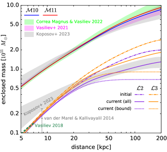
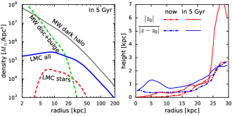
We consider two variants of models for each galaxy, with the halo parameters listed in Table 1. The Milky Way’s mass profile, shown in Figure 1, matches contemporary observational constraints (see e.g. Wang et al. 2020 for a compilation of recent estimates), with a virial mass being either for the lighter model 10 or for the heavier model 11. The initial mass of the LMC model is higher than the current estimates (see Figure 1 in V23 for a summary), but as it is tidally stripped on the first pericentre passage, its mass drops down to the acceptable range.
| model | | ||||||
|---|---|---|---|---|---|---|---|
| LMC halo | 2 | 8.95 | 160.9 | 150 | 1.92 | 2.0 | |
| 3 | 11.7 | 220.6 | 169 | 2.76 | 3.0 | ||
| MW halo | 10 | 15.0 | 500 | 260 | 10.0 | 11.8 | |
| 11 | 16.5 | 500 | 268 | 11.0 | 12.9 | ||
| MW stars see equations 2 and 3 in the text | 0.62 |
2.2 Simulation details
The simulations are conducted using the fast-multipole code gyrfalcON (Dehnen, 2000), augmented with a custom plugin for on-the-fly tracing of the centres of both galaxies. We use up to particles in the final highest-resolution runs, but the early stages are run with a reduced number of particles (by factors of 4 or 20). We set the softening length to 0.5 kpc for halo components and 0.2 kpc for the Milky Way stars (the equivalent Plummer softening length is smaller), and use a block timestep scheme with the smallest and largest timesteps of 0.5 Myr and 8 Myr, respectively. Since the public version of the code is not parallelized, a single full-resolution simulation takes hours.
We adopt the LMC centre position , and PM mas yr-1 from Gaia Collaboration (2021), distance of 49.6 kpc from Pietrzyński et al. (2019), and heliocentric line-of-sight velocity of 262.5 km s-1 from van der Marel et al. (2002). Using a right-handed Galactocentric reference system with the Solar position at {, 0, 0.02} kpc and velocity {12.9, 245.6, 7.8} km s-1 (Astropy collaboration, 2022; Drimmel & Poggio, 2018), this translates into the LMC position {, , } kpc and velocity {, , } km s-1. Of course, these quantities have non-negligible uncertainties, which have a significant impact on the past orbit reconstruction (see Figure 2 in V23 and associated discussion), but to facilitate the comparison between different simulations, we aim at reproducing the adopted position and velocity as precisely as possible.
The first guess for the initial phase-space coordinates of the LMC may come from integrating its test-particle orbit back in time in the static Milky Way potential, but this is very inaccurate for the massive LMC. A better guess could be obtained by integrating the coupled equations of motion of both galaxies as if they were rigid (non-deforming) but moving points sourcing their respective potentials, adding a drag force responsible for the dynamical friction (Gómez et al., 2015; Jethwa et al., 2016; Erkal et al., 2019). This approach is adopted in many studies (e.g., Laporte et al., 2018b; Garavito-Camargo et al., 2019; Petersen & Peñarrubia, 2020), but since the galaxies in live -body simulations are distorted in the interaction, their orbits deviate from the adopted ones. Previous studies attempted to minimize the deviation by tuning the amplitude of dynamical friction, or by iteratively refining the initial conditions using a grid search in the velocity space and picking up the closest point (e.g., Donaldson et al., 2022; Lilleengen et al., 2023)111Instead of a grid search, Guglielmo et al. (2014) used a genetic algorithm to tune the initial conditions, however, their simulations were not fully self-consistent (the Milky Way was modelled as a static potential).. However, the present-day position and velocity of the LMC are typically still off by a few kpc and few tens of km s-1– an error too large for an accurate reconstruction of the orbit.
In the present study, we aim to radically improve the precision of matching the final phase-space coordinates by iteratively adjusting the initial conditions . In each iteration, we run a master simulation with a given and a suite of companion simulations with slightly different initial conditions, and determine their final phase-space coordinates. Then we measure the Jacobian of the mapping from to and use it to assign the next guess for (a new value not chosen from the current suite). The entire process is then repeated several times until the mismatch in drops to an acceptable level ( kpc and 1 km s-1). The details of this procedure and associated challenges are described in the Appendix.
The LMC potential represents all particles that originated from the LMC, but many of them are no longer bound to it. To determine the bound mass, we use the following procedure: starting with all LMC particles, we construct their total potential and compute the particle energies in the reference frame associated with the LMC (i.e., subtracting its centre velocity from particle velocities when computing the kinetic energy). Then particles with are discarded, and the potential is recomputed from the remaining particles, followed by another round of eliminating particles with and repeating the cycle until convergence. The concept of bound mass is ill-defined in the case of an eccentric orbit, because some particles classified as unbound near the pericentre may be subsequently recaptured, but the above procedure gives a reasonable qualitative approximation. The lower set of curves in Figure 1 illustrate the enclosed mass profiles for two models, 2 and 3, in three variants: initial snapshot, current distribution of all particles originally belonging to the LMC system, and only the currently bound ones. These curves largely coincide within 20 kpc from the LMC centre, but start to deviate further out, with the bound mass essentially reaching a limit around 50 kpc. A comparison with the gray-shaded region representing dynamical constraints on the enclosed mass from the Orphan–Chenab stream modelling (Koposov et al., 2023) demonstrates that the two sets of LMC models are on the opposite ends of this range, and likely bracket the actual profile.
2.3 Resimulating the orbits in the approximated potential
For subsequent analysis, we construct smooth potential approximations for each snapshot in the simulation (stored every 64 Myr), separately for particles belonging to the LMC and to the Milky Way halo. It is convenient to work in the reference frame associated with the Milky Way centre. Because this frame is non-inertial, the total potential contains a spatially uniform but time-dependent UniformAcceleration term, which is obtained from the second derivative of the Milky Way trajectory (it is essential to smooth the trajectory beforehand, as otherwise the second derivative is far too noisy, see section 3.1.2 in Sanders et al. 2020). The Galactic stellar disc is approximated by the initial potential at all times, the Galactic halo is represented by a sequence of Multipole potentials pinned to origin, and the LMC is represented by a sequence of Multipole potentials moving along the smooth trajectory extracted from the simulation. We also created alternative BasisSet potential expansions, which use the Hernquist & Ostriker (1992) basis set and are compatible with other dynamical modelling packages such as Gala (Price-Whelan, 2017), though these are less efficient to evaluate than the Multipole expansions.
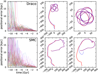
A natural question is whether such a time-dependent potential approximation provides a good description of the actual orbits of particles. Lowing et al. (2011) and Sanders et al. (2020) performed such accuracy analysis for the case of a single host halo from a cosmological simulation, in which there are no LMC-like massive satellites flying around, but numerous subhaloes create small-scale structures in the potential not captured by the low-order basis-set expansion. Nevertheless, it was found that most particle trajectories are well reproduced over the duration of the simulation. In our case, there are no small-scale substructures (apart from the dynamical friction-induced wake in the Milky Way halo), and the LMC is granted its own potential expansion, which moves along a smooth trajectory, so we may expect the fidelity of orbit reconstruction to be even better. Figure 2 shows a few examples of orbits from the actual simulation and their reconstructed counterparts, demonstrating that they stay fairly close (to within a few kpc) for the entire duration of simulation in most cases. Even if individual orbits may not be perfectly reconstructed, the ensemble of nearby orbits corresponding to a given satellite (Section 4.2) is very well reconstructed in the statistical sense. Re-running the entire simulation as an ensemble of non-interacting particles closely reproduces the current distribution and kinematics of Magellanic debris and the corresponding perturbations in the Milky Way halo.
After experimenting with different orders of expansion, we find that is more than sufficient, and we use 25 log-spaced nodes between 0.1 and 1000 kpc in the radial grids. Sanders et al. (2020) also compared the accuracy of orbit approximation in the case when the potential was taken from the nearest snapshot or linearly interpolated between snapshots, and found that the latter makes little difference but is twice more expensive (unless the expansion coefficients themselves are linearly interpolated before computing the potential, which is not available in Agama). However, we noticed that since the orbit integration in Agama uses a high-order method (dop853), the extra cost of a double potential evaluation is more than compensated by its increased smoothness, allowing the integrator to take larger timesteps. Even so, the computational cost (number of timesteps) scales with the requested accuracy as with for the nearest-timestamp potential and for the linearly interpolated potential, faster than the scaling expected for this integrator in an infinitely smooth potential. Nevertheless, a value of , while much coarser than the default used for analytic potentials, is sufficient for the relatively short duration of orbit integration (at most a few tens dynamical times).
3 Analysis
3.1 Orbital history of the LMC
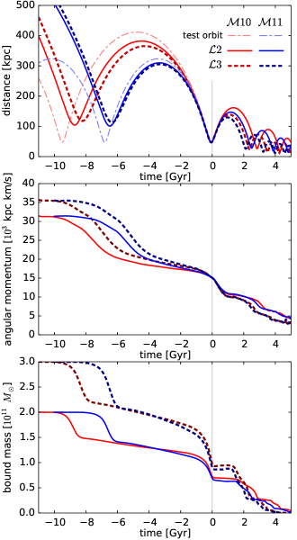
We first examine the past orbits of the LMC for different combinations of its mass and Galactic potential. Figure 3, top panel, shows the Galactocentric distance of the LMC in four simulations, together with test-particle orbits in the two Milky Way potentials 10, 11, shown by dot-dashed curves. It confirms the trend reported in V23: more massive LMC have smaller apocentre distances and shorter periods. This results from the interplay of two opposite effects. On the one hand, a more massive LMC experiences stronger dynamical friction, thus it must have started with a higher orbital energy to arrive to the same present-day phase-space point. On the other hand, though, a more massive LMC induces a larger reflex motion in the Milky Way, thus to achieve the same measured relative velocity, it needs to have a lower velocity in the centre-of-mass frame, meaning lower total energy and shorter period. Equivalently, the orbital period of the binary system depends on its total mass and is shorter for higher-mass LMC models. It turns out that the second factor outweighs the first one, though the difference in orbital period is rather minor between the two LMC models.
By contrast, the dependence of the orbital period on the Milky Way potential is quite dramatic, with difference between 10 and 11 (which differ by 10% in virial mass). As discussed in Section 3.2 of V23, this is due to the orbit being only marginally bound and the LMC currently located close to its pericentre, therefore its kinetic energy is almost equal in magnitude to its potential energy, and even a small variation in the latter leads to dramatic changes in the total energy. It is certainly possible to make the period comparable or longer than the Hubble time (i.e., put the LMC onto a first-approach trajectory), but the period could also be as short as 5–6 Gyr for a reasonable choice of Galactic potential. In these idealised simulations, we neglected the cosmological evolution of the Milky Way mass profile, which would have lengthened the orbital period (see Figure 11 in Kallivayalil et al. 2013), but also neglected other factors that could shorten it – the perturbation of the LMC velocity by the SMC or a favourable orientation of a non-spherical Milky Way potential (both discussed in V23). Overall, it is plausible that the previous passage of the LMC could have occurred between 5 and 10 Gyr ago at a distance just over 100 kpc, although the details may differ from our setup.
The middle and lower panels show the evolution of angular momentum and bound mass in these four simulations. Both quantities experience stepwise drops around each pericentre passage, but interestingly, the decrease of angular momentum occurs mostly after the pericentre, whereas the decrease of bound mass mostly precedes it. The bound mass during the past orbital period stays in the range (1.2–2), compatible with the current estimates (see Figure 1 in V23 for a compilation of literature values).
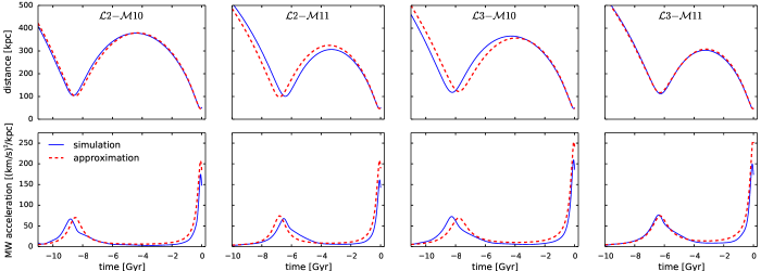
A popular approach for reconstructing the past orbit of the LMC, taking into account dynamical friction from the Galactic halo and reflex motion that the LMC induces on the Milky Way, is the solution of a coupled ODE system for two extended masses (Equation 1 in V23), using the gradient of gravitational potential of each galaxy at the current distance to compute the accelerations of both galaxies. It has been followed in many previous studies, e.g., Gómez et al. (2015), Jethwa et al. (2016), Erkal et al. (2019), Patel et al. (2020), Correa Magnus & Vasiliev (2022). As the Coulomb logarithm is generally treated as a tunable parameter, Hashimoto et al. (2003) found that a distance-dependent value provides a better match the results of actual -body simulations, with comparable to the scale radius of the satellite. The complication usually ignored by these studies is that the LMC mass also decreases with time, especially in the second-passage scenario. Figure 4 compares the actual orbits in our -body simulations (solid blue) with the solutions of the approximate ODE system (dashed red), in which the LMC mass has been set to half its initial value and set to . There are noticeable deviations in the reconstructed orbital periods (top row), and the LMC-induced acceleration of the Milky Way is overestimated by 20% at its peak (bottom row), because this prescription ignores the deformation of both galaxies. Although with two free parameters, we managed to match the grid of 4 simulations reasonably well, there is no guarantee that this recipe would be adequate for all reasonable choices of Milky Way and LMC mass profiles. It is clear that a more accurate approximation is highly desirable for a fast and reliable quantitative analysis, short of running the actual simulations.
3.2 Perturbations of the Milky Way halo
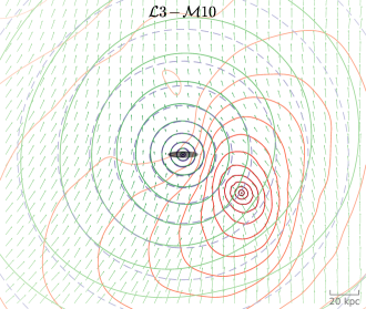
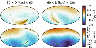
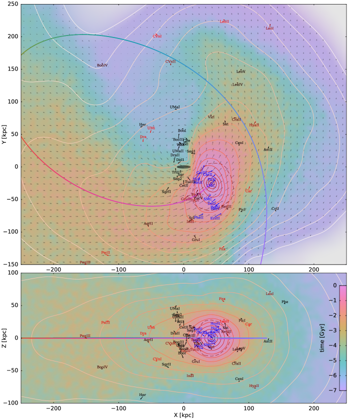
Middle row: heliocentric view of the density contrast in the Galactic halo. Left and right panels show the intermediate (30–60 kpc) and distant (60–120 kpc) regions. The past orbit of the LMC is shown by a solid green line when within this radial range, or by a dashed line otherwise, and its current location is indicated by a dot. Apart from the dynamical friction-induced overdensity along the orbit, there is a global dipole asymmetry primarily in the outer halo, corresponding to the downward shift of the Milky Way centre relative to its outer regions.
Bottom row: heliocentric view of the line-of-sight velocity of the Galactic halo in the same two radial ranges. The north–south dipole asymmetry is most prominent in the outer region.
As established in several recent studies (Garavito-Camargo et al., 2019, 2021a; Cunningham et al., 2020; Erkal et al., 2020, 2021; Petersen & Peñarrubia, 2020, 2021), a massive LMC induces significant perturbations in the Galactic halo at distances –30 kpc (see Section 4.2 in V23 for an extended discussion). A natural question is, therefore, whether the second-passage scenario produces different signatures from the first-passage scenario considered in the above papers.
Figure 5 shows the contours of Milky Way halo density projected onto the LMC orbital plane (top panel) and heliocentric sky maps of density and line-of-sight velocity perturbations (middle and bottom rows) in the 3–10 simulation. At a glance, these plots look very similar to the ones from the first-passage simulations (e.g., Figure 5 in V23). For a more detailed analysis, we constructed another simulation of a first passage, using the same Galactic model 10 and a lower-mass LMC model 2, started near the apocentre at time 4 Gyr ago. Of course, such a trajectory extrapolated further into the past would have had another pericentre passage, but we ignore this inconsistency for the sake of experiment. The density and kinematic perturbation maps in this scenario look so similar to Figure 5 that it is not even worth showing them separately. In other words, any possible signatures of the first passage either dissipate or are totally obscured by the most recent passage, which occurred at a twice smaller distance.
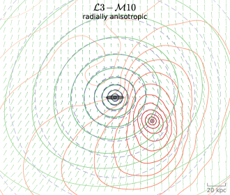
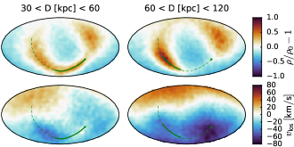
Models with the same LMC mass but different Milky Way potentials again look quite similar, and the variation of LMC mass only changes the amplitude of perturbations, but not their qualitative appearance. On the other hand, there are interesting differences between the models with isotropic Milky Way halo discussed so far, and a model with a radially anisotropic halo (, typical for the outer region of NFW haloes, e.g., Hansen & Moore 2006), which is shown in Figure 6. The velocity perturbations remain largely the same as in the previous figure, but the dynamical friction-induced overdensity along the past orbit of the LMC is much more prominent, and even more intriguingly, there is another overdensity along the future trajectory (upper left corner of the sky map). The large-scale dipole asymmetry is not significantly affected, but the local wake is strongly enhanced, in complete agreement with the study of Rozier et al. (2022), who used a very different method (linear response theory instead of conventional -body simulations). It is unclear which of the two cases better matches the current observations: a density asymmetry is much more difficult to measure reliably than a kinematic perturbation, and the only study which attempted this (Conroy et al., 2021) does not match either plot in detail (although they do note that the measured density contrast in the local wake is significantly higher than even in their simulation with the highest LMC mass of ). The previous orbital period of the LMC in the radially anisotropic halo is similar to its isotropic counterpart, but the initial angular momentum is higher and the distance of the first pericentre is correspondingly larger by ; in other words, radial anisotropy of the host galaxy enhances the radialization of satellite orbits, as already mentioned in Vasiliev et al. (2022).
It is also worth noting that the observationally determined direction of the dipole perturbation in line-of-sight velocities (Petersen & Peñarrubia, 2021) differs by more than 45∘ from the roughly north–south direction found in all simulations, including those in the present paper; the reasons for this discrepancy are not clear and may point to some deficiencies of current models, first or second passage alike.
3.3 Perturbations of the Galactic disc
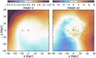
The LMC also imparts a noticeable perturbation on the Milky Way disc, likely contributing to the warp observed in its outer regions both in stars and gas. One should keep in mind that the very definition of the disc plane is not unambiguous. Here we use the particles within 10 kpc from the Galactic centre to construct a plane that minimizes the scatter of their coordinates relative to that plane. Although the initial models had aligned with the axis, by this best-fitting plane is already tilted by 1–1.5∘, which has an unintended consequence that the LMC coordinates in this rotated system are slightly different from the input values. Fortunately, the tilt direction is such that this offset roughly corresponds to a shift along the same trajectory by 3–4 Myr, so we ignore this minor deviation instead of trying to fit its present-day position in the rotated coordinate system.
Figure 7 shows the mean coordinate () of stars across the Galactic disc in the 3–11 simulation, which is qualitatively similar to other simulations. The noticeable warp in the top left corner is nearly opposite to the current location of the LMC ( kpc), and is caused by the same effect as the distortions in the Galactic halo, namely, that the inner part of the disc has shifted downward relative to the regions further away from the LMC. This displacement map qualitatively resembles Figure 6 in Laporte et al. (2018a), who conducted a similar set of simulations, though without matching the present-day LMC coordinates as precisely as in the present study. We stress that the perturbations rapidly evolve, e.g., the direction of the warp changes by over 0.1 Gyr, so for a quantitative analysis and comparison with observations, it is important to have a precisely fitted model. Here we do not attempt a detailed comparison, only noting that the warp in the model is similar to the one observed in stars (e.g., Figure 7 in Romero-Gómez et al. 2019, or Figure 2 in Lemasle et al. 2022), but somewhat smaller in amplitude. Laporte et al. (2018b) found that a combination of perturbations from the LMC and Sagittarius may create a stronger warp signature than a simple superposition, thus we do not expect our LMC-only models to match the data perfectly.
3.4 Future evolution
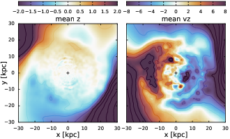
Given that our simulations produce an LMC model not only matching its observed present-day position and velocity, but also dynamically consistent with its prior evolution (i.e., with appropriate degree of tidal stripping), it makes sense to explore the future fate of the LMC and its effect on the Milky Way. We run the simulations for another 5 Gyr, and depending on the LMC mass, it completes another 3–4 orbits before being entirely disrupted (although the lowest-mass combination, 2–10, is not fully merged by the end of this interval). Figure 3 shows the future evolution of its mass and Galactocentric distance to the right of the vertical gray line.
Although the current magnitude of perturbations in the Galactic halo will not be exceeded in future pericentre passages due to the rapidly decreasing LMC mass, its effect on the Galactic disc will be more prominent as the pericentre radius drops to 25 kpc on the next passage, and then further to 10–15 kpc. Figure 8, top row, shows the maps of the disc warp similar to Figure 7, but at 5 Gyr in the future for the most massive combination 3–11, in which the LMC is fully disrupted by that time. The perturbations in the disc are much stronger than now, and it has become significantly hotter (lower right panel shows that the thickness has doubled across all radii) and tilted by relative to its initial orientation, but not destroyed.
Lower left panel of that figure shows the density profile of Magellanic debris, which has two characteristic break radii at 10 kpc (the radius of the last pericentre) and 40–50 kpc (the current pericentre radius). Although the initial LMC models did not have a separate stellar component, one could get a crude but sensible approximation by tracking 1% of most bound particles (the mass roughly matches the estimate of total stellar mass from van der Marel et al. 2002). The density of these particles is shown by red dashed line, and stays well below the density of Milky Way disc (dashed green) in the inner Galaxy, but may be comparable or even exceed the density of the pre-existing stellar halo at large distances. The total mass of present-day Milky Way stellar halo is estimated to be (Deason et al., 2019), so the LMC will quadruple it when fully disrupted. These findings agree well with the predictions of Cautun et al. (2019) based on Milky Way–LMC analogues in the EAGLE simulation, although in our experiments, it takes somewhat longer (4–5 Gyr) to fully destroy the LMC.
4 Galactic and Magellanic satellites
We now turn to the analysis of the population of dwarf galaxies surrounding the Milky Way (colloquially called Galactic satellites, although some of them are in fact satellites of the LMC).
4.1 Previous work
Lynden-Bell (1976) noticed that the dwarf galaxies Draco, Ursa Minor and Sculptor lie close to the plane of the Magellanic gas stream, itself discovered shortly before (Mathewson et al., 1974), and proposed that they are tidally stripped satellites of the postulated Great Magellanic Galaxy – the precursor of the LMC itself. Lynden-Bell (1982a) added Carina dSph to the list of galaxies possibly associated with the Great Magellanic Galaxy, while Lynden-Bell (1982b) introduced another dSph grouping – Fornax, Leo I, Leo II and Sculptor (FLS), but treated them separately from the Magellanic group, and Majewski (1994) added Sextans and Phoenix dSph to the FLS group. However, the planes of two groups differ by only , so Kroupa et al. (2005) proposed that they form a single group, later dubbed “Vast Polar Structure” by Pawlowski et al. (2012). Although a spatial alignment could happen by chance, it gradually became clear that most of these satellites also have similar directions of angular momentum (orbital poles), making this structure dynamically coherent (Metz et al., 2008; Pawlowski & Kroupa, 2013, 2020; Fritz et al., 2018).
D’Onghia & Lake (2008) proposed a Magellanic group consisting of 7 galaxies (two Clouds, Draco, Leo II, Sagittarius, Sextans and Ursa Minor), although they did not comment on why the orbital plane of Sagittarius is nearly orthogonal to that of the LMC. Metz et al. (2008) presented the now canonical list of clustered orbital poles of classical dwarfs: the Clouds, Carina, Draco, Fornax, Ursa Minor, and noted that if the Clouds were on their first passage and unrelated to the other four galaxies that have been orbiting the Milky Way for a while, it would be a rather unlikely coincidence for them to share the same orbital plane just by chance. Although the idea that a relatively thin and kinematically coherent disc of satellites could result from an accretion of a massive group of galaxies early in the Milky Way history is quite natural (e.g., Li & Helmi, 2008; Smith et al., 2016), somehow it did not get much traction, with Metz et al. (2009) arguing against it on the grounds that the observed plane of satellites in the Milky Way is too compact compared to the expectations from group accretion. Instead, Pawlowski et al. (2011) proposed a scenario in which the VPOS consists of “tidal dwarf galaxies” formed out of gas expelled during a tidal interaction between the Milky Way and another galaxy early in its evolution, somewhat reminiscent of the now abandoned Jeans–Jeffreys tidal theory of the Solar system formation (Jeffreys, 1952). They considered the possibility that the proto-LMC could be this intruder galaxy, though in their scenario the pericentre passage leading to the tidal stripping would have occurred at a much smaller distance ( kpc) than the most recent pericentre distance of the LMC (45–50 kpc).
| galaxy | L76 | D08 | M08 | N11 | J19 | P20 | E20 | S21 | B22 |
| Carina | ? | + | – | + | + | – | ? | ? | |
| Draco | + | + | + | + | – | ||||
| Fornax | + | ? | + | + | ? | ? | – | ||
| Leo I | – | – | |||||||
| Leo II | + | – | |||||||
| Sagittarius | + | – | + | – | |||||
| Sculptor | + | – | + | – | |||||
| Sextans | + | ? | – | ||||||
| Ursa Minor | + | + | + | + | – |
Until about 10 years ago, the census of Milky Way satellites was limited to relatively bright objects, whose association with the Magellanic system is difficult to establish with confidence (apart from the aforementioned similarity of orbital pole directions). Table 2 summarizes the proposed claims of Magellanic origin for classical dwarfs. However, since then many new ultrafaint galaxies were discovered in deep photometric surveys such as DES, and quite a few of them are very likely to be LMC satellites (see Table 1 in V23 for a compilation of results).
Numerous studies that considered the association of dSph and ultrafaint galaxies with the LMC system can be broadly divided into several categories:
-
1.
One may take the present-day positions and velocities of these objects as well as those of the LMC itself, then reconstruct the past orbit of the LMC in the assumed Galactic potential (ideally, not as a test particle moving in a fixed potential, but taking into account the reflex motion it induces on the Milky Way), and then follow the orbits of dwarf galaxies in the combined potential of the Milky Way and the LMC. An object can be declared an LMC satellite if it is currently bound to it, or a former satellite if it was bound at some point in the past (i.e., its relative velocity w.r.t. the LMC was below the escape velocity of the latter). Examples of this approach include Erkal & Belokurov (2020), Patel et al. (2020), Battaglia et al. (2022), Correa Magnus & Vasiliev (2022), Pace et al. (2022). The limitation of this approach is that it needs high-accuracy 6d phase-space coordinates of all objects for a reliable reconstruction of past orbits, which are rarely available, and even then the reconstruction becomes increasingly less reliable further into the past (e.g., D’Souza & Bell, 2022). This creates a bias against the association with the LMC system, since it is much more likely that the measurement errors will scatter an orbit away from the LMC than closer to it.
-
2.
To combat the latter problem, one may instead perform forward orbit modelling, namely, consider a large sample of particles initially bound to the LMC system, evolve their orbits forward up to the present time, and then identify which of the observed satellites are close to any of these LMC-associated particles within uncertainties. This alone is not enough to establish the likelihood of association – one needs to compare it with the alternative hypothesis that an object comes from the Milky Way system (or was accreted onto it independently from the LMC). This could be achieved by sampling an equally large number of particles from the Milky Way halo and counting the fraction of particles in the spatial and kinematic neighbourhood of each galaxy coming from the two alternative sources. The first part of this approach was followed in Nichols et al. (2011), Yozin & Bekki (2015), Jethwa et al. (2016), but these studies only examined whether a given dSph lies in the region occupied by the LMC debris (not even comparing the velocities due to a lack of measurements) without considering the alternative (non-LMC) origin.
-
3.
One can take this idea further and perform a full -body simulation of the two interacting galaxies, comparing the positions and velocities of observed dSph with the spatial and kinematic distribution of particles originating in both galaxies. Several groups have conducted simulations of this kind (Garavito-Camargo et al., 2019; Petersen & Peñarrubia, 2020; Vasiliev et al., 2021; Pawlowski et al., 2022; Makarov et al., 2023), but none so far have used them to assess the satellite population of the Magellanic system, although Vasiliev et al. (2021) employed this approach to determine the association of globular clusters with the Sagittarius galaxy (which was also simulated as a live -body system in that study). The challenge is to match the current position and velocity of the LMC with sufficient precision for this analysis to be meaningful, and only the latter study took great effort to meet it.
-
4.
Finally, one can resort to the analysis of cosmological simulations, either in large volume with thousands of Milky Way analogues, such as Millenium-II (Boylan-Kolchin et al., 2011), or more tailored Local Group-scale simulations, such as Aquarius (Sales et al., 2011, 2017; Kallivayalil et al., 2018), ELVIS (Deason et al., 2015), FIRE (Jahn et al., 2019), Auriga (Pardy et al., 2020) or Apostle (Santos-Santos et al., 2021). In this case the main challenge is to find suitable analogues of the Milky Way–LMC system, abandoning any hope for a detailed match, but only qualitatively reproducing its main properties. Earlier studies, such as Sales et al. (2011), did not find conclusive evidence of Magellanic association for any of the then-known dSph galaxies (except the SMC, of course), but with the more recent discoveries of numerous ultrafaint dwarfs in the vicinity of the LMC, several of them were proposed to be its satellites based on the similarity of their location (and sometimes velocity) to particles from LMC analogues in the simulations. Jahn et al. (2019) and Pardy et al. (2020) also proposed Carina and Fornax as possible former satellites of the LMC, based on their updated PM from Gaia DR2, but Santos-Santos et al. (2021) found this possibility rather tenuous.
In this study, we take the third approach, analyzing the possible origin of each dSph by comparing its phase-space coordinates with particles in the simulation. We also use elements of the second approach, rewinding dSph orbits in the pre-recorded potential of the simulation approximated by smooth potential expansions and comparing the probability of arriving with the Magellanic system against originating in the Milky Way. We take the coordinates, distances and line-of-sight velocities from the catalogue of McConnachie (2012, updated in 2021)222https://www.cadc-ccda.hia-iha.nrc-cnrc.gc.ca/en/community/nearby/, and Gaia eDR3 PM from Battaglia et al. (2022); the SMC PM is taken from Gaia Collaboration (2021).
4.2 Satellites in our simulations
Let be the 6d vector of observable phase-space coordinates of a given object (longitude , latitude , distance , two PM components , , and line-of-sight velocity )333Here longitude and latitude are not in the Galactic coordinate system, but rather in a system rotated such that the target object is at origin, minimizing distortions of the PM field that could appear for objects near celestial poles., and be the covariance matrix of measurement uncertainties (in case of uncorrelated errors, it is diagonal with squared standard deviations in each coordinate ). Although the position is measured essentially perfectly, we need to introduce an artificial uncertainty in celestial coordinates in order to have a sufficient number of particles to match, setting . We also put a lower limit on the uncertainty in distance (), line-of-sight velocity (km s-1) and PM (mas yr-1), both to increase the chance of matching and to account for various systematic deviations between the model and the real Milky Way. The -body snapshot is then converted into the same coordinates , . To determine the probability of the object to belong to either the LMC or the Milky Way, we use three different approaches.
In the first method (particle matching), we compute the uncertainty-weighted Mahalanobis distance between the object and each -body particle: . The matching likelihood for -th particle is , where is the mass of this particle, and the overall coefficient of proportionality determined from the condition that . Then the probability of association with the LMC is simply the sum of over particles that originally belonged to the LMC. One can obtain a representative sample of past orbits by selecting particles in proportion to their likelihood of matching and retrieving their trajectories from the original simulation. This method is the most direct, but may suffer from low-number statistics even in the highest-resolution snapshots, if the number of particles with sufficiently high matching probabilities is too small. In these cases, we artificially increase the uncertainties on kinematic measurements ( and ) until the highest matching probability is below 0.1 (i.e., there are at least 10 different matches).
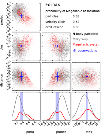
In the second method, we limit the matching to the spatial dimensions (, , ), obtaining a much larger sample (typically a few thousand particles) that are close to the target object in space. We select particles with sufficiently small Mahalanobis distance from the target object in the three spatial dimensions (), and their contribution to the distribution of each population (LMC or Milky Way) is weighted by the probability of spatial matching , so that the total mass of particles in each population is . Then we construct two Gaussian mixture models, one for the Milky Way particles and the other for the particles originating in the Magellanic system. Each population is described by Gaussian components in the entire 6d space of observables, with amplitudes , means and covariance matrices , where the sum of amplitudes for each population is . Since particle weights are pre-multiplied by the probability of spatial matching, the distributions in these three dimensions are nearly Gaussian by construction; nevertheless, this procedure still allows one to recover correlations between spatial and kinematic dimensions, which are sometimes important for the LMC debris. The probability distribution of the given population (LMC or Milky Way) in the entire 6d space is given by
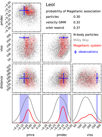
To account for observational uncertainties, this probability distribution should be convolved with the Gaussian error distribution described by the error covariance matrix , which for a Gaussian mixture model amounts to adding to in the above equation. Here the uncertainties in the spatial dimensions should be to a very large number (formally, infinity), since we have already preselected particles according to their spatial matching probability, so no further convolution is needed (this effectively amounts to marginalizing over these dimensions). Finally, the probability of the object to belong to -th population is simply . The advantage of this method over the first one is that the smooth probability distributions are constructed from a much larger number of particles, but evaluated only in a possibly narrow range of kinematic coordinates, thus effectively interpolating them in a region where the actual number of matching particles could be rather small. The method is illustrated in Figure 9 for two galaxies, Fornax and Leo I.
The third method does not use the -body snapshot directly, but instead relies on orbit integrations in the evolving gravitational potential described by a series of multipole expansions, as detailed in Section 2.3. Namely, we sample points from the uncertainty distribution described by the mean coordinates and the error covariance matrix . Then we integrate the orbits back in time from these initial conditions to the starting point of the simulation (10–11 Gyr ago), when the LMC was still approaching the Milky Way from a distance of a few hundred kpc. At this point, one may be tempted to simply count the fraction of orbits that end up being bound to the LMC at that time, as was done in most previous studies, but this will not give a correct answer, because not all points in our initial conditions are equally probable a posteriori. To illustrate the fallacy, consider the case of very large PM uncertainties (e.g., Pisces II) and/or missing line-of-sight velocity (e.g., Delve 2). Most of the rewound orbits would miss the LMC by a large margin, but they would also be unbound from the Milky Way or have apocentres well beyond the virial radius, making these orbits unlikely to appear in our simulation. Even if the uncertainties are small, the unweighted fraction of LMC-bound orbits tends to be underestimated, sometimes quite severely. Instead, one needs to weigh each orbit with the probability of finding it among the initial conditions of our simulations, which consist of two equilibrium galaxy models. So we again use a mixture model approach, but instead of Gaussians in the present-day observable coordinates, we use the distribution functions of initial models normalized such that the integral of over the entire 6d phase space is the total mass of each galaxy (or just its dark halo, in the case of Milky Way). Of course, in this evaluation we need to consider relative positions and velocities of particles with respect to each galaxy’s centre , and set to zero if the relative velocity exceeds the escape velocity. The un-normalized likelihood of association with either population is , and the normalized probability of association is again . This approach is similar to the one used in Correa Magnus & Vasiliev (2022), except that here we have a mixture of two populations bound to each galaxy, instead of just the Milky Way halo plus the “unmixed” population as in that paper. Since relatively few objects (mostly distant dSph) were found to be unmixed, and none of them are likely to be associated with the LMC, we ignore this component in the present study.
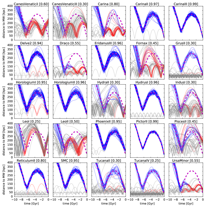
Reassuringly, all three methods agree remarkably well (to within 10% difference in probability) for the vast majority of objects, so in the summary Table 3 we provide a single value (average between three methods) for each galaxy in each of the four simulations, skipping objects with less than 10% probability of Magellanic association. These objects can be grouped into two classes. Eleven of them are likely to be Magellanic satellites at present time: Carina II, Carina III, Delve 2, Eridanus III, Horologium I, Horologium II, Hydrus I, Phoenix II, Pictor II, Reticulum II and SMC. The probabilities exceed 90% (except Reticulum II, which is only 80%), despite three of these galaxies lacking line-of-sight velocity measurements (Delve 2, Eridanus III and Pictor II). This classification broadly agrees with most recent studies (e.g., Fritz et al. 2019, Erkal & Belokurov 2020, Patel et al. 2020, Battaglia et al. 2022, Correa Magnus & Vasiliev 2022, Pace et al. 2022, see Table 1 in V23 for a compilation). Figure 10 shows that these galaxies, shown by blue colour, are indeed located within the region occupied by particles still bound to the LMC (brown dashed contour) and move in the same direction.
Perhaps more interestingly, many of the remaining galaxies in Table 3, shown by shades of red in the above figure, have a significant probability of association with the LMC, even though they are not currently bound to it. In particular, four of the classical dSph – Carina, Draco, Fornax and Ursa Minor – have a roughly equal chance to either be accreted with the Magellanic system or originate from elsewhere (in case of Carina, the chances are even higher, ). A distant galaxy Leo II has a probability of Magellanic association between 0.3 and 0.5, and even the peculiar Leo I, the least bound object in this sample, has a non-negligible chance of association in the 3 series of models444We remind that regardless of whether Leo I is associated with the LMC or not, its current velocity relative to the Milky Way centre has been increased by a few tens km s-1 due to the reflex motion of the Milky Way caused by the recent LMC flyby (Erkal et al., 2020; Correa Magnus & Vasiliev, 2022).. Even some galaxies with missing velocity components might be associated with the LMC under certain conditions; Table 4 lists the predicted PM and line-of-sight velocity values assuming such an association. Summing up the probabilities of galaxies in this group, we may conjecture that the original Magellanic system might have brought in some 4–6 galaxies that became Milky Way satellites, half of them in the mass range of classical dSph. They would populate the unusual 12 magnitudes luminosity gap between the SMC and other ultrafaint LMC satellites highlighted by Dooley et al. (2017) and Pardy et al. (2020), and indeed the latter study suggested that Carina and/or Fornax might fill this gap.
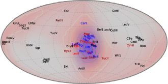
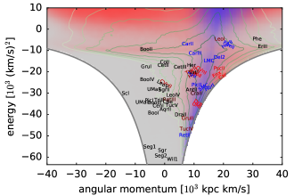
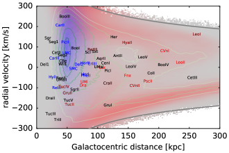
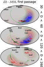
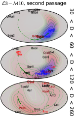
Figure 11 shows the distribution of Magellanic and Milky Way particles in different kinematic spaces: orbital pole orientation (top panel), energy–angular momentum (middle panel) and Galactocentric radius–velocity (bottom panel), and the locations of observed galaxies in these spaces. Particles still bound to the LMC and galaxies from the first group are well localized in each of these spaces, but possible former LMC satellites are considerably scattered and mixed with native Milky Way satellites in any particular projection, justifying the need for a full 6d analysis as in the present study. The distribution of former satellites in orbital phase is quite asymmetric, with all but one object (Pisces II) populating the leading arm of the tidal debris stream (the trailing arm is visible as the red band in the lower part of the bottom panel). A similar situation occurs with the globular clusters stripped from the Sagittarius galaxy, and the reason for this asymmetry is currently unknown. As the census of Milky Way satellites is very likely still incomplete (Koposov et al., 2009; Jethwa et al., 2016), one may use these “finding charts” to assess the possibility of Magellanic association of any object discovered in the future, though only if we have kinematic information. Figure 12 instead shows just the observable sky-plane distribution of LMC debris in different distance bins, both for first-passage (left) and second-passage (right) simulations. Unfortunately, the difference between these scenarios is not very dramatic, and mostly seen in the outermost distance bin and in the Northern hemisphere, which cannot be reached by debris from a single passage.
Figure 13 shows possible past orbits of selected galaxies in one of the simulations (3–11), illustrating that the galaxies from the second group have been stripped after the first pericentre passage, and their subsequent orbits do not resemble that of the LMC, but still stay roughly in the same orbital plane. This kinematic peculiarity, of course, has been known for a long time, as discussed in Section 4.1, but here we provide an explicit demonstration that such an arrangement is a natural outcome of the tidal stripping of a massive Magellanic system.
| Name | 210 | 211 | 310 | 311 | ||
| Canes Venatici I | 210 | 0.1 | 0.3 | 0.3 | 0.6 | |
| Canes Venatici II | 160 | 0.3 | 0.35 | 0.35 | 0.3 | |
| Carina | 106 | 0.55 | 0.65 | 0.7 | 0.8 | |
| Carina II | 37 | 0.97 | 0.95 | 0.98 | 0.97 | |
| Carina III | 28 | 0.99 | 0.99 | 0.99 | 0.99 | |
| Crater II | 117 | 0.2 | 0.1 | 0.1 | 0.1 | |
| Delve 2 | 71 | 0.93 | 0.91 | 0.95 | 0.94 | |
| Draco | 76 | 0.4 | 0.45 | 0.55 | 0.55 | |
| Eridanus III | 91 | 0.95 | 0.95 | 0.97 | 0.96 | |
| Fornax | | 147 | 0.4 | 0.4 | 0.5 | 0.45 |
| Grus II | 55 | 0.25 | 0.25 | 0.3 | 0.3 | |
| Horologium I | 79 | 0.92 | 0.90 | 0.94 | 0.95 | |
| Horologium II | 78 | 0.95 | 0.94 | 0.97 | 0.96 | |
| Hydra II | 151 | 0.2 | 0.3 | 0.3 | 0.3 | |
| Hydrus I | 28 | 0.95 | 0.95 | 0.96 | 0.96 | |
| Indus I | 105 | 0.2 | 0.2 | 0.3 | 0.3 | |
| Leo I | | 258 | 0.15 | 0.1 | 0.3 | 0.25 |
| Leo II | 233 | 0.3 | 0.4 | 0.4 | 0.5 | |
| Phoenix II | 83 | 0.95 | 0.93 | 0.96 | 0.95 | |
| Pictor II | 46 | 0.99 | 0.99 | 0.99 | 0.99 | |
| Pisces II | 183 | 0.2 | 0.3 | 0.35 | 0.45 | |
| Reticulum II | 31 | 0.8 | 0.75 | 0.85 | 0.8 | |
| Reticulum III | 92 | 0.1 | 0.1 | 0.25 | 0.15 | |
| SMC | | 63 | 0.92 | 0.92 | 0.95 | 0.95 |
| Tucana II | 58 | 0.3 | 0.2 | 0.35 | 0.3 | |
| Tucana IV | 47 | 0.2 | 0.2 | 0.3 | 0.25 | |
| Ursa Minor | 76 | 0.45 | 0.45 | 0.45 | 0.55 | |
| Virgo I | 91 | 0.1 | 0.1 | 0.1 | 0.1 |
| Name | |||
|---|---|---|---|
| Delve 2 | |||
| Eridanus III | |||
| Indus I | |||
| Pegasus III | |||
| Pictor I | |||
| Pictor II | |||
| Pisces II | |||
| Virgo I |
Pawlowski et al. (2011) proposed that the disc of satellites consists of tidal dwarf galaxies formed out of gas that was tidally stripped from the progenitor galaxy (possibly the proto-Magellanic system) during its pericentre passage. In our view, this scenario is conceptually similar to the one considered in the present paper, except that we assume that these galaxies were already formed before the first pericentre passage of the Magellanic system, but the stripping mechanism is the same, so we remain agnostic as to whether these galaxies are expected to be “primordial” (formed in the standard cosmological paradigm) or “second generation” (formed out of tidally stripped gas without necessarily be embedded in dark matter haloes). Full hydrodynamical simulations may be needed to resolve this question.
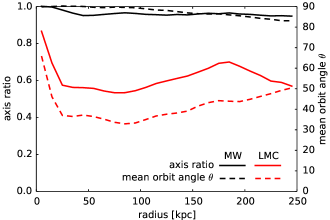
Although thin satellite planes appear to be quite rare around generic Milky Way-mass host galaxies in cosmological simulations (see Section 2.2.3 in Pawlowski 2021 for a review of relevant literature), Samuel et al. (2021) found that the fraction of satellite planes significantly increases if one selects host galaxies that have an LMC analogue near its pericentre. Garavito-Camargo et al. (2021b) suggested that the dynamical perturbation from the LMC may enhance the apparent clustering of orbital poles due to direct deflection of orbits by the LMC flyby and the global displacement of the Milky Way-centred reference frame relative to the outer halo. On the other hand, Pawlowski et al. (2022) and Correa Magnus & Vasiliev (2022) found that this effect alone is insufficient to account for the observed VPOS thinness. After excluding the current LMC satellites and rewinding the orbits of remaining objects in the combined Milky Way–LMC potential back in time to undo the LMC perturbation, the clustering of orbital poles was not significantly affected. To complement this analysis, Figure 14 shows the asymmetries in the spatial distribution (axis ratio of the moment of inertia tensor) and in kinematics (mean angle between the angular momentum of particles relative to that of the LMC) of particles in our simulations, separately for the Milky Way (black) and Magellanic particles (red). It is clear that the perturbations in the native Milky Way halo population are minimal – the orbital poles of particles stay very close to isotropic () within 100 kpc and only show a slight enhancement in the direction of the LMC orbital pole further out, confirming the results of Pawlowski et al. (2022). By contrast, particles belonging to the Magellanic debris have a prominent concentration of their orbital poles () and are more flattened (axis ratio 1:2), although the observed satellite plane is still thinner.
However, these idealised simulations may not be representative of the evolution of Galactic satellite distribution in a realistic cosmological context. Following upon the work of Samuel et al. (2021), Garavito-Camargo et al. (2023) considered Milky Way–LMC analogues in the Latte cosmological simulations, and found that the enhancement of orbital pole concentration is more prominent than in isolated simulations of Milky Way–LMC encounter, although the displacement of the inner Galaxy w.r.t. the outer halo remains the driving mechanism. However, this enhancement persist only for a short time around the pericentre passage of the LMC analogue: using the IllustrisTNG cosmological simulations, Kanehisa et al. (2023) found that such encounters do not produce long-lived satellite planes. This result is at odds with our conclusion that the objects stripped on the first passage remain close to the LMC orbital plane; the discrepancy might be caused by the idealised (non-cosmological) nature of our simulations.
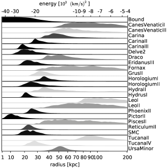
Figure 15 shows the possible origins of galaxies that were part of the Magellanic system, expressed as the percentile of their initial binding energy among all LMC particles. Naturally, the eleven galaxies from the first group (current LMC satellites) must have started rather deep inside its potential in order to avoid being stripped on the first passage, but not too tightly bound (with the exception of Pictor II) to avoid tidal disruption by the LMC itself. Galaxies from the second group have generally broader distributions of possible initial binding energies, but still avoiding least bound orbits, which may explain their stronger spatial and dynamical coherence compared to the entire distribution of Magellanic debris shown on the previous figure.
We also examined the probability of Magellanic association of dSphs for the simulation of a single passage (210 run for 4 Gyr). In this case, all eleven galaxies from the first group are still highly likely to be current LMC satellites, but among the second group, only Carina retains a significant (40–50%) probability of association, Grus II, Hydra II, Pisces II and Tucana II stay at the level 20–40%, and remaining galaxies are not compatible with the distribution of Magellanic debris. Thus the ability to explain the existence of the satellite plane is an important argument in favour of the second-approach model in the standard cosmological paradigm. The alternative scenario advocated by Pawlowski & Kroupa (2013) and subsequent studies involves modified Newtonian gravity theories (e.g., MOND, Milgrom 1983), in which case it is the early encounter with M31 rather than LMC that could give rise to the dynamically coherent second-generation tidal dwarf galaxy population (Bílek et al., 2018; Banik et al., 2022).
5 Discussion
Although most studies in the last decade concentrated on the first passage (or recent infall) scenario for the Magellanic clouds, in this study we demonstrate that the alternative scenario in which they had another pericentre passage 5–10 Gyr ago does not violate any observational constraints:
-
•
The updated measurement of the LMC PM with HST (Kallivayalil et al., 2013) and Gaia (Gaia Collaboration, 2021) led to a downward revision of the LMC tangential velocity by a few tens km s-1 compared to the earlier HST measurement by Kallivayalil et al. (2006). Whereas the latter would make the LMC orbit unbound unless the Milky Way mass is well above , the updated PM makes it comfortably bound even if is around , as preferred by most recent estimates (Section 3.1).
-
•
A high initial LMC mass () shortens the inferred orbital period, but increases the distance of the previous pericentre passage to kpc. At this distance, the tidal radius of the LMC is large enough that it has no problem of retaining all satellites that are currently still orbiting it, including the SMC (Section 4.2).
-
•
The perturbations of the Milky Way halo induced by the LMC during its current flyby look nearly the same in the first- and second-passage scenarios, and qualitatively agree with the observed signatures, though some deviations remain unexplained (Section 3.2).
The latter circumstance is rather unfortunate, as one would like to have a definite prediction or observed signature that would distinguish the two scenarios. Although we do not have a smoking-gun evidence in favour of the second-passage scenario, a strong argument in its support is the natural emergence of the spatially and kinematically coherent plane of satellites as a product of tidal stripping during the previous pericentre passage. We stress that our analysis does not aim to quantify how common or unusual is this structure – it may well be that the Milky Way–LMC system is rather special (e.g., Busha et al., 2011). It also does not address the likelihood of a particular configuration of objects within the orbital plane of the LMC: for instance, the results would not change if all galaxies were concentrated in the same spatial region rather than being uniformly spread in angles. It merely evaluates the conditional probability of a given object to come from the Magellanic system, given its current position and velocity and a plausible history of interaction between the Milky Way and the LMC. We find that in the second-passage scenario, most galaxies with orbital poles similar to that of the LMC indeed have a large probability of past association, whereas if the LMC is on its first approach, only Carina dSph could be possibly coming alongside it.
Our simulations and analysis have a number of limitations and simplifying assumptions, some of which can be addressed in the follow-up work:
-
•
We only considered a small number of models, focusing on the dependence of the orbital period on the Milky Way and LMC masses. It would be interesting to vary the shape of the Galactic potential, as it also has a significant effect on the orbital period (Figure 4 in V23).
-
•
We modelled the LMC as a single spherical halo, without explicitly introducing a stellar component. The actual LMC has a (thick) stellar disc with a bar, whose formation might have been triggered by the previous pericentre passage (e.g., Lokas et al., 2014), although it is more likely to result from its interaction with the SMC.
-
•
Speaking of the latter, the neglect of the gravitational pull from LMC’s most massive satellite does have a substantial effect on its inferred orbit. Although some studies (e.g., Jethwa et al. 2016, Patel et al. 2020) considered the three-body interaction of Milky Way, LMC and SMC using simple orbit integrations, it has not yet been studied in full -body simulations. The problem of matching the current position and velocity of both Magellanic Clouds could be too challenging, so a simulation of the live SMC in the pre-recorded time-dependent potential of the Milky Way and LMC (similar to the simulations of Sagittarius dSph conducted in Vasiliev et al. 2021) might be an intermediate step. Even if the SMC is much less massive than the LMC, it still shifts the centre of mass of both Clouds and reduces their Galactocentric orbital period (Figure 3 in V23).
-
•
Our simulations were pure -body, but the Clouds contain a substantial amount of gas. In the currently dominant first-passage scenario, the Magellanic gas stream results from the interaction of the two Clouds (Besla et al., 2010). It would be very interesting to examine the formation mechanisms of the Magellanic stream in the second-passage scenario.
-
•
It is also rather inconvenient that one has to run an entire -body simulation to reliably reconstruct the past trajectory of the LMC, as the approximate orbit integration method, while very fast, is not accurate enough (Figure 4). A yet-to-be-developed hybrid method for approximating the orbital and mass loss evolution that sits between these two extremes would be very valuable for extensive exploration of parameter space (e.g., of the Milky Way potential).
-
•
The analysis of observational constraints on the star formation histories of the Magellanic Clouds and other dwarf galaxies may help to constrain their past orbital histories (e.g., Hasselquist et al., 2021; Mazzi et al., 2021; Massana et al., 2022), supporting or disfavouring the proposed scenario.
-
•
The reconstruction of past trajectories of satellites assumed them to be point masses, i.e., ignored the tidal stripping. Some of the LMC satellites might not have survived on their inferred orbits with fairly small pericentre distances and short periods, though the range of possible past orbits is usually large enough to accommodate less stressful ones. Still, the evolution of LMC satellites in the tidal field is worth exploring in more detail.
To facilitate future studies of these and other related questions, we provide the simulation snapshots, time-dependent potentials, scripts for their analysis and for tailoring the orbital initial conditions, in a public Zenodo repository. For instance, one could use them for quickly evaluating the probability of Magellanic association for any newly discovered satellites (with or without kinematic information).
It is clear that the presence of the Magellanic Clouds in such a special configuration (near their pericentre) is a rather peculiar feature of Milky Way dynamics. As demonstrated in this study, even the basic question about when they have been accreted does not have a definite answer at the current level of knowledge, though we provided arguments in favour of the second-passage scenario. That the answer is highly sensitive to various parameters makes them an excellent tool for exploring the structure and past history of our Galaxy, and the Clouds are very welcome even for that reason alone, not to mention their sheer beauty.
Acknowledgements: I thank many of my colleagues at Edinburgh and Cambridge for stimulating discussions and comments, in particular, Mike Petersen, whose request to share the script for fitting the orbital initial conditions prompted me to significantly improve it, in turn enabling a reliable analysis of second-passage orbits. I also thank the referee for valuable comments that helped to improve the presentation.
Data availability: The simulation data and associated scripts are provided at https://zenodo.org/record/8015660.
References
- Astropy collaboration (2022) Astropy collaboration (Price-Whelan et al.), 2022, ApJ, 935, 167; ascl:1304.002
- Banik et al. (2022) Banik I., Thies I., Truelove R., Candlish G., Famaey B., Pawlowski M., Ibata R., Kroupa P., 2022, MNRAS, 513, 129
- Battaglia et al. (2022) Battaglia G., Taibi S., Thomas G., Fritz T., 2022, A&A, 657, 54
- Besla et al. (2007) Besla G., Kallivayalil N., Hernquist L., Robertson B., Cox T., van der Marel R., Alcock C., 2007, ApJ, 668, 949
- Besla et al. (2010) Besla G., Kallivayalil N., Hernquist L., van der Marel R., Cox T., Kereš D., 2010, ApJ, 721, L97
- Bílek et al. (2018) Bílek M., Thies I., Kroupa P., Famaey B., 2018, A&A, 614, 59
- Boylan-Kolchin et al. (2011) Boylan-Kolchin M., Besla G., Hernquist L., 2011, MNRAS, 414, 1560
- Busha et al. (2011) Busha M., Wechsler R., Behroozi P., Gerke B., Klypin A., Primack J., 2011, ApJ, 743, 117
- Cautun et al. (2019) Cautun M., Deason A., Frenk C., McAlpine S., 2019, MNRAS, 483, 2185
- Conroy et al. (2021) Conroy C., Naidu R., Garavito-Camargo N., Besla G., Zaritsky D., Bonaca A., Johnson B., 2021, Nature, 592, 534
- Correa Magnus & Vasiliev (2022) Correa Magnus L., Vasiliev E., 2022, MNRAS, 511, 2610
- Cunningham et al. (2020) Cunningham E., Garavito-Camargo N., Deason A., et al., 2020, ApJ, 898, 4
- Deason et al. (2015) Deason A., Wetzel A., Garrison-Kimmel S., Belokurov V., 2015, MNRAS, 453, 3568
- Deason et al. (2019) Deason A., Belokurov V., Sanders J., 2019, MNRAS, 490, 3426
- Dehnen (2000) Dehnen W., 2000, ApJ, 536, L9; ascl:1402.031
- D’Onghia & Lake (2008) D’Onghia E., Lake G., 2008, ApJ, 686, L61
- Donaldson et al. (2022) Donaldson K., Petersen M., Peñarrubia J., 2022, MNRAS, 513, 46
- Dooley et al. (2017) Dooley G., Peter A., Carlin J., Frebel A., Bechtol K., Willman B., 2017, MNRAS, 472, 1060
- Drimmel & Poggio (2018) Drimmel R., Poggio E., 2018, RNAAS, 2, 210
- D’Souza & Bell (2022) D’Souza R., Bell E., 2022, MNRAS, 512, 739
- Erkal et al. (2019) Erkal D., Belokurov V., Laporte C., et al., 2019, MNRAS, 487, 2685
- Erkal & Belokurov (2020) Erkal D., Belokurov V., 2020, MNRAS, 495, 2554
- Erkal et al. (2020) Erkal D., Belokurov V., Parkin D., 2020, MNRAS, 498, 5574
- Erkal et al. (2021) Erkal D., Deason A., Belokurov V., et al., 2021, MNRAS, 506, 2677
- Fritz et al. (2018) Fritz T., Battaglia G., Pawlowski M., et al., 2018, A&A, 619, 103
- Fritz et al. (2019) Fritz T., Carrera R., Battaglia G., Taibi S., 2019, A&A, 623, 129
- Gaia Collaboration (2018) Gaia Collaboration (Helmi et al.), 2018, A&A, 616, 12
- Gaia Collaboration (2021) Gaia Collaboration (Luri et al.), 2021, A&A, 649, 7
- Garavito-Camargo et al. (2019) Garavito-Camargo N., Besla G., Laporte C., Johnston K., Gómez F., Watkins L., 2019, ApJ, 884, 51
- Garavito-Camargo et al. (2021a) Garavito-Camargo N., Besla G., Laporte C., Price-Whelan A., Cunningham E., Johnston K., Weinberg M., Gómez F., 2021, ApJ, 919, 109
- Garavito-Camargo et al. (2021b) Garavito-Camargo N., Patel E., Besla G., Price-Whelan A., Gomez F., Laporte C., Johnston K., 2021, ApJ, 923, 140
- Garavito-Camargo et al. (2023) Garavito-Camargo N., et al., 2023, submitted
- Gómez et al. (2015) Gómez F., Besla G., Carpintero D., Villalobos Á., O’Shea B., Bell E., 2015, ApJ, 802, 128
- Guglielmo et al. (2014) Guglielmo M., Lewis G., Bland-Hawthorn J., 2014, MNRAS, 444, 1759
- Hansen & Moore (2006) Hansen S., Moore B., 2006, New Astron., 11, 333
- Hashimoto et al. (2003) Hashimoto Y., Funato Y., Makino J., 2003, ApJ, 582, 196
- Hasselquist et al. (2021) Hasselquist S., Hayes C., Lian J., et al., 2021, ApJ, 923, 172
- Hernquist & Ostriker (1992) Hernquist L., Ostriker J., 1992, ApJ, 386, 375
- Jahn et al. (2019) Jahn E., Sales L., Wetzel A., Boylan-Kolchin M., Chan T., El-Badry K., Lazar A., Bullock J., 2019, MNRAS, 489, 5348
- Jeffreys (1952) Jeffreys H., 1952, Proc.R.Soc.London, series A, 214, 281
- Jethwa et al. (2016) Jethwa P., Erkal D., Belokurov V., 2016, MNRAS, 461, 2212
- Kallivayalil et al. (2006) Kallivayalil N., van der Marel R., Alcock C., Axelrod T., Cook K., Drake A., Geha M., 2006, ApJ, 638, 772
- Kallivayalil et al. (2013) Kallivayalil N., van der Marel R., Besla G., Anderson J., Alcock C., 2013, ApJ, 764, 161
- Kallivayalil et al. (2018) Kallivayalil N., Sales L., Zivick P., et al., 2018, ApJ, 867, 19
- Kanehisa et al. (2023) Kanehisa K., Pawlowski M., Müller O., 2023, arXiv:2307.03218
- Koposov et al. (2009) Koposov S., Yoo J., Rix H.-W., Weinberg D., Macciò A., Miralda-Escudé J., 2009, ApJ, 696, 2179
- Koposov et al. (2023) Koposov S., Erkal D., Li T.S., et al., 2023, MNRAS, 521, 4936
- Kroupa et al. (2005) Kroupa P., Theis C., Boily C., 2005, A&A, 431, 517
- Laporte et al. (2018a) Laporte C., Gómez F., Besla G., Johnston K., Garavito-Camargo N., 2018a, MNRAS, 473, 1218
- Laporte et al. (2018b) Laporte C., Johnston K., Gómez F., Garavito-Camargo N., Besla G., 2018b, MNRAS, 481, 286
- Lemasle et al. (2022) Lemasle B., Lala H., Kovtyukh V., et al., 2022, A&A, 668, 40
- Li & Helmi (2008) Li Y.-S., Helmi A., 2008, MNRAS, 385, 1365
- Lilleengen et al. (2023) Lilleengen S., Petersen M., Erkal D., et al., 2023, MNRAS, 518, 774
- Lokas et al. (2014) Lokas E., Athanassoula E., Debattista V., Valluri M., del Pino A., Semczuk M., Gajda G., Kowalczyk K., 2014, MNRAS, 445, 1339
- Lowing et al. (2011) Lowing B., Jenkins A., Eke V., Frenk C., 2011, MNRAS, 416, 2697
- Lynden-Bell (1976) Lynden-Bell D., 1976, MNRAS, 174, 695
- Lynden-Bell (1982a) Lynden-Bell D., 1982a, The Observatory, 102, 7
- Lynden-Bell (1982b) Lynden-Bell D., 1982b, The Observatory, 102, 202
- Majewski (1994) Majewski S., 1994, ApJ, 431, L17
- Makarov et al. (2023) Makarov D., Khoperskov S., Makarov D., Makarova L., Libeskind N., Salomon J.-B., 2023, MNRAS, 521, 3540
- Massana et al. (2022) Massana P., Ruiz-Lara T., Noël N., et al., 2022, MNRAS, 513, L40
- Mathewson et al. (1974) Mathewson D., Cleary M., Murray J., 1974, ApJ, 190, 291
- Mazzi et al. (2021) Mazzi A., Girardi L., Zaggia S., et al., 2021, MNRAS, 508, 245
- McConnachie (2012) McConnachie A., 2012, ApJ, 144, 4
- Metz et al. (2008) Metz M., Kroupa P., Libeskind N., 2008, ApJ, 680, 287
- Metz et al. (2009) Metz M., Kroupa P., Theis C., Hensler G., Jerjen H., 2009, ApJ, 697, 269
- Milgrom (1983) Milgrom M., 1983, ApJ, 270, 365
- Nichols et al. (2011) Nichols M., Colless J., Colless M., Bland-Hawthorn J., 2011, ApJ, 742, 110
- Pace et al. (2022) Pace A., Erkal D., Li T., 2022, ApJ, 940, 136
- Pardy et al. (2020) Pardy S., D’Onghia E., Navarro J., et al., 2020, MNRAS, 492, 1543
- Patel et al. (2020) Patel E., Kallivayalil N., Garavito-Camargo N., et al., 2020, ApJ, 893, 121
- Pawlowski et al. (2011) Pawlowski M., Kroupa P., de Boer K., 2011, A&A, 532, 118
- Pawlowski et al. (2012) Pawlowski M., Pflamm-Altenburg J., Kroupa P., 2012, MNRAS, 423, 1109
- Pawlowski & Kroupa (2013) Pawlowski M., Kroupa P., 2013, MNRAS, 435, 2116
- Pawlowski & Kroupa (2020) Pawlowski M., Kroupa P., 2020, MNRAS, 491, 3042
- Pawlowski (2021) Pawlowski M., 2021, Galaxies, 9, 66
- Pawlowski et al. (2022) Pawlowski M., Oria P.-A., Taibi S., Famaey B., Ibata R., 2021, ApJ, 932, 70
- Petersen & Peñarrubia (2020) Petersen M., Peñarrubia J., 2020, MNRAS, 494, L11
- Petersen & Peñarrubia (2021) Petersen M., Peñarrubia J., 2021, Nature Astronomy, 5, 251
- Pietrzyński et al. (2019) Pietrzyński G., Graczyk D., Gallenne A., et al., 2019, Nature, 567, 200
- Price-Whelan (2017) Price-Whelan A., 2017, JOSS, 2, 388; ascl:1707.006
- Romero-Gómez et al. (2019) Romero-Gómez M., Mateu C., Aguilar L., Figueras F., Castro-Ginard A., 2019, A&A, 627, 150
- Rozier et al. (2022) Rozier S., Famaey B., Siebert A., Monari G., Pichon C., Ibata R., 2022, ApJ, 933, 113
- Sales et al. (2011) Sales L., Navarro J., Cooper A., White S., Frenk C., Helmi A., 2011, MNRAS, 418, 648
- Sales et al. (2017) Sales L., Navarro J., Kallivayalil N., Frenk C., 2017, MNRAS, 465, 1879
- Samuel et al. (2021) Samuel J., Wetzel A., Chapman S., Tollerud E., Hopkins P., Boylan-Kolchin M., Bailin J., Faucher-Giguère C.-A., 2021, MNRAS, 504, 1379
- Sanders et al. (2020) Sanders J., Lilley E., Vasiliev E., Evans N.W., Erkal D., 2020, MNRAS, 499, 4973
- Santos-Santos et al. (2021) Santos-Santos I., Fattahi A., Sales L., Navarro J., 2021, MNRAS, 504, 4551
- Smith et al. (2016) Smith R., Duc P.-A., Bournaud F., Yi S., 2016, ApJ, 818, 11
- Tepper-García et al. (2019) Tepper-Garciía T., Bland-Hawthorn J., Pawlowski M., Fritz T., 2019, MNRAS, 488, 918
- Tremaine (1976) Tremaine S., 1976, ApJ, 203, 72
- van der Marel et al. (2002) van der Marel R., Alves D., Hardy E., Suntzeff N., 2002, AJ, 124, 2639
- van der Marel & Kallivayalil (2014) van der Marel R., Kallivayalil N., 2014, ApJ, 781, 121
- Vasiliev (2018) Vasiliev E., 2018, MNRAS, 481, L100
- Vasiliev (2019) Vasiliev E., 2019, MNRAS, 482, 1525; ascl:1805.008
- Vasiliev & Belokurov (2020) Vasiliev E., Belokurov V., 2020, MNRAS, 497, 4162
- Vasiliev et al. (2021) Vasiliev E., Belokurov V., Erkal D., 2021, MNRAS, 501, 2279
- Vasiliev et al. (2022) Vasiliev E., Belokurov V., Evans N. W., 2022, ApJ, 926, 203
- Vasiliev (2023) Vasiliev E., 2023, Galaxies, 11, 59 [V23]
- Wang et al. (2020) Wang W., Han J., Cautun M., Li Z., Ishigaki M., 2020, SCPMA, 63, 109801
- Yozin & Bekki (2015) Yozin C., Bekki K., 2015, MNRAS, 453, 2302
Appendix A Procedure for finding the orbital initial conditions
In this section, we detail the solutions to technical problems appearing in the process of finding the orbital initial conditions that deliver the LMC to the correct position with correct velocity at the end of simulation. There are three important aspects of the procedure: determination of smooth trajectories of both galaxies, nonlinear transformation of phase-space coordinates, and computation of the Jacobian for the Newton method. The present procedure is an improved version of the one described in the appendix of Vasiliev & Belokurov (2020).
A.1 Extracting the smooth trajectories of Milky Way and LMC from the simulation
The initial data for orbit determination comes from recording position and velocity of each galaxy’s centre at every block timestep of the simulation (8 Myr). These quantities are defined as median values among particles within a radius kpc from the centre of the corresponding galaxy. Due to this self-referencing definition, we compute these quantities iteratively, starting with the linearly extrapolated centre position from the previous timestep, computing the median coordinates of particles within , setting this as an updated centre, and repeating the procedure a few times. However, even in the highest-resolution simulations, these measurements are noisy and must be smoothed before being used for computing the Jacobian and the acceleration of the Milky Way-centered reference frame. Our initial attempts at using spline smoothing were not very fruitful, at least in low-resolution simulations (): it was impossible to find a good balance between reducing the noise and still recovering relevant rapid variations in the trajectories near pericentre passages. Instead, an alternative method was designed that took advantage of the particular physical setup. It starts from a somewhat inconsistent but often used approximation that the two galaxies are rigid structures with potentials , , but at the same time their centres satisfy the equations of motion for a test particle in the other galaxy’s potential:
The extra terms in the right-hand side are the residual accelerations, introduced as placeholders for all factors not accounted for in this simple model, such as dynamical friction and self-force from the deformed LMC. They have a significantly lower amplitude and temporal frequency than the primary accelerations, which are computed from the analytic initial potentials of both galaxies. These residual accelerations are represented by cubic B-splines with strategically placed grid nodes (more closely spaced near orbit pericentres) and free coefficients varied during the fit. Namely, the measured (tilded) positions and velocities are fit in the least-square sense by the model that results from the integration of the above equations of motion, including the corrections introduced by the residual accelerations. The fit is mildly nonlinear, because the primary accelerations depend on the unknown smooth trajectories of both galaxies, but a good first approximation is obtained by putting the measured positions as the argument of potential gradients, and then iterating one more time with the smoothed positions. This procedure produces smooth and physically realistic trajectories with only free parameters of the spline fits to residual accelerations for each galaxy.
We note that the above equations for both galaxy trajectories can be combined into an equation for the relative trajectory , of a test particle moving in the combined gravitational potential of both galaxies centred at origin , just as in a regular two-body problem. The only reason for treating them separately at this stage is to determine the acceleration of the Milky Way-centred reference frame as the second derivative of its trajectory. The next two stages operate with the relative coordinates only.
A.2 Nonlinear coordinate transformation
Despite the great increase in smoothness of orbits delivered by the above procedure, there is still a limit on the achievable precision of phase-space coordinates of the LMC. Simply put, we need the companion orbits to be sufficiently different from the master orbit to have reliable measurement of their displacement. The problem is that orbits started with an initial offset of order 1 kpc or 1 km s-1 accumulate a significant phase difference after 10 Gyr of evolution, so that the present-day offsets could easily measure in tens of kpc, making the Jacobian extremely ill-conditioned. On the other hand, the companion orbits still remain close to the master orbit and pass close to the target point (the present-day position and velocity of the LMC), just at different times.
To address this problem, we introduce a two-step transformation of phase-space coordinates. In the first step, we define a new basis in the 6d phase space associated with a given point on the trajectory (initial or final). To implement rotations in the 6d phase space, we need to express both position and velocity in the same units, which is achieved by introducing a scaling factor with a dimension of time; it should be of order the dynamical time for a given orbit, e.g., 1 Gyr. The first basis vector points along the direction of travel: , where is the combined potential of both galaxies. The second basis vector points along the gradient of the Hamiltonian: . Obviously, these two basis vectors are orthogonal by construction, and are normalized to unit length. A shift along the first basis vector keeps the particle on the same trajectory (in as much as the approximate equations of motion are valid), but at an earlier or a later moment of time, i.e., changes the orbital phase. On the other hand, a shift along the second basis vector puts it onto a different orbit with higher or lower energy, but approximately keeping the orbital phase. We then use the same pattern to define the remaining four basis vectors: two of them correspond to changes in the other integrals of motion (total angular momentum and the orientation of the orbital plane), and two other vectors represent shifts in the corresponding phase angles. Displacements along each of the basis vectors except the first one correspond to different orbits, so we may label an orbit by the coordinates of the point at which it crosses the “fiducial hyperplane” formed by these five vectors.
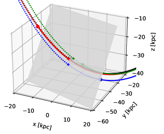
This leads to the second step of coordinate transformation, illustrated in Figure 16: each point in the 6d phase space gives rise to an orbit that crosses the fiducial hyperplane, and can be represented by the crossing point (coordinates in this 5d hyperplane) and the time of crossing. Unlike the first step, which was just a linear transformation effected by an orthogonal matrix, the second transformation is manifestly nonlinear, and is also not quite symmetric. The conversion from physical to scaled coordinates requires an entire orbit, not just a single point: we linearly transform the orbit into the rotated basis, determine the moment at which it crosses the fiducial hyperplane (i.e., when its first component in the rotated basis changes sign from negative to positive), and use the time offset between the actual point and the crossing point as the first coordinate , and the remaining five coordinates of the crossing point in the rotated basis as . The inverse transformation from scaled to physical space requires orbit integration from a point in the fiducial hyperplane specified by for a time , and can be carried out only approximately (because the equations of motion ignore the residual accelerations not described by the assumed combined potential ). Nevertheless, as long as is much shorter than dynamical time, this procedure remains sufficiently accurate to capture the primary source of nonlinearity (curvilinear trajectory in the potential ).
A.3 Iterative adjustment of orbital initial conditions
To determine the direction in which the orbital initial conditions should be adjusted, at each iteration we perform a series of simulations with slightly different initial conditions, find the deviations of each orbit in the series from the target 6d phase-space point (present-day position and velocity of the LMC), and then use the Newton method to determine the next initial conditions that will hopefully bring the simulated orbit closer to the target. The initial and final deviations are considered in the nonlinearly transformed coordinates, as described in the previous section.
Let be a matrix of initial conditions in the basis associated with the initial phase-space point of the master orbit, and be a matrix of the same size with the final (present-day) phase-space coordinates in the basis associated with the true position and velocity of the LMC. As described above, the first element of each column vector in the nonlinearly transformed coordinates is the time offset between the point and the fiducial 5d hyperplane of the given basis, while the remaining five elements are the usual coordinates in this fiducial hyperplane. The first column of the matrix corresponds to the master orbit and is therefore zero by construction, but the corresponding first column of the matrix is not necessarily so – in fact, making it zero is the goal of orbit finding. The usual assumption is that the mapping between the initial and the final conditions can be linearized in the vicinity of the master orbit, so that
for all companion orbits , where is the Jacobian of this mapping (which we also need to determine). This equality is only approximate for two reasons: first, a linearized form may not be valid for large displacements of companion orbits from the master one. Second, the final coordinates of orbits , including itself, are measured with some uncertainty due to stochastic nature of -body simulations. Therefore, the displacements of companion orbits should not be too small either, otherwise the Jacobian computed by subtracting final coordinates of nearby orbits will be dominated by noise. Because the master orbit is no better than others in terms of noisiness, it is advantageous to rewrite the above equation in terms of the deviation of all orbits from the target final coordinates (which are specified exactly – of course, in reality the measurement of the LMC position and velocity has some observational uncertainty, but the goal of this procedure is to drive different simulations exactly to the same final point for a fair comparison). In the full matrix form, it reads
where the elements of the row vector are ones, and the column vector replaces in the role of the final coordinates of the master orbit, and would coincide with it in the absence of noise. Both and elements of the Jacobian matrix are unknowns, and can be combined into a single matrix, while the matrix is augmented with an extra row consisting of ones. Transposing these matrices, we have
The first term on the left-hand side is a known design matrix of shape , the second term is the matrix of unknowns of shape , and the right-hand side is a matrix of shape , measured with some errors. This kind of problem is naturally solved by a linear least-square fit with the same design matrix, but multiple columns on the right-hand side providing solutions for corresponding columns of the matrix of unknowns. We need to be at least 7, but a larger number of equations (overdetermined fit) will improve robustness of the inferred Jacobian and the final displacement vector of the master orbit. In practice, we use two companion orbits with opposite displacements for each coordinate, i.e., .
After obtaining the solution for and , the next initial conditions are given by . However, if the Jacobian is ill-conditioned, the prescription for the next initial conditions may become quite unstable. This probably reflects a real physical degeneracy: one can make the initial orbital energy lower (case 1), or reduce its angular momentum while keeping energy fixed (case 2), and in the second case a smaller pericentre radius will create a stronger dynamical friction and cause the energy to drop faster, making the subsequent orbit very similar to case 1.
An alternative formulation deals with the vector of next initial conditions directly, writing the current initial conditions for all orbits as an inverse mapping from their final coordinates:
Now the matrix is augmented with an extra row of ones, while the vector is combined with the inverse Jacobian into the matrix of unknowns in the least-square fit:
The advantage of this approach is that the Jacobian is not used for inferring , effectively become a set of nuisance parameters; however, now the design matrix contains some noise, while the right-hand side is known perfectly, contrary to the assumptions of the least-square fit. Nevertheless, if the first procedure produces an unreasonable guess for the next initial conditions, we can use the more stable (even if generally less accurate) second formulation instead.
After the next initial conditions in the current basis are obtained, they are converted to physical coordinates by following the approximate equations of motion for the given time offset (the first element of the vector ), and then a new master orbit and a new set of companion orbits are started from that point, with a new associated basis for converting physical to scaled coordinates. The iterative procedure typically needs to be repeated 3–5 times, with the early stages using lower-resolution simulations to save time (but sacrifice accuracy of computing the Jacobian).