¹¹institutetext: Zhejiang University, Hangzhou, China
¹¹email: {shuaixie, zunleifeng, lynesychen, songtaosun, chaoma, brooksong}@zju.edu.cn

DEAL: Difficulty-aware Active Learning for Semantic Segmentation

Shuai Xie 11 Zunlei Feng 11 Ying Chen 11 Songtao Sun 11 Chao Ma 11 Mingli Song 11

Abstract

Active learning aims to address the paucity of labeled data by finding the most informative samples. However, when applying to semantic segmentation, existing methods ignore the segmentation difficulty of different semantic areas, which leads to poor performance on those hard semantic areas such as tiny or slender objects. To deal with this problem, we propose a semantic Difficulty-awarE Active Learning (DEAL) network composed of two branches: the common segmentation branch and the semantic difficulty branch. For the latter branch, with the supervision of segmentation error between the segmentation result and GT, a pixel-wise probability attention module is introduced to learn the semantic difficulty scores for different semantic areas. Finally, two acquisition functions are devised to select the most valuable samples with semantic difficulty. Competitive results on semantic segmentation benchmarks demonstrate that DEAL achieves state-of-the-art active learning performance and improves the performance of the hard semantic areas in particular.

Keywords:

Active learning Semantic segmentation Difficulty-aware

1 Introduction

Semantic segmentation is a fundamental task for various applications such as autonomous driving [1, 2], biomedical image analysis [3, 4, 5], remote sensing [6] and robot manipulation [7]. Recently, data-driven methods have achieved great success with large-scale datasets [8, 9]. However, tremendous annotation cost has become an obstacle for these methods to be widely applied in practical scenarios. Active Learning (AL) can be the right solution by finding the most informative samples. Annotating those selected samples can support sufficient supervision information and reduce the requirement of labeled samples dramatically.

Previous methods can be mainly categorized into two families: uncertainty-based [10, 11, 12, 13] and representation-based [14, 15, 16]. However, many works [10, 12, 14, 16] are only evaluated on image classification benchmarks. There has been considerably less work specially designed for semantic segmentation. Traditional uncertainty-based methods like Entropy [17] and Query-By-Committee (QBC) [18] have demonstrated their effectiveness in semantic segmentation [19, 20]. However, all of them are solely based on the uncertainty reflected on each pixel, without considering the semantic difficulty and the actual labeling scenarios.

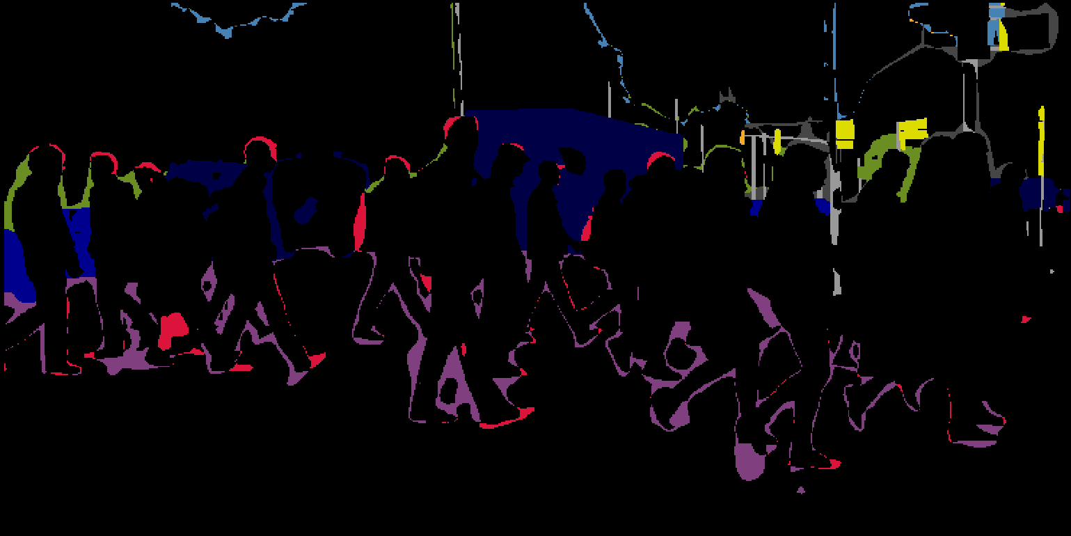
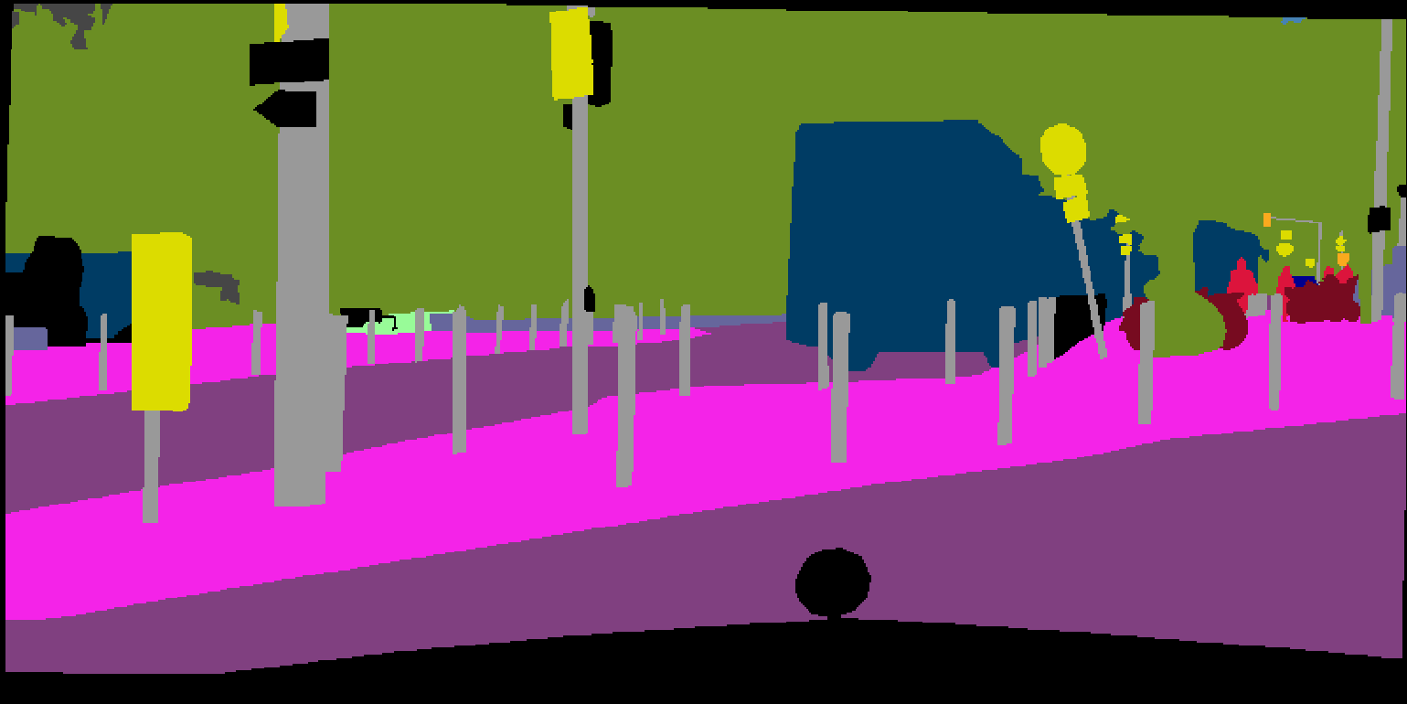
In this paper, we propose a semantic Difficulty-awarE Active Learning (DEAL) method taking the semantic difficulty into consideration. Due to the class imbalance and shape disparity, a noticeable semantic difficulty difference exists among the different semantic areas in an image. To capture this difference, we adopt a two-branch network composed of a semantic segmentation branch and a semantic difficulty branch. For the former branch, we adopt the common segmentation network. For the latter branch, we leverage the wrong predicted result as the supervision, which is termed as the error mask. It’s a binary image where the right and wrong positions have a value 0 and 1, respectively. As illustrated in Fig. 1(e), we color these wrong positions for better visualization. Then, a pixel-wise probability attention module is introduced to aggregate similar pixels into areas and learn the proportion of misclassified pixels as the difficulty score for each area. Finally, we can obtain the semantic difficulty map in Fig. 1(b).

Then two acquisition functions are devised based on the map. One is Difficulty-aware uncertainty Score (DS) combining the uncertainty and difficulty. The other is Difficulty-aware semantic Entropy (DE) solely based on the difficulty. Experiments show that the learned difficulty scores have a strong connection with the standard evaluation metric IoU. And DEAL can effectively improve the overall AL performance and the IoU of the hard semantic classes in particular.

In summary, our major contributions are as follows: 1) Proposing a new AL framework incorporating the semantic difficulty to select the most informative samples for semantic segmentation. 2) Utilizing error mask to learn the semantic difficulty. 3) Competitive results on CamVid [21] and Cityscapes [8].

2 Related Work

2.0.1 AL for semantic segmentation

The core of AL is measuring the informativeness of the unlabelled samples. Modern AL methods can be mainly divided into two groups: uncertainty-based [10, 11, 12, 13] and representation-based [14, 15, 16]. The latter views the AL process as an approximation of the entire data distribution and query samples to increase the data diversity, such as Core-set [14] and VAAL [15], which can be directly used in semantic segmentation. There are also some methods specially designed for semantic segmentation, which can also be divided into two groups: image-level [4, 11, 19, 22] and region-level [23, 24, 20].

Image-level methods use the complete image as the sampling unit. [4] propose suggestive annotation (SA) and train a group of models on various labeled sets obtained with bootstrap sampling and select samples with the highest variance. [11] employ MC dropout to measure uncertainty for melanoma segmentation. [19] adopt QBC strategy and propose a cost-sensitive active learning method for intracranial hemorrhage detection. [22] build a batch mode multi-clue method, incorporating edge information with QBC strategy and graph-based representativeness. All of them are based on a group of models and time-consuming when querying a large unlabeled data pool.

Region-level methods only sample the informative regions from images. [23] combines the MC dropout uncertainty with an effort estimation regressed from the annotation click patterns, which is hard to access for many datasets. [24] propose ViewAL and use the inconsistencies in model predictions across viewpoints to measure the uncertainty of super-pixels, which is specially designed for RGB-D data. [20] model a deep Q-network-based query network as a reinforcement learning agent, trying to learn sampling strategies based on prior AL experience. In this work, we incorporate the semantic difficulty to measure the informativeness and select samples at the image level. Region-level method will be studied in the future.

2.0.2 Self-attention mechanism for semantic segmentation

The self-attention mechanism is first proposed by [25] in the machine translation task. Now, it has been widely used in many tasks [25, 26, 27, 28] owing to its intuition, versatility and interpretability [29]. The ability to capture the long-range dependencies inspires many semantic segmentation works designing their attention modules. [30] use a point-wise spatial attention module to aggregate context information in a self-adaptive manner. [31] introduce an object context pooling scheme to better aggregate similar pixels belonging to the same object category. [32] replace the non-local operation [33] into two consecutive criss-cross operations and gather long-range contextual information in the horizontal and vertical directions. [34] design two types of attention modules to exploit the dependencies between pixels and channel maps. Our method also uses the pixel-wise positional attention mechanism in [34] to aggregate similar pixels.

3 Method

Before introducing our method, we first give the definition of the AL problem. Let $(x^{a},y^{a})$ be an annotated sample from the initial annotated dataset $\mathcal{D}^{a}$ and $x^{u}$ be an unlabeled sample from a much larger unlabeled data pool $\mathcal{D}^{u}$ . AL aims to iteratively query a subset $\mathcal{D}^{s}$ containing the most informative $m$ samples $\{x^{u}_{1},x^{u}_{2},...,x^{u}_{m}\}$ from $\mathcal{D}^{u}$ , where $m$ is a fixed budget.

In what follows, we first give an overview of our difficulty-aware active learning framework, then detail the probability attention module and loss functions, finally define two acquisition functions.

3.1 Difficulty-aware Active Learning

To learn the semantic difficulty, we exploit the error mask generated from the segmentation result. Our intuition is that these wrong predictions are what our model “feels” difficult to segment, which may have a relation with the semantic difficulty. Thus, we build a two-branch network generating semantic segmentation result and semantic difficulty map in a multi-task manner, best viewed in Fig. 2. The first branch is a common segmentation network, which can be used to generate the error mask. The second branch is devised to learn the semantic difficulty map with the guidance of error mask. This two-branch architecture is inspired by [13]. In their work, a loss prediction module is attached to the task model to predict a reliable loss for $x^{u}$ and samples with the highest losses are selected. While in our task, we dig deeper into the scene and analyze the semantic difficulty of each area.

As illustrated in Fig. 2, the first branch can be any semantic segmentation network. Assume $S^{*}$ is the output of softmax layer and $S^{p}$ is the prediction result after the argmax operation. With the segmentation result $S^{p}$ and GT $S^{g}$ , the error mask $M^{e}$ can be computed by:

\displaystyle M^{e}_{k}=\begin{cases}1&\text{if }S^{p}_{k}\neq S^{g}_{k},\\ 0&\text{otherwise},\end{cases}

(1)

where $S^{p}_{k}$ and $S^{g}_{k}$ denote the $k^{th}$ pixel value of the segmentation result and GT, $M^{e}_{k}$ is the $k^{th}$ pixel value of the error mask.

The second branch is composed of two parts: a probability attention module and a simple $1\times 1$ convolution layer used for binary classification. The softmax output of the first branch $S^{*}$ is directly used as the input of the second branch, which are $C$ -channel probability maps and $C$ is the number of classes. We denote it as $P\in\mathcal{R}^{C\times H\times W}$ and $P_{k}$ is the probability vector for the $k^{th}$ pixel. Using probability maps is naive but accompanied with two advantages. First, pixels with similar difficulty tend to have similar $P_{k}$ . Second, pixels of the same semantic tend to have similar $P_{k}$ . Combined with a pixel-wise attention module, we can easily aggregate these similar pixels and learn similar difficulty scores for them. In our learning schema, the performance of the second branch depends much on the output of the first branch. However, there is no much difference if we branch these two tasks earlier and learn the independent features. We validate this opinion in Sec. 5.2.

The semantic difficulty learning process can be imagined into two steps. Firstly, we learn a binary segmentation network with the supervision of error mask $M^{e}$ . Each pixel will learn a semantic difficulty score. Secondly, similar pixels are aggregated into an area so that this score can be spread among them. Finally, we can obtain the semantic difficulty map $M^{d}$ .

\begin{overpic}[width=433.62pt]{figs/overview.pdf} \put(2.2,32.2){$(x^{a},y^{a})$} \put(15.0,32.2){$x^{u}$} \put(5.0,25.0){$\mathcal{D}^{a}$} \put(15.0,25.0){$\mathcal{D}^{u}$} \put(11.0,8.0){$\mathcal{D}^{s}$} \par\put(8.0,13.5){$+$} \put(18.2,13.5){$-$} \par\put(61.0,37.0){$S^{*}$} \put(75.0,36.0){$S^{p}$} \put(91.2,36.0){$S^{g}$} \put(75.0,32.5){$M^{d}$} \put(91.0,32.5){$M^{e}$} \par\put(27.0,32.4){$P$} \put(53.0,32.4){$Q$} \par\put(81.5,43.7){$\mathcal{L}_{seg}$} \put(81.7,29.0){$\mathcal{L}_{dif}$} \end{overpic}

Figure 2: Overview of our difficulty-aware active learning framework for semantic segmentation. The first branch is a common semantic segmentation network. The second branch is composed of a praobability attention module and a

1\times 1

convolution.

\mathcal{D}^{a}

and

\mathcal{D}^{u}

are the annotated and unlabeled data,

\mathcal{D}^{s}

is a subset selected from

\mathcal{D}^{u}

P

and

Q

are the probability maps before and after attention.

\mathcal{L}_{seg}

and

\mathcal{L}_{dif}

are the loss functions described in Eq. 3 and Eq. 4. DS and DE strategies are detailed in Sec. 3.4.

3.2 Probability Attention Module

In this section, we detail the probability attention module (PAM) in our task. Inspired by [34], we use this module to aggregate pixels with similar softmax probability. Given the probability maps $P\in\mathcal{R}^{C\times H\times W}$ , we first reshape it to $P\in\mathcal{R}^{C\times K}$ , where $K=H\times W$ . Then the probability attention matrix $A\in\mathcal{R}^{K\times K}$ can be computed with $P^{T}P$ and a softmax operation as below:

\displaystyle\begin{split}A_{ji}&=\frac{exp(P^{T}_{i}\cdot P_{j})}{\sum_{i=1}^{K}exp(P^{T}_{i}\cdot P_{j})},\\ Q_{j}&=\gamma\sum_{i=1}^{K}(A_{ji}P_{i})+P_{j},\end{split}

(2)

where $A_{ji}$ is the $i^{th}$ pixel’s impact on $j^{th}$ pixel, $P_{j}$ is the original probability vector of the $j^{th}$ pixel and $Q_{j}$ is the one after attention, $\gamma$ is a learnable weight factor. Finally, we can get the probability maps $Q\in\mathcal{R}^{C\times H\times W}$ after attention.

Let’s take the segmentation result of the two bicyclists in Fig. 2 to explain the role of PAM as it reflects two typical errors in semantic segmentation: (1) error inside the object (the smaller one $b_{1}$ ); (2) error on the object boundary (the larger one $b_{2}$ ), as shown in Fig. 3. Assume our attention module can aggregate pixels from the same object together, the right part of the object learns 0 while the wrong part learns 1. Since $b_{1}$ has a larger part of wrong areas, it tends to learn larger difficulty scores than $b_{2}$ . Similar to objects, pixels from the same semantic, such as road, sky and buildings can also learn similar difficulty scores. Ablation study in Sec. 5.1 also demonstrates that PAM can learn more smooth difficulty scores for various semantic areas.

Some traditional methods also employ the softmax probabilities to measure the uncertainty, such as least confidence (LC) [35], margin sampling (MS) [36] and Entropy [17]. The most significant difference between our method and these methods is that we consider difficulty at the semantic level with an attention module, rather than measuring the uncertainty of each pixel alone. QBC [18] can use a group of models, but it still stays at the pixel level. To clearly see the difference, we compare our semantic difficulty map with the uncertainty maps of these methods in Fig. 4. The first row are uncertainty maps generated with these methods, which are loyal to the uncertainty of each pixel. For example, some pixels belonging to sky can have the same uncertainty with traffic light and traffic sign. Supposing an image has many pixels with high uncertainty belonging to the easier classes, it will be selected by these methods. While our semantic difficulty map (first in the second row) can serve as the difficulty attention and distinguish more valuable pixels. As illustrated in the second row, combined with our difficulty map, the uncertainty of the easier semantic areas like sky is suppressed while the harder semantic areas like traffic sign is reserved.

3.3 Loss Functions

3.3.1 Loss of Semantic Segmentation

To make an equitable comparison with other methods, we use the standard cross-entropy loss for the semantic segmentation branch, which is defined as:

\displaystyle\mathcal{L}_{seg}(S^{*},S^{g})=\frac{1}{K}\sum^{K}_{k=1}\mathcal{\ell}(S_{k}^{*},S_{k}^{g})+R(\theta),

(3)

where $S_{k}^{*}$ and $S_{k}^{g}$ are the segmentation output and ground truth for pixel $k$ , $\mathcal{\ell}(\cdot)$ is the cross-entropy loss, $K$ is the total pixel number, and $R$ is the L2-norm regularization term.

3.3.2 Loss of Semantic Difficulty

For the semantic difficulty branch, we use an inverted weighted binary cross-entropy loss defined below, as there is a considerable imbalance between the right and wrong areas of error mask.

\displaystyle\begin{split}\mathcal{L}_{dif}(M^{d},M^{e})=-&\frac{1}{K}\sum_{k=1}^{K}\lambda_{1}M_{k}^{e}log(M_{k}^{d})+\lambda_{2}(1-M_{k}^{e})log(1-M_{k}^{d}),\\ &\lambda_{1}=\frac{\sum_{k}^{K}\mathbf{1}(M_{k}^{e}=0)}{K},\lambda_{2}=1-\lambda_{1},\end{split}

(4)

where $M_{k}^{d}$ and $M_{k}^{e}$ are the difficulty prediction and error mask ground truth for pixel $k$ , $\mathbf{1(\cdot)}$ is the indicator function, and $\lambda_{1}$ and $\lambda_{2}$ are dynamic weight factors.

3.3.3 Final Loss

Our final training objective is a combination of Eq. 3 and Eq. 4, which is computed as:

\displaystyle\mathcal{L}=\mathcal{L}_{seg}+\alpha\mathcal{L}_{dif},

(5)

where $\alpha$ is a weight factor and set to 1 in the experiments.

3.4 Acquisition Functions

Samples from $\mathcal{D}^{u}$ are usually ranked with a scalar score in AL. However, semantic segmentation is a dense-classification task, many methods output a score for each pixel on the image, including our semantic difficulty map. Thus, it’s quite significant to design a proper acquisition function. Below are two functions we have designed.

3.4.1 Difficulty-aware uncertainty Score (DS)

Assume $M^{c}$ is the uncertainty map generated with traditional methods like Entropy, we can define the equation below to make each pixel aware of its semantic difficulty.

\displaystyle\mathcal{S}_{DS}=\frac{1}{K}\sum^{K}_{k=1}M^{c}_{k}\cdot M_{k}^{d},

(6)

where $M^{c}_{k}$ and $M^{d}_{k}$ are the uncertainty score and difficulty score of the $k^{th}$ pixel, $K$ is the total pixel number, $\mathcal{S}_{DS}$ is the average difficulty-aware uncertainty score for selecting samples with the highest uncertainty.

3.4.2 Difficulty-aware semantic Entropy (DE)

This acquisition function is inspired by the laddered semantic difficulty reflected on $M^{d}$ . Usually, pixels from the same semantic area have almost the same semantic difficulty scores, best viewed in Fig. 5(c). In this example, we quantify the difficulty of pixels in Fig. 5(a) into 6 levels in Fig. 5(d-i), with difficulty scores gradually increasing from level 1 to level 6. Generally, if we quantify the difficulty in an image into $L$ levels, the difficulty entropy acquisition function can be defined below to query samples with more balanced semantic difficulty, which can be viewed as a representation-based method at the image scale.

\displaystyle\mathcal{S}_{DE}=-\sum_{l=1}^{l=L}\frac{K_{l}}{K}log(\frac{K_{l}}{K}),

(7)

where $K_{l}$ is the number of pixels falling in the $l^{th}$ difficulty level, $K$ is the total pixel number, $L$ is the quantified difficulty levels, $\mathcal{S}_{DE}$ is the difficulty-aware semantic entropy for selecting samples with more balanced semantic difficulty. Our full algorithm of DEAL is shown in Algorithm 1.

\mathcal{D}^{a}

\mathcal{D}^{u}

, budget

m

, AL query times

N

, initialized network parameter

\Theta

0: iterations

T

, weight factor

\alpha

, quantified difficulty levels

L

(optional)

\mathcal{D}^{a}

\mathcal{D}^{u}

, Optimized

\Theta

1: for

n=1,2,...,N

2: Train the two-branch difficulty learning network on

\mathcal{D}^{a}

3: for

t=1,2,...,T

4: Sample

(x^{a},y^{a})

from

\mathcal{D}^{a}

5: Compute the segmentation output

S^{*}

and result

S^{p}

6: Obtain

M^{e}

according to Eq. 1

7: Compute the difficulty prediction

M^{d}

8: Compute

\mathcal{L}_{seg}

\mathcal{L}_{dif}

\mathcal{L}

according to Eq. 3, Eq. 4, Eq. 5

9: Update

\Theta

using gradient descent

10: end for

11: Rank

x^{u}

based on Eq. 6 or Eq. 7

12: Select

\mathcal{D}^{s}

with top

m

samples

13: Annotate

\mathcal{D}^{s}

by oralces

14:

\mathcal{D}^{a}\leftarrow\mathcal{D}^{a}+\mathcal{D}^{s}

15:

\mathcal{D}^{u}\leftarrow\mathcal{D}^{u}-\mathcal{D}^{s}

16: end for

17: return

\mathcal{D}^{a}

\mathcal{D}^{u}

, Optimized

\Theta

Algorithm 1 Difficulty-aware Active Learning Algorithm

4 Experiments and Results

In this section, we first describe the datasets we use to evaluate our method and the implementation details, then the baseline methods, finally compare our results with these baselines.

Table 1: Evaluation datasets.

Dataset	Classes	Train	Valid	Test	Initial labeled	Budget	Image Size
CamVid [21]	11	370	104	234	40	20	$360\times 480$
Cityscapes [8]	19	2675	300	500	300	150	$688\times 688$

4.1 Experimental Setup

4.1.1 Datasets

We evaluate DEAL on two street scene semantic segmentation datasets: CamVid [21] and Cityscapes [8]. For Cityscapes, we randomly select 300 samples from the training set as the validation set, and the original validation set serves as the test set, same to [15]. The detailed configurations are list in Table 1. For each dataset, we first randomly sample $10\%$ data from the training set as the initial annotated dataset $\mathcal{D}^{a}$ , then iteratively query $5\%$ new data $\mathcal{D}^{s}$ from the remaining training set, which serves as the unlabeled data pool $\mathcal{D}^{u}$ . Considering samples in the street scenes have high similarities, we first randomly choose a subset from $\mathcal{D}^{u}$ , then query $m$ samples from the subset, same to [37].

4.1.2 Implementation Details

We adopt the Deeplabv3+ [38] architecture with a Mobilenetv2 [39] backbone. For each dataset, we use mini-batch SGD [40] with momentum 0.9 and weight decay $5e^{-4}$ in training. The batch size is 4 and 8 for CamVid and Cityscapes, respectively. For all methods and the upper bound method with the full training data, we train 100 epochs with an unweighted cross-entropy loss function. Similar to [38], we apply the “poly” learning rate strategy and the initial learning rate is 0.01 and multiplied by $(1-\frac{iter}{max\_iter})^{0.9}$ . To accelerate the calculation of the probability attention module, the input of the difficulty branch is resized to $80\times 60$ and $86\times 86$ for CamVid and Cityscapes.

4.2 Evaluated Methods

We compare DEAL with the following methods. Random is a simple baseline method. Entropy and QBC are two uncertainty-based methods. Core-set and VAAL are two representation-based methods. DEAL (DS) and DEAL (DE) are our methods with different acquisition functions.

•

Random: each sample in $\mathcal{D}^{u}$ is queried with uniform probability.
•

Entropy (Uncertainty): we query samples with max mean entropy of all pixels. [13] and [20] have verified this method is quite competitive in image classification and segmentation tasks.
•

QBC (Uncertainty): previous methods designed for semantic segmentation, like [4, 11, 22, 23], all use a group of models to measure uncertainty. We use the efficient MC dropout to represent these methods and report the best performance out of both the max-entropy and variation-ratio acquisition functions.
•

Core-set (Representation): we query samples that can best cover the entire data distribution. We use the global average pooling operation on the encoder output features of Deeplabv3+ and get a feature vector for each sample. Then k-Center-Greedy strategy is used to query the most informative samples, and the distance metric is $l_{2}$ distance according to [14].
•

VAAL (Representation): as a new state-of-the-art task-agnostic method, the sample query process of VAAL is totally separated from the task learner. We use this method to query samples that are most likely from $\mathcal{D}^{u}$ and then report the performance with our task model.
•

DEAL (DS): out method with DS acquisition function. We employ Entropy uncertainty maps in our experiments.
•

DEAL (DE): out method with DE acquisition function. The quantified difficulty levels $L$ are set 8 and 10 for CamVid and Cityscapes, respectively.

4.3 Experimental Results

The mean Intersection over Union (mIoU) at each AL stage: 10%, 15%, 20%, 25%, 30%, 35%, 40% of the full training set, are adopted as the evaluation metric. Every method is run 5 times and the average mIoUs are reported.

4.3.1 Results on CamVid

Fig. 6(a) shows results on a small dataset CamVid. Both DEAL (DS) and DEAL (DE) outperform baseline methods at each AL stage. We can obtain a performance of 61.64% mIoU with 40% training data, about 95% of the upper performance with full training data. Entropy can achieve good results at the last stage. However, it’s quite unstable and depends much on the performance of current model, making it behave poorly and exceeded by Random at some stages. On the contrary, DEAL (DS) behaves better with the difficulty attention. QBC has a more stable growth curve as it depends less on the single model. Representation-based methods like VAAL and Core-set behave much better at earlier stages like 15% and 20%. However, Core-set lags behind later while VAAL still works well. Also, the experiment results suggest that the data diversity is more important when the entire dataset is small.

4.3.2 Results on Cityscapes

Fig. 6(b) shows results on a larger dataset Cityscapes. The budget is 150 and all methods have more stable growth curves. When the budget is enough, Entropy can achieve better performance than other baseline methods. Consistently, with semantic difficulty, both DEAL (DS) and DEAL (DE) outperform other methods. Table 2 shows the per-class IoU for each method at the last AL stage (40% training data). Compared with Entropy, our method are more competitive on the difficult classes, such as pole, traffic sign, rider and motorcycle. For representation-based methods, the gap between Core-set and VAAL is more obvious, suggesting that Core-set is less effective when the input has a higher dimension. And VAAL is easily affected by the performance of the learned variational autoencoder, which introduces more uncertainty to the active learning system. If continue querying new data, our method will reach the upper performance of full training data with about 60% data.

Table 2: Per-class IoU of and mIoU [%] on Cityscapes original validation set with 40% training data. For clarity, only the average of 5 runs are reported, and the best and the second best results are highlighted in bold and underline bold.

Method	Road	Side-walk	Build-ing	Wall	Fence	Pole	Traffic Light	Traffic Sign	Vege-tation	Terrain
Random	96.03	72.36	86.79	43.56	44.22	36.99	35.28	53.87	86.91	54.58
Core-set	96.12	72.76	87.03	44.86	45.86	35.84	34.81	53.07	87.18	53.49
VAAL	96.22	73.27	86.95	47.27	43.92	37.40	36.88	54.90	87.10	54.48
QBC	96.07	72.27	87.05	46.89	44.89	37.21	37.57	54.53	87.51	55.13
Entropy	96.28	73.31	87.13	43.82	43.87	38.10	37.74	55.39	87.52	53.68
DEAL (DS)	96.21	72.72	86.94	46.11	44.22	38.18	37.62	55.66	87.34	55.62
DEAL (DE)	95.89	71.69	87.09	45.61	44.94	38.29	36.51	55.47	87.53	56.90
	Sky	Pedes-trian	Rider	Car	Truck	Bus	Train	Motor-cycle	Bicycle	mIoU
Random	91.47	62.74	37.51	88.05	54.64	61.00	43.69	30.58	55.67	59.79
Core-set	91.89	62.48	36.28	87.63	57.25	67.02	56.59	29.34	53.56	60.69
VAAL	91.63	63.44	38.92	87.92	50.15	63.70	52.36	35.99	54.97	60.92
QBC	91.87	63.79	38.76	88.04	53.88	65.92	54.32	32.68	56.15	61.29
Entropy	92.05	63.96	38.44	88.38	59.38	64.64	50.80	36.13	57.10	61.46
DEAL (DS)	92.10	63.92	40.39	87.87	59.85	67.32	52.30	38.88	55.44	62.04
DEAL (DE)	91.78	64.25	39.77	88.11	56.87	64.46	50.39	38.92	56.69	61.64

5 Ablation Study

5.1 Effect of PAM

\begin{overpic}[width=433.62pt]{figs/att.pdf} \put(4.0,0.0){ (a) GT} \put(16.0,0.0){ (b) Prediction} \put(32.5,0.0){ (c) Error mask} \put(49.0,0.0){ (d) Attention 1} \put(66.0,0.0){ (e) Attention 2} \put(83.0,0.0){ (f) Attention 3} \end{overpic}

Figure 7: Attention heatmaps of three selected wrong predicted pixels on CamVid [21]. (a) GT. (b) Prediction. (c) Error mask. (d,e,f) Attention heatmaps of the three selected points, which are marked as {1,2,3} in (a,b,c). The warmer color means the more dependency.

To further understand the effect of PAM, we first visualize the attention heatmaps of the wrong predictions in Fig. 7. For each row, three points are selected from error mask and marked as $\{1,2,3\}$ in Fig. 7(a,b,c). In the first row, point 1 is from road and misclassified as bicyclist, we can observe that its related classes are bicyclist, road and sidewalk in Fig. 7(d). Point 2 is from buildings and misclassified as bicyclist, too. Point 3 is from sign symbol and misclassified as tree, we can also observe its related semantic areas in Fig. 7(f).

Then we conduct an ablation study by removing PAM and directly learning the semantic difficulty map without the attention among pixels. The qualitative results are shown in Fig. 8(a). Basically, without the long-range dependencies, pixels of the same semantic can learn quite different scores because the learned score of each pixel is more sensitive to its original uncertainty. Combined with PAM, we can learn more smooth difficulty map, which is more friendly to the annotators since the aggregated semantic areas are close to the labeling units in the real scenario. Also, we compare this ablation model with our original model on Cityscapes in Fig. 8 (b). DEAL with PAM can achieve a better performance at each AL stage. DEAL without PAM fails to find samples with more balanced semantic difficulty, which makes it get a lower entropy of class distributions.

5.2 Branch Position

In this section, we discuss the branch position of our framework. In our method above, the semantic difficulty branch is simply added after the segmentation branch. It may occur to us that if the segmentation branch performs poorly, the difficulty branch will perform poorly, too. These two tasks should be separated earlier and learn independent features. Thus, we modify our model architecture and branch out two tasks earlier at the boarder of encoder and decoder based on the Deeplabv3+[38] architecture, as shown in Fig. 9(a). Also, we compare the AL performance on Cityscapes with both architectures in Fig. 9(b). The performance of the modified version is slightly poor than the original version but still competitive with other methods. However, this modified version requires more computations, while our original version is simple yet effective and can be easily plugged into any segmentation networks.

6 Conclusion and Future Work

In this work, we have introduced a novel Difficulty-awarE Active Learning (DEAL) method for semantic segmentation, which incorporates the semantic difficulty to select the most informative samples. For any segmentation network, the error mask is firstly generated with the predicted segmentation result and GT. Then, with the guidance of error mask, the probability attention module is introduced to aggregate similar pixels and predict the semantic difficulty maps. Finally, two acquisition functions are devised. One is combining the uncertainty of segmentation result and the semantic difficulty. The other is solely based on the difficulty. Experiments on CamVid and Cityscapes demonstrate that the proposed DEAL achieves SOTA performance and can effectively improve the performance of hard semantic areas. In the future work, we will explore more possibilities with the semantic difficulty map and apply it to region-level active learning method for semantic segmentation.

7 Acknowledgments

This work is funded by National Key Research and Development Project (Grant No: 2018AAA0101503) and State Grid Corporation of China Scientific and Technology Project: Fundamental Theory of Human-in-the-loop Hybrid-Augmented Intelligence for Power Grid Dispatch and Control.

References

[1] Teichmann, M., Weber, M., Zoellner, M., Cipolla, R., Urtasun, R.: Multinet: Real-time joint semantic reasoning for autonomous driving. In: IEEE Intelligent Vehicles Symposium (IV). (2018) 1013–1020
[2] Feng, D., Haase-Schütz, C., Rosenbaum, L., Hertlein, H., Glaeser, C., Timm, F., Wiesbeck, W., Dietmayer, K.: Deep multi-modal object detection and semantic segmentation for autonomous driving: Datasets, methods, and challenges. IEEE Transactions on Intelligent Transportation Systems (ITS) (2020)
[3] Ronneberger, O., Fischer, P., Brox, T.: U-net: Convolutional networks for biomedical image segmentation. In: International Conference on Medical Image Computing and Computer-Assisted Intervention (MICCAI), Springer (2015) 234–241
[4] Yang, L., Zhang, Y., Chen, J., Zhang, S., Chen, D.Z.: Suggestive annotation: A deep active learning framework for biomedical image segmentation. In: International Conference on Medical Image Computing and Computer-Assisted Intervention (MICCAI), Springer (2017) 399–407
[5] Zheng, H., Zhang, Y., Yang, L., Liang, P., Zhao, Z., Wang, C., Chen, D.Z.: A new ensemble learning framework for 3d biomedical image segmentation. In: Proceedings of the AAAI Conference on Artificial Intelligence (AAAI). Volume 33. (2019) 5909–5916
[6] Azimi, S.M., Henry, C., Sommer, L., Schumann, A., Vig, E.: Skyscapes fine-grained semantic understanding of aerial scenes. In: Proceedings of the IEEE International Conference on Computer Vision (ICCV). (2019) 7393–7403
[7] Puang, E.Y., Lehner, P., Marton, Z.C., Durner, M., Triebel, R., Albu-Schäffer, A.: Visual repetition sampling for robot manipulation planning. In: International Conference on Robotics and Automation (ICRA). (2019) 9236–9242
[8] Cordts, M., Omran, M., Ramos, S., Rehfeld, T., Enzweiler, M., Benenson, R., Franke, U., Roth, S., Schiele, B.: The cityscapes dataset for semantic urban scene understanding. In: Proceedings of the IEEE Conference on Computer Vision and Pattern Recognition (CVPR). (2016) 3213–3223
[9] Zhou, B., Zhao, H., Puig, X., Fidler, S., Barriuso, A., Torralba, A.: Scene parsing through ade20k dataset. In: Proceedings of the IEEE Conference on Computer Vision and Pattern Recognition (CVPR). (2017) 633–641
[10] Wang, K., Zhang, D., Li, Y., Zhang, R., Lin, L.: Cost-effective active learning for deep image classification. IEEE Transactions on Circuits and Systems for Video Technology (CSVT) 27 (2016) 2591–2600
[11] Gorriz, M., Carlier, A., Faure, E., Giro-i Nieto, X.: Cost-effective active learning for melanoma segmentation. In: Workshop of Advances in Neural Information Processing Systems. (2017)
[12] Gal, Y., Islam, R., Ghahramani, Z.: Deep bayesian active learning with image data. In: Proceedings of the International Conference on Machine Learning (ICML). (2017) 1183–1192
[13] Yoo, D., Kweon, I.S.: Learning loss for active learning. In: Proceedings of the IEEE Conference on Computer Vision and Pattern Recognition (CVPR). (2019) 93–102
[14] Sener, O., Savarese, S.: Active learning for convolutional neural networks: A core-set approach. In: International Conference on Learning Representations (ICLR). (2017)
[15] Sinha, S., Ebrahimi, S., Darrell, T.: Variational adversarial active learning. In: Proceedings of the IEEE International Conference on Computer Vision (ICCV). (2019) 5972–5981
[16] Gissin, D., Shalev-Shwartz, S.: Discriminative active learning. arXiv preprint arXiv:1907.06347 (2019)
[17] Shannon, C.E.: A mathematical theory of communication. Bell system technical journal 27 (1948) 379–423
[18] Seung, H.S., Opper, M., Sompolinsky, H.: Query by committee. In: Workshop on Computational learning theory. (1992) 287–294
[19] Kuo, W., Häne, C., Yuh, E., Mukherjee, P., Malik, J.: Cost-sensitive active learning for intracranial hemorrhage detection. In: International Conference on Medical Image Computing and Computer-Assisted Intervention (MICCAI), Springer (2018) 715–723
[20] Casanova, A., Pinheiro, P.O., Rostamzadeh, N., Pal, C.J.: Reinforced active learning for image segmentation. In: International Conference on Learning Representations (ICLR). (2020)
[21] Brostow, G.J., Fauqueur, J., Cipolla, R.: Semantic object classes in video: A high-definition ground truth database. Pattern Recognition Letters 30 (2009) 88–97
[22] Tan, Y., Yang, L., Hu, Q., Du, Z.: Batch mode active learning for semantic segmentation based on multi-clue sample selection. In: Proceedings of the ACM International Conference on Information and Knowledge Management (CIKM). (2019) 831–840
[23] Mackowiak, R., Lenz, P., Ghori, O., Diego, F., Lange, O., Rother, C.: Cereals: cost-effective region-based active learning for semantic segmentation. In: British Machine Vision Conference (BMVC). (2018)
[24] Siddiqui, Y., Valentin, J., Nießner, M.: Viewal: Active learning with viewpoint entropy for semantic segmentation. In: Proceedings of the IEEE Conference on Computer Vision and Pattern Recognition (CVPR). (2020) 9433–9443
[25] Vaswani, A., Shazeer, N., Parmar, N., Uszkoreit, J., Jones, L., Gomez, A.N., Kaiser, Ł., Polosukhin, I.: Attention is all you need. In: Advances in neural information processing systems (NeurIPS). (2017) 5998–6008
[26] Lin, Z., Feng, M., dos Santos, C.N., Yu, M., Xiang, B., Zhou, B., Bengio, Y.: A structured self-attentive sentence embedding. In: International Conference on Learning Representations (ICLR). (2017)
[27] Wang, Y., Huang, M., Zhu, X., Zhao, L.: Attention-based lstm for aspect-level sentiment classification. In: Proceedings of Conference on Empirical Methods in Natural Language Processing (EMNLP). (2016) 606–615
[28] Zhou, C., Bai, J., Song, J., Liu, X., Zhao, Z., Chen, X., Gao, J.: Atrank: An attention-based user behavior modeling framework for recommendation. In: Proceedings of the AAAI Conference on Artificial Intelligence (AAAI). (2018)
[29] Chaudhari, S., Polatkan, G., Ramanath, R., Mithal, V.: An attentive survey of attention models. ArXiv abs/1904.02874 (2019)
[30] Zhao, H., Zhang, Y., Liu, S., Shi, J., Change Loy, C., Lin, D., Jia, J.: Psanet: Point-wise spatial attention network for scene parsing. In: European Conference on Computer Vision (ECCV). (2018) 267–283
[31] Yuan, Y., Wang, J.: Ocnet: Object context network for scene parsing. arXiv preprint arXiv:1809.00916 (2018)
[32] Huang, Z., Wang, X., Huang, L., Huang, C., Wei, Y., Liu, W.: Ccnet: Criss-cross attention for semantic segmentation. Proceedings of the IEEE International Conference on Computer Vision (ICCV) (2019) 603–612
[33] Wang, X., Girshick, R.B., Gupta, A., He, K.: Non-local neural networks. IEEE Conference on Computer Vision and Pattern Recognition (CVPR) (2018) 7794–7803
[34] Fu, J., Liu, J., Tian, H., Li, Y., Bao, Y., Fang, Z., Lu, H.: Dual attention network for scene segmentation. In: Proceedings of the IEEE Conference on Computer Vision and Pattern Recognition (CVPR). (2019) 3146–3154
[35] Settles, B.: Active learning literature survey. Technical report, University of Wisconsin-Madison Department of Computer Sciences (2009)
[36] Scheffer, T., Decomain, C., Wrobel, S.: Active hidden markov models for information extraction. In: International Symposium on Intelligent Data Analysis (IDA), Springer (2001) 309–318
[37] Beluch, W.H., Genewein, T., Nürnberger, A., Köhler, J.M.: The power of ensembles for active learning in image classification. In: Proceedings of the IEEE Conference on Computer Vision and Pattern Recognition (CVPR). (2018) 9368–9377
[38] Chen, L.C., Zhu, Y., Papandreou, G., Schroff, F., Adam, H.: Encoder-decoder with atrous separable convolution for semantic image segmentation. In: European conference on computer vision (ECCV). (2018) 801–818
[39] Sandler, M., Howard, A., Zhu, M., Zhmoginov, A., Chen, L.C.: Mobilenetv2: Inverted residuals and linear bottlenecks. In: Proceedings of the IEEE Conference on Computer Vision and Pattern Recognition (CVPR). (2018) 4510–4520
[40] Krizhevsky, A., Sutskever, I., Hinton, G.E.: Imagenet classification with deep convolutional neural networks. In: Advances in Neural Information Processing Systems (NeurIPS). (2012) 1097–1105