Data Summarization via Bilevel Optimization
Abstract
The increasing availability of massive data sets poses a series of challenges for machine learning. Prominent among these is the need to learn models under hardware or human resource constraints. In such resource-constrained settings, a simple yet powerful approach is to operate on small subsets of the data. Coresets are weighted subsets of the data that provide approximation guarantees for the optimization objective. However, existing coreset constructions are highly model-specific and are limited to simple models such as linear regression, logistic regression, and -means. In this work, we propose a generic coreset construction framework that formulates the coreset selection as a cardinality-constrained bilevel optimization problem. In contrast to existing approaches, our framework does not require model-specific adaptations and applies to any twice differentiable model, including neural networks. We show the effectiveness of our framework for a wide range of models in various settings, including training non-convex models online and batch active learning.
Keywords: data summarization, coresets, bilevel optimization, continual learning, batch active learning
1 Introduction
Learning models on massive data sets faces several challenges. From a computational perspective, specific hardware resource constraints must be met: the data is first loaded into the system’s main memory with limited capacity, then it is processed by algorithms with possibly superlinear space or time complexity. Moreover, commonly used specialized hardware for accelerating data processing, such as GPUs, introduces another layer of constraints due to their limited memory. A simple yet powerful approach for tackling these computational challenges is to operate on small subsets of the data sampled uniformly at random—this idea is key to the success of stochastic optimization. However, real-world settings often involve rare but essential events with a significant impact on the optimization objective that are unlikely to be represented in a small uniform summary—a drawback that can be remedied by constructing a more representative summary.
Some settings face human resource constraints. A prominent example of such a setting is batch active learning, where the human expert is responsible for providing labels for the selected batch of points in each round of active learning. The cost and the limited availability of human attention impose explicit constraints on the number of points that can be labeled, accentuating the importance of compact and informative summaries.
Coresets are weighted subsets of the data that provide approximation guarantees for the optimization objective—the strongest form of these are uniform multiplicative guarantees. On the one hand, coresets with uniform approximation guarantees are a versatile tool for obtaining provably good solutions for optimization problems on massive data sets in batch, distributed, and streaming settings. On the other hand, such strong approximation guarantees are hard or even impossible to obtain for practical coreset sizes for some relevant problems. Consequently, coresets with uniform approximation guarantees are limited to simple models such as linear regression, logistic regression, -means, and Gaussian mixture models.
Moreover, existing coreset construction strategies are either model-specific or require model-specific derivations for instantiating their construction. For example, the popular framework of Feldman and Langberg (2011) for constructing coresets with uniform approximation guarantees relies on importance sampling based on upper bounds on the sensitivity of data points; the derivation of non-vacuous sensitivity upper bounds is a difficult model-specific task. While several alternative coreset definitions have been proposed, no principled coreset construction has been shown to succeed for a wide range of models. Moreover, coresets remain underexplored in practically relevant settings that rely on data summarization, including batch active learning, compression, and the training of non-convex models online, in spite of coresets being natural candidates for these settings.
In this work, we propose a generic coreset construction framework for twice differentiable models. We show that our method is effective for a wide range of models in various resource-constrained settings. In particular:
-
•
We formulate the coreset construction as a cardinality-constrained bilevel optimization problem that we solve by greedy forward selection and first-order methods. In contrast to existing coreset constructions, our framework applies to any twice differentiable model and does not require model-specific modifications.
-
•
We point out connections to robust statistics and experimental design, present theoretical guarantees for our framework and offer several variants for improved scalability. We discuss various extensions, including generating joint coresets for multiple models.
-
•
We demonstrate the advantage of our framework over other data summarization techniques in extensive experimental studies, over a wide range of models and resource-constrained settings, such as continual learning, streaming and batch active learning.
This work is a significant extension of Borsos et al. (2020) that demonstrated the effectiveness of the framework for building small coresets for neural networks with proxy models only. We extend the framework to constructing large coresets directly for the target models by proposing several variants of the basic algorithm. We demonstrate the effectiveness of our approach for models with millions of parameters, including wide residual networks, for which we show that we can compress CIFAR-10 by a factor of 2 and SVHN by a factor of 3 with less than loss of test accuracy. Furthermore, we offer several extensions to our framework, including constructing joint coresets for multiple models and dictionary selection for compressed sensing. The batch active learning application presented in this work is based on Borsos et al. (2021) with significant performance improvements.
2 Background and Related Work
In this section, we present relevant works on coresets and other data summarization techniques. The list of presented approaches is by no means exhaustive—we refer to Har-peled (2011); Phillips (2016); Bachem et al. (2017); Feldman (2020) for surveys about the topic.
Coresets are commonly defined as weighted subsets of the data. The types of theoretical guarantees provided by coresets, however, vary significantly. Consequently, a wide range of coresets construction algorithms have been proposed, the vast majority of which are applicable to a specific model only. The most common type of guarantees for coresets are uniform multiplicative approximation guarantees: for a given family of nonnegative real functions on the space , we want to find the coreset as the subset of the data and the associated weights such that for , holds with probability uniformly for all —we refer to coresets with such guarantees as -coresets.
Earliest approaches for constructing -coresets appear in computational geometry (Agarwal et al., 2005) and rely on exponential grids (Har-Peled and Mazumdar, 2004). Feldman and Langberg (2011) provide a unified -coreset-construction framework based importance sampling via the data points’ sensitivity (Langberg and Schulman, 2010). While efficient and effective for several models such as -median (Feldman and Langberg, 2011), logistic regression (Huggins et al., 2016), and Gaussian mixture models (Lucic et al., 2017), this framework relies bounding the sensitivity, which is a nontrivial, model-specific task. Moreover, the required coreset size depends also on the pseudo-dimension of the function class , limiting the framework to low-complexity models (compared to the number of points ).
Closely related to our work are coresets that require guarantees only with respect to the optimal solution on coreset instead of uniform guarantees. The majority of constructions providing such guarantees are deterministic (in contrast to the sampling-based sensitivity-framework): Badoiu and Clarkson (2003) provide a greedy forward selection of coresets for the minimum enclosing ball problem of size independent of both and ; based on the latter, Tsang et al. (2005) propose the Core Vector Machine, which selects a superset of support vectors for SVM in linear time, in a forward greedy manner. Clarkson (2010) points out that these approaches are instances of the Frank-Wolfe algorithm (Frank and Wolfe, 1956). When evaluating the optimal solution found on the coreset (in the unweighted case) on the full data, Wei et al. (2015) show that the resulting set function is submodular in the case of nearest neighbors and naive Bayes, hence greedy selection based on marginal gains guarantees a approximation factor to the cost of the solution on the best coreset of a given size. Similarly to the case of -coresets, existing deterministic coreset construction algorithms are also highly model-specific, and no algorithm has been shown to succeed over a wide range of models.
Other notable approaches to data summarization include Hilbert coresets (Campbell and Broderick, 2019), that formulates coreset selection as a sparse vector sum approximation in a Hilbert space with a chosen inner product. The key challenge is choosing an appropriate Hilbert space such that the resulting coreset is a good summary for the original problem. Instead of selecting subsets of the data, data set distillation (Wang et al., 2018; Lorraine et al., 2020; Zhao et al., 2021) synthesizes data points by optimizing the features to obtain the summary. Whereas data set distillation creates small summaries effectively, the optimization process is computationally intensive due to the large number of parameters (number of pixels). Consequently, widely used image classification data sets (e.g., CIFAR-10, SVHN, ImageNet) cannot be compressed using existing data distillation techniques without a significant loss in test accuracy compared to training on the full data.
Subset selection has also been formulated as a bilevel optimization problem. This is implicit in the work of Wei et al. (2015), where the optimization problem can be collapsed into a single-level problem due to closed-form solutions. Explicit bilevel formulations have been explored in the context of dictionary selection (Krause and Cevher, 2010). Furthermore, Tapia et al. (2020) analyze sensor subset selection as a bilevel optimization problem. While they use a similar strategy to the one developed here, we investigate considerably different settings of weighted data summarization for a wide range of models and applications.
Techniques related to coresets have also been explored in stochastic optimization. The goal in these works is to improve convergence by selecting better summaries for minibatches than uniform sampling. The challenge here is to design an effective but lightweight selection strategy with negligible computational cost compared to the optimization. With these considerations, Mirzasoleiman et al. (2020) propose greedy subset selection based on the submodular facility location problem. Concurrently to our work, Killamsetty et al. (2021) formulate the selection of points based on a bilevel optimization problem that is the unweighted equivalent of our proposed method (with the outer objective defined on the validation). We note that their solution based on Taylor expansion is equivalent to our proposed greedy forward selection with Hessians approximated by the identity matrix in the implicit gradient (Equation (3)).
3 Coresets via Bilevel Optimization
In this section, we propose a generic coreset construction framework that does not rely on model-specific derivations while—in contrast to other coreset constructions—being effective also for advanced models such as deep neural networks. In the design of our generic framework, we focus on approximation guarantees related to the solution on the coreset: informally, we define a “good” coreset for a model to be a weighted subset of the data, such that when the model is trained on the coreset, it will achieve a low loss on the full data set. This informal statement translates naturally into a bilevel optimization problem with cardinality constraints. We propose several approaches for tackling the resulting combinatorial optimization problem in this section, while we evaluate our proposed method empirically in Section 5 in a variety of settings.
3.1 Problem Setup
Let us consider a supervised setting with data set and let us introduce the nonnegative weight vector for representing the coreset . Here, iff , i.e., points with weights are not part of the coreset. Let us denote the model by , its parameters by and let be the loss function. Furthermore, for brevity, let .
We can formalize our coreset requirement stated in the introduction: we want to find a coreset of size such that if we solve the weighted empirical risk minimization (ERM) problem on the coreset, , then is a good solution for the ERM problem on the full data set . We can write this optimization problem as
| (1) | ||||
| s.t. |
where the -sparse vector indicates the selected points’ indices and weights at nonzero positions. We note that, although we formulated the problem in the supervised setting, the construction can be easily adapted to semi-supervised and unsupervised settings, as we will demonstrate in Section 5. Problem (1) is an instance of bilevel optimization, where we minimize an outer objective, here , which in turn depends on the solution to an inner optimization problem . Before presenting our proposed algorithm for solving (1), we discuss some background on bilevel optimization and its importance in machine learning.
3.2 Background on Bilevel Optimization
Modeling hierarchical decision-making processes (von Stackelberg and Peacock, 1952; Vicente and Calamai, 1994), bilevel optimization has witnessed an increasing popularity in machine learning recently. Bilevel optimization has found applications ranging from meta-learning (Finn et al., 2017; Li et al., 2017), to hyperparameter optimization (Pedregosa, 2016; Franceschi et al., 2018) and neural architecture search (Liu et al., 2019).
Suppose and are continuous functions, then we call
| (2) | ||||
| s.t. |
a bilevel optimization problem with the outer (upper level) objective and the inner (lower level) objective .
Bilevel programming, even in the linear case, is generally NP-hard (Vicente et al., 1994). Despite the challenge of non-convexity, first-order methods for solving bilevel optimization problems are successful in many applications (Finn et al., 2017; Pedregosa, 2016; Liu et al., 2019). A common simplifying assumption for achieving asymptotic convergence guarantees is that the inner problem’s solution set in Equation (2) is a singleton (Franceschi et al., 2018), fulfilled if is strongly convex in .
First-order bilevel optimization solvers can be further categorized based on how they evaluate or approximate the implicit gradient , for which it is necessary to consider the change of the best response as a function of . The first class of approaches defines a recurrence relation : the recurrence is unrolled, truncated to steps, and is approximated by differentiation through the unrolled iterations either by forward- or reverse-mode automatic differentiation (Franceschi et al., 2017). Whereas choosing a small number of unrolling steps can potentially introduce bias in the gradient estimation (Wu et al., 2018), a large can incur a high computational cost (either in time or space complexity) when and are high-dimensional.
The second class of first-order bilevel optimization solvers obtain the gradient implicitly: under the assumption that is twice differentiable, the constraint can be relaxed to , which is tight when is strictly convex. A crucial result for obtaining is the implicit function theorem applied to . Combined with the total derivative and the chain rule, we get
| (3) |
where the partial derivatives with respect to are evaluated at . However, the Hessian inversion in Equation (3) is computationally intractable for models with a large number of parameters. Efficient inverse Hessian-vector product approximations can be obtained by approximately solving the linear system with conjugate gradients (Pedregosa, 2016) or by approximating the inverse Hessian with the Neumann series (Lorraine et al., 2020). These approximations enable the scalability of first-order optimization methods based on implicit gradients to high-dimensional and .
In this work, we use the framework of bilevel optimization to generate coresets. We assume that is twice differentiable and that the inner solution set is a singleton. We use first-order methods based on implicit gradients for solving our proposed bilevel optimization problems due to their flexibility and scalability.
3.3 Constructing Coresets via Incremental Subset Selection (BiCo)
In the previous section, we presented different approaches for solving bilevel optimization problems. However, an additional challenge in our coreset formulation (1) is the cardinality constraint . One approach for this combinatorial problem would be to treat as a set function and increment the set of selected points greedily by inspecting marginal gains. Unfortunately, for general losses, this approach comes at a high cost: at each step, we must solve the bilevel optimization problem of finding the optimal weights for each candidate point we consider to add to the coreset. This makes greedy selection based on marginal gains impractical for large models.
We propose an efficient solution summarized in Algorithm 1 based on cone constrained generalized matching pursuit (Locatello et al., 2017). Consider the atom set corresponding to the standard basis of . Similarly to the Frank-Wolfe algorithm, generalized matching pursuit proceeds by incrementally increasing the active set of atoms that represents the solution by selecting the atom that minimizes the linearization of the objective at the current iteration. Growing the atom set incrementally can be stopped when the desired size is reached, and thus the constraint is active. We note that, by imposing a bound on the weights and optimizing in the convex hull of atoms, this approach would be equivalent to the Frank-Wolfe algorithm, which has already been applied in coreset constructions in settings where is convex (Clarkson, 2010). The novelty in our work is the bilevel formulation that allows to extend this simple approach to general twice-differentiable models.
Suppose a set of atoms of size has already been selected. Our method proceeds in two steps. First, the bilevel optimization problem (1) is restricted to weights having support , i.e., can only have nonzero entries at indices in . Then we optimize to find the weights with support restricted to that represent a local minimum of defined in Eq. (2) with and —i.e., we use the algorithm’s corrective variant, where, once a new atom is added, the weights are reoptimized by gradient descent using the implicit gradient with projection to nonnegative weights (line 6 in Algorithm 1). Once these weights are found, the algorithm increments with the atom that minimizes the first-order Taylor expansion of the outer objective around ,
| (4) |
where denotes the -th standard basis vector of . In other words, the chosen point is the one with the largest negative implicit gradient.
We can gain insight into the selection rule in Equation (4) by expanding using Equation (3). For this, we use the inner objective without regularization for simplicity. Noting that , we can expand Equation (4) to get
| (5) |
Thus, with the choice , the selected point’s gradient has the largest bilinear similarity with , where the similarity is parameterized by the inverse Hessian of the inner problem.
3.4 Connections and Guarantees
This section presents the connections of our approach to influence functions, experimental design and discusses its theoretical guarantees.
3.4.1 Connection to Influence Functions
Our approach is closely related to incremental subset selection via influence functions. The empirical influence function, known from robust statistics (Cook and Weisberg, 1980), denotes the effect of a single sample on the estimator. Influence functions have been used by Koh and Liang (2017) to understand the dependence of neural network predictions on a single training point and to generate adversarial training examples. To uncover the relationship between our method and influence functions, consider the influence of the -th point on the outer objective. Suppose we have already selected the subset and found the corresponding weights . Then, the influence of point on the outer objective is
Proposition 1.
Under twice differentiability and strict convexity of the inner loss, the choice corresponds to the selection rule in Equation (5).
3.4.2 Connection to Experimental Design
Let us instantiate our approach for the problem of weighted and regularized least squares regression. In this case, the inner optimization problem , where weights are assumed to be binary, and non-zero for a finite subset , admits a closed-form solution
| (6) |
For this special case, we can identify connections to the literature on optimal experimental design (Chaloner and Verdinelli, 1995). In particular, the data summarization with the outer objective defined as is closely related to Bayesian -optimal design, as the following proposition shows.
Proposition 2.
Under the Bayesian linear regression assumptions , and , let be the Bayesian V-experimental design outer objective. For all in Eq. (6), we have
Consequently, it can be argued that, in the large data limit, the optimal coreset with binary weights corresponds to the solution of Bayesian V-experimental design. Further discussion can be found in Appendix A. By using as our outer objective, solving the inner objective in closed form, we identify the Bayesian V-experimental design objective,
where . In Lemma 9 in Appendix A we show that is smooth and convex in when the integrality is relaxed. In such cases, our framework provides additive approximation guarantees, as we show next.
3.4.3 Theoretical Guarantees
If is smooth and convex, one can show that Algorithm 1, being an instance of cone-constrained generalized matching pursuit (Locatello et al., 2017), provably converges at a rate of .
Theorem 3 (cf. Theorem 2 of Locatello et al. (2017)).
Let be -smooth and convex. After iterations in Algorithm 1 we have,
where (number of atoms) and is the suboptimality gap at .
This result also implies the required coreset size of , where is the desired approximation error. We note that our algorithm would be equivalent to the Frank-Wolfe algorithm by imposing a bound on the weights as commonly done in experimental design (Fedorov, 1972). Even though, in general, the function is not convex for more complex models, we nevertheless demonstrate the effectiveness of our method empirically in such settings in Section 5.
3.5 Variants
In the previous sections, we presented and analyzed Algorithm 1, our basic algorithm for coreset selection. There are three potential bottlenecks when applying this algorithm in practice. Firstly, inverting the Hessian directly in Equation (5) is infeasible for models with many parameters, thus we must resort to approximating inverse Hessian-vector products with a series of Hessian vector products using the conjugate gradient algorithm or Neumann series (Section 3.2). Secondly, adding points one by one might be too costly to generate larger coresets. Lastly, running multiple weight update steps might be prohibitive since the algorithm’s complexity depends linearly on the number of outer iterations. In this section, we address these issues by presenting several variants of our proposed method.
3.5.1 Selection via Proxy
A natural idea to improve the scalability of the algorithm is to perform the coreset selection on a proxy instead of the original model. This approach is practical for generating small coresets, as there is a trade-off between the complexity of the proxy model and solving the bilevel optimization problem efficiently—the discrepancy between a simple proxy and the original model can result in suboptimal large coreset selection via the proxy.
We now study the setting when the proxy hypothesis class is a reproducing kernel Hilbert spaces (RKHS). This proxy class is relevant for a wide range of models, including neural networks due to the connection between the Neural Tangent Kernel (Jacot et al., 2018) and the training of infinitely wide neural networks with batch gradient descent.
Let be a positive definite kernel function and let denote the endowed reproducing kernel Hilbert space (RKHS), such that is the completion of and for all and . Furthermore, let denote the Gram matrix associated with the data. For solving the bilevel optimization we approximate with a smaller function space using the Nyström method (Williams and Seeger, 2001).
The Nyström method provides a low-rank approximation to the Gram matrix by selecting a data-dependent basis as a subset of the training data , such that . Given the eigendecomposition of , the -dimensional Nyström feature map is given by , such that . The problem of selecting the subset has attracted significant interest, where the prominent tool is nonuniform sampling based on leverage scores and its variants (Mahoney and Drineas, 2009). We use the simplest and computationally most efficient method of uniform sampling for selecting . With the Nyström approximation, Equation (1) can be rewritten as
| (7) | ||||
| s.t. |
For common loss functions (such as cross-entropy or ) the inner optimization problem is convex, allowing for fast solvers. Thus, in practice, the computational cost is dominated by the complexity of calculating instead of solving the bilevel optimization problem.
3.5.2 Forward Selection in Batches, Exchange, Elimination
For building large coresets, however, the discrepancy between the proxy and original model makes the previous approach impractical. Hence, we consider working with the original model and propose additional approximations resulting in several algorithmic variants.
Firstly, since the algorithm’s complexity depends linearly on the number of outer iterations, running multiple outer iterations might not be desirable. Secondly, adding points one by one might be too costly for generating larger coresets. We propose a simple solution to mitigate the first issue: we restrict the coreset weights to binary, and we do not optimize them. This way, the number of implicit gradient calculations will be equal to the number of coreset points chosen incrementally. We will show experimentally that, despite this simplification, unweighted coresets are very effective in a wide range of applications. As for the second issue, we propose the following approaches as alternatives to the basic one-by-one forward selection in Algorithm 1 and investigate them experimentally in Section 5:
-
•
forward selection in batches: start with a small random subset, increase the chosen subset by a batch of points having the smallest implicit gradient in each step.
-
•
exchange in batches: start with a random subset of the desired coreset size, remove of the chosen points having the largest implicit gradient, and add new points having the smallest implicit gradient in each step.
-
•
elimination in batches: start with the full data set, remove of the chosen points having the largest implicit gradient in each step.
Similar ideas are prevalent in experimental design, e.g., the “excursion” version of Fedorov’s exchange algorithm (Fedorov, 1972; Mitchell, 1974). The significant difference to our approach is that, for the experimental design objectives available in closed-form, the selection algorithm can easily evaluate the exact effect of adding or removing points—in our case, this is prohibitively expensive, thus we must resort to our proposed heuristic based on first-order Taylor expansions. Furthermore, we note that the we perform the selection of batches by choosing greedily the points that have the smallest (largest, in case of elimination) implicit gradient. Exploring approaches that enforce diversity of the points in the selected batch is a promising future direction.
The correspondence between our selection rule and influence functions (Section 3.4) brings into relevance the work of Wang et al. (2018), who propose to curate the data set by removing unfavorable training points to increase the generalization performance of the model. Their method is essentially a two-stage backward elimination algorithm based on influence functions. Hence, our elimination method is a multi-stage extension of Wang et al. (2018).
3.5.3 Bilevel Coresets via Regularization
Another approach to solving the cardinality constrained bilevel optimization for coreset selection (Equation (1)) is to transform the constraint into a sparsity-inducing regularizer, e.g., into an -penalty, in the spirit of Lasso (Tibshirani, 1996). However, this approach fails for Equation (1), since the solution of the inner optimization problem is a minimizer also when the weights are rescaled by a common factor. One attempt for mitigating this issue is to require the inner optimization problem to be regularized, and add an -penalty to the outer objective:
| (8) | ||||
| s.t. |
Now, for fixed , rescaling the weights by an arbitrary common factor in Equation (8) does affect the inner optimization problem’s solution. However, there exists a wide range of regularizers in practice (for some problems orders of magnitude away, e.g., that, for the same fixed weights, have an almost identical outer loss. This introduces an issue: for a fixed , coreset weights of different magnitudes will produce good solutions to the inner problem, whereas the outer loss is highly susceptible to the scale of the weights. Thus, tuning and jointly to achieve a desired coreset size in this setting is cumbersome in practice.

Therefore, we propose another regularized version of the problem that is easier to tune, it does not require a regularized inner problem, and it produces solutions with better empirical performance. First, we restrict the weights to the -dimensional simplex , such that . Now, since , we should use another sparsity-inducing penalty in the outer loss: any with , where we choose in this work—Figure 1 shows in three dimensions restricted to the simplex. Thus, our proposed regularized bilevel coreset selection problem (inner regularization is also supported) is
| (9) | ||||
| s.t. |
For optimizing the bilevel problem in Equation (9), we apply first-order methods using the implicit gradient, which, based on the total derivative, the chain rule, and the implicit function theorem is
| (10) |
Additionally, since the weights are constrained to , we project the weights after each gradient descent step to using the efficient Euclidean projection step proposed by Duchi et al. (2008). Furthermore, to ensure finite derivatives in Equation (10) due to the -penalty, we mix the projected weight vector with the identity vector to avoid exactly weights. Our proposed method summarized in Algorithm 2.
In practice, to reach a desired coreset size , we tune our hyperparameters and as follows. We first tune based on the validation performance by solving the inner optimization problem with ; after the tuning, will be fixed. We set to small value, e.g., , start the loop in Algorithm 2, and we monitor the number of selected coreset points: if the number of the selected coreset points was plateauing in recent iterations, then we increase the sparsity penalty by doubling —we use the doubling until the desired coreset size is reached.
This approach is most practical for generating large weighted coresets. For generating small coresets, however, it has the disadvantage of increased computational cost compared to greedy forward selection, as the first optimization step already involves fitting the model on the full data.
4 Extensions and Applications of Bilevel Coresets
Our framework has the advantage of flexibility in handling extensions for the outer and inner objectives (Equation (1)), which makes it applicable in a wide range of settings. In this section, we present the framework’s extension to constructing joint coresets for multiple models and its applications in continual learning, streaming, batch active learning, and dictionary selection in compressed sensing.
4.1 Joint Coresets
One application of our framework is speeding up model selection and hyperparameter tuning by performing these on the coreset instead of the full data. For this, we expect the coreset to be transferable to multiple models, whereas our formulation (Equation (1)) is tied to a model and a loss function. A simple idea to construct a coreset with better transferability is to ensure that it is a suitable coreset for multiple models. This is straightforward to achieve within our framework—for brevity, we present the idea for two models: consider models and , and denote their parameters by and . The problem of generating the joint coreset can be formulated as
| (11) | ||||
| s.t. |
For solving this bilevel problem, we can rely on the previously presented techniques. In practice, if the loss magnitudes are of the same order, we can set ; an additional heuristic for solving the problem with (batch) forward selection is to perform the selection step alternatingly for each model. We verify the validity of this approach in the next section, where we demonstrate the improvement in the transferability of the coreset to deep convolutional networks.
4.2 Continual Learning
In contrast to the standard supervised setting, where the learning algorithm has access to an i.i.d. data set , continual learning assumes that is the union of disjoint subsets such that each contains data drawn from a different i.i.d. distribution. The goal is to learn a model based on the data that arrives sequentially from different tasks, such that the model achieves good performance on all tasks. An additional constraint in the setting is that the model cannot revisit all data from the previous tasks when learning on task . The challenge is to avoid catastrophic forgetting (McCloskey and Cohen, 1989; French, 1999), which occurs when the optimization on degrades the model’s performance significantly on some of .
Continual learning with neural networks has received increasing interest recently. The approaches for alleviating catastrophic forgetting fall into three main categories: weight regularization to restrict deviations from parameters learned on old tasks (Kirkpatrick et al., 2017; Nguyen et al., 2018); architectural adaptations for different tasks (Rusu et al., 2016); and replay-based approaches, where samples from old tasks are either reproduced via replay memory (Lopez-Paz and Ranzato, 2017) or generative models (Shin et al., 2017).
In this work, we focus on the replay-based approach, which provides strong empirical performance despite its simplicity (Chaudhry et al., 2019). In this setting, coresets are natural candidates for the summaries of the tasks to be stored in the replay memory, and we can readily use our coreset construction for the selection.
For continual learning with replay memory, we employ the following protocol. The learning algorithm receives data arriving in order from different tasks. At time , the learner receives but can only access past data through a small number of samples from the replay memory of size . We assume that equal memory is allocated for each task in the buffer, and that the summaries are created per task. Thus, the optimization objective at time is
where and is a hyperparameter controlling the regularization strength of the loss on the samples from the replay memory. After performing the optimization, is summarized into and added to the buffer, while previous summaries are shrunk such that . The shrinkage is performed by running the summarization algorithms on each again, which for greedy strategies is equivalent to retaining the first samples from each summary.
4.3 Streaming
We can also apply our coreset construction in the more challenging setting of streaming. In contrast to continual learning, the streaming setting does not define tasks and does not assume i.i.d. data in any portion of the stream. Concretely, in this work, we assume that the learner observes small data batches arriving in order, where no i.i.d. and task boundary assumptions are made.
As in the case of continual learning, one approach for alleviating catastrophic forgetting in the streaming setting is the retraining on data from the memory replay buffer. Denoting by the replay memory at time , the optimization objective at time for learning under streaming with replay memory is
Maintaining a coreset of constant size over datastreams is a cornerstone of training nonconvex models in a streaming setting. We offer a principled way to achieve this, naturally supported by our framework, using the following idea: two coresets can be summarized into a single one by applying our bilevel construction with the outer objective as the loss on the union of the two coresets.
Based on this idea, we use a variant of the merge-reduce framework of Chazelle and Matoušek (1996). For this, we assume that we can store at most coreset points in a buffer; we split the buffer into slots of equal size . We associate values with each of the slots, which will be proportional to the number of points they represent. A new batch is compressed into a new slot with associated default , and it is appended to the buffer, which now might contain an extra slot. The reduction to size happens as follows: select the two consecutive slots and with smallest for which or, if this does not exist, choose the last two slots; then join the content of the slots (merge) and create the coreset of the merged data (reduce). The new coreset replaces the two original slots with associated with it. The pseudocode of the construction is shown in Algorithm 3 in Appendix D together with the illustration of the merge-reduce coreset construction for a buffer with 3 slots and 7 steps in Figure 14. The coreset produced by our construction for a two-layer fully-connected neural network on the imbalanced video stream created from the iCub World 1.0 data set (Fanello et al., 2013) can be seen in Figure 2.

4.4 Batch Active Learning
The prominent use cases of our proposed method are scenarios with explicit budget constraints for subset selection. These constraints can be due to computational resource constraints, as in the case of continual learning and streaming with replay memory, or can relate to the cost of involving human interaction. Active learning falls into the latter category and aims to improve the data efficiency of learning algorithms by interleaving training rounds with selective query of the labels for informative unlabeled points from human experts.
The active learning setting assumes that, while unlabeled data is available abundantly, acquiring labels involves the cost of relying on human expertise. In the pool-based setup, each active learning round consists of training the model using the already labeled data and choosing points from the unlabeled pool for label acquisition. The challenge in this setting is to select the most informative samples, i.e., the samples with the highest potential of reducing the model’s generalization error. When the cost of performing a new training round after every single acquired label is considered, active learning becomes computationally unattractive. Batch active learning tackles this issue by acquiring labels for a batch of points in a single round but faces the additional challenge of ensuring diversity between the chosen points.
Active learning and its batch variant have received significant attention (MacKay, 1992; Lewis and Gale, 1994; Balcan et al., 2007; Hoi et al., 2006; Guo and Schuurmans, 2008; Kirsch et al., 2019). Although vastly available unlabeled data is assumed in this setting, most active learning approaches ignore the unlabeled pool while training the model in a supervised manner on the labeled pool only. On the other hand, recent advances in semi-supervised learning (SSL) have shown significant performance improvements of models trained with only a small number of labeled samples. Prominent SSL methods in the image domain include Mean Teacher (Tarvainen and Valpola, 2017), MixMatch (Berthelot et al., 2019) and its improvement, FixMatch (Sohn et al., 2020). These methods achieve the following CIFAR-10 test accuracies: Mean teacher - with labeled samples; MixMatch - with labeled samples; FixMatch - with labeled samples.
The success of semi-supervised methods suggests that using the unlabeled data pool in active learning for acquisition only is suboptimal. Based on this observation, early approaches propose to combine active learning with SSL for Gaussian fields (Zhu et al., 2003) and SVMs (Hoi and Lyu, 2005; Leng et al., 2013). In the context of semi-supervised active learning with neural networks, Sener and Savarese (2018) investigate SSL training and selecting points for label acquisition that represent the -centers of the embeddings in the last layer. Song et al. (2019) show that training in a semi-supervised manner with MixMatch and selecting the candidates for label query with standard acquisition functions improves the active learner’s generalization performance compared to uniform sampling. Gao et al. (2019) propose to train in each acquisition round with MixMatch and query the points that produce the most inconsistent predictions when undergoing random data augmentations, as measured by the sum of per-class variances in the predicted class probabilities. We compare our proposed acquisition strategy with these methods empirically.
We propose a simple yet highly effective label acquisition strategy based on bilevel coreset construction that works in the semi-supervised batch active learning setup. The basic idea is the following: in each round of active learning, we train the semi-supervised learner and use its predictions to provide labels for the samples in the unlabeled pool; then, using these “pseudo-labels”, we construct the coreset of the unlabeled pool and query the true labels for the selected points. This strategy naturally accommodates the selection of batches and prohibits redundancy in the selected batch by the design of the objective.
Let us formalize our approach in a single round of batch active learning. Denote the labeled pool by and the unlabeled pool by . Let denote the model and denote the parameters that minimize the semi-supervised loss—our strategy is oblivious to the choice of the SSL algorithm, it only assumes that the semi-supervised training outperforms supervised training of the model in terms of the generalization error. Lastly, let denote the data set of points from together with their soft pseudo-labels provided by the semi-supervised learner.
The goal of batch active learning is to select and query the labels of the most informative subset of the unlabeled data pool of size that would result in a maximal reduction of the model’s generalization error. We propose to select as follows: should be the coreset of for training in a supervised manner. Formally,
| (12) | ||||
where denote the pseudo-labels. The motivation for the formulation in Equation (12) is twofold. Firstly, as the coreset of , will contain the most essential points of the unlabeled data pool for supervised training. In case some of these points have been wrongly pseudo-labeled, we expect that querying the correct labels induces a large model change. In the other case, acquiring hard labels benefits the semi-supervised learner in label propagation. Secondly, the coreset selection in Equation (12) naturally supports batch selection while avoiding redundancy among the selected points. We provide empirical support for this hypothesis in the experiments.
4.5 Dictionary Selection for Compressed Sensing
In signal compression, a collection of signals (data points) needs to be summarized by a small set of measurements ensuring high-fidelity reconstruction. In this case, instead of selecting data points, we select low-dimensional projections of the data. Despite this difference, due to the generality of our bilevel framework, we can showcase our framework for selecting measurements from a set of dictionary elements in order to improve the compression performance. This problem closely resembles dictionary learning and can be seen as a special case of it, without the individual sparsity constraints (Krause and Cevher, 2010). The classical greedy method, which can obey cardinality constraints on the measurement set and thus control the compression ratio, is computationally very expensive: for each element of the dictionary and at each enlargement, the whole dataset needs to be reconstructed. This increases the computational burden by the size of the dictionary, which can be prohibitively large.
Classically, the compression is addressed by transforming the data (signal) to a basis with a known redundancy such as a Fourier transform, and subsequently applying a set of linear measurements on the data. These are then recovered by imposing a regularization strategy such as the smallest squared squared norm (). Alternatively, Chen (2005) proposed to use absolute norm regularization () referred to as basis pursuit or compressed sensing. In fact, compressed sensing can provably recover -sparse signals with much smaller set of linear measurements than regularization, scaling as (Donoho, 2006). The measurement vectors, however, must satisfy specific conditions such as restricted isometry property (RIP) (Candes et al., 2006) for this to be guaranteed. Certifying that a measurement matrix has the RIP is known to be NP-hard (Bandeira et al., 2013). Constructing these matrices randomly is easy, however, the procedure generates them only with a certain probability (Candes et al., 2006).
Given a representative curated data set sufficiently covering all reasonable signals, a natural question is whether one can design a tailored measurement set that improves the compression ratio beyond the randomly generated RIP matrices or other classical measurements. In fact, since the recovery procedure is formulated as an optimization problem, this design question can be captured in the familiar bilevel form:
| (13) | ||||
| s.t. |
where is the size of representative data set, is one of the elements of the dictionary we select from, and is the regularization term corresponding to or . The values of are restricted to be binary in this application. While the optimization problems might not always be differentiable, the objective can be reformulated using differentiable relaxation techniques such as the log-sum-exp trick to approximate the supremum, and admits a variational reformulation via the so called -trick to become differentiable (Bach et al., 2012). In practice, however, using an element of the sub-differential proves to be a viable strategy. We demonstrate the versatility of our framework by applying it to solve Equation (13) in Section 5.6.
Recently, Bora et al. (2017) and Jalal et al. (2021) have demonstrated that the sparsity-inducing regularizers can be substituted by the constraint that the data belongs to the support of a generative model , where is referred to as the latent space. In this case, the regularization term becomes an indicator function , which can be reformulated to get a simplified inner problem and . The measurements are assumed to be linear as in classical compressed sensing, and the recovery guarantees satisfy similar conditions on measurement vectors as with sparse signals in previous works (Jalal et al., 2021). Naturally, a more informed measurement selection of as above can even further reduce the compression ratio.
5 Experiments
In this section, we demonstrate the flexibility and effectiveness of our framework for a wide range of models and various settings. We start by evaluating the variants of Algorithm 1 in Section 5.1, and we compare our method to model-specific coreset constructions and other data summarization strategies in Section 5.2. We then study our approach in the memory-constrained settings of continual learning and streaming in Section 5.3, of dictionary selection in Section 5.6, and the human-resource constrained setting of batch active learning in Section 5.5.
5.1 Variants
The basic algorithm (Algorithm 1) for bilevel coresets is impractical except for simple models due to its computational cost—we discuss the runtime complexity in Section 5.7. Hence, we focus on the variants proposed in Section 3.5. Our target model is multiclass logistic regression, where the feature space is the -dimensional Nyström feature space of the Convoluational Neural Tangent Kernel (CNTK) proposed by Arora et al. (2019) with six layers and global average pooling on CIFAR-10. In this case, , and , where is the one-hot encoded label vector, is the cross-entropy loss with softmax, and is the Nyström feature mapping. In each implicit gradient step, we solve the inner optimization problem iteratively up to a tolerance, and approximate the implicit gradient (Pedregosa, 2016) with conjugate gradient steps. We split CIFAR-10 into a train and validation set, where the validation set is a randomly chosen of the original training set. We instantiate the outer loss as the sum of training and validation losses, whereas the inner optimization problem is defined on the training set. Further details about the experimental setup can be found in Appendix C.

We study unweighted coresets built using one-by-one forward selection, forward selection in batches of 25, exchange, elimination in batches of 200, and exchange with steps (each step exchanges of the selected points; we found that more steps did not increase the performance). For constructing weighted coresets, we solve the regularized version of the bilevel optimization proposed in Section 5.1. The results are shown in Figure 3. We can observe that forward selection in batches incurs initially a performance penalty but performs similarly to one-by-one forward selection after of the points have been selected. Both forward selection methods produce coresets of sizes between and on which logistic regression achieves lower test error compared to when trained on the full data set. Similarly to Wang et al. (2018), we observe that elimination increases the test accuracy in initial iterations; however, it significantly underperforms compared to uniform sampling for generating coresets smaller than . Bilevel coresets via regularization (weighted) of size achieve the same performance as training on the full data set. We note that the higher test performance for the weighted coreset with size compared to is due to the higher number of total outer gradient steps performed.

5.2 Comparison to other Summaries
We compare bilevel coresets to coresets designed for specific models, as well as to other data summarization methods. In all experiments, we observe that other methods do not consistently outperform uniform sampling over all subset sizes in contrast to our method.
5.2.1 Gaussian Mixture Models
The first experiment serves as a toy example and proves the versatility of our approach in its broad applicability. In this experiment, we illustrate coreset construction in the unsupervised setting of mixture models. We build coresets for Gaussian mixture models with the log marginal probability
where , are the mixture weights and and are the component means and covariances. The loss function is thus the negative marginal log-likelihood (NLL) minimized over the model parameters for the data set , where are the data weights. We generate a synthetic two-dimensional data set so that we can visualize and inspect the choices of the coreset selection. We fit a -component Gaussian mixture model to the data by minimizing the NLL using the EM algorithm. To generate the coreset, we use the one-by-one forward selection variant of our algorithm without weight optimization, starting from a random sample of size and approximate the inverse Hessian-vector product via conjugate gradients.
In Figure 4, we plot the contours of the log-marginal probabilities of the mixtures obtained from fitting the GMM to uniform subsamples and coreset summaries. A coreset of size already provides accurate mean and covariance estimates, with density contours closely resembling the contours of the model fitted to the full data set. We can observe the following progression of the coreset selection: first, points are picked to represent the modes, after which the component covariance and weight estimates are improved.
To quantify the improvement obtained by coresets, we measure the relative errors of the negative log-likelihood (NLL) obtained for subsets of different sizes compared to the negative log-likelihood obtained by fitting on the full data set. Furthermore, we also compare to coresets for GMM generated via the sensitivity framework (Lucic et al., 2017). The results in Figure 5 show an improvement of an order of magnitude by our method.

5.2.2 Logistic Regression
The target model in this experiment is logistic regression. For binary classification with logistic regression, several coreset constructions have been proposed that serve as our baselines. We choose four standard binary classification data sets (Dua and Graff, 2017; Uzilov et al., 2006) from the LIBSVM library111https://www.csie.ntu.edu.tw/~cjlin/libsvmtools/datasets/binary.html for this experiment, of size between and samples and feature dimensions between and . We standardize the features and solve the logistic regression on the subsets selected by different methods to compare their test performance with the one achieved by training on the full data set.
Since the model has low capacity, our framework needs only a small coreset for perfect approximation. Hence, we evaluate the one-by-one forward selection version of our algorithm with weights (Algorithm 1, with outer iterations) and its unweighted version (“BiCo” and “BiCo w/ Weights” in the figures). As for the baselines, we compare to -means++ (Arthur and Vassilvitskii, 2007) and coresets via sensitivity (Huggins et al., 2016). We also experimented with Hilbert coresets (Campbell and Broderick, 2019), however, we were unable to tune this method to outperform uniform sampling on these data sets, hence we do not show its performance. We provide detailed description of the baselines in Appendix C.

Figure 6 shows that our weighted coreset construction needs less than of the data to obtain the same test accuracy as when the model is trained on the full data set. The unweighted variant needs twice as large coreset on average to achieve the same performance, however, it is significantly faster to construct—concretely, it takes seconds on average per data set to construct a coreset of size , which is a factor of faster than weighted coreset generation (the speedup factor equals the number of outer iterations). Further details about the experimental setup can be found in Appendix C.
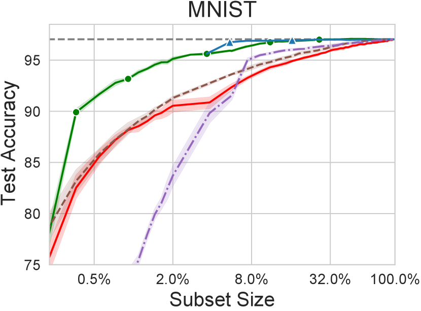
In the following experiment, we investigate coresets for multiclass logistic regression for MNIST and CIFAR-10. For MNIST, we use -dimensional Nyström features to approximate the feature map of the RBF kernel with . For CIFAR-10, we use the same setup as in Section 5.1. Figure 7 shows the comparison of one-by-one unweighted forward selection and weighted coreset generation via regularization (the algorithm is stopped when its test performance drops below the performance of the forward selection variant), to uniform sampling and -means in the feature space (we also compared to -center selection, which underperforms compared to -means), and to the two-stage selection of samples that are most frequently “forgotten” during training (misclassified at some point in training after being classified correctly before; referred to as “forgetting” in the figures) (Toneva et al., 2019)—we have also experimented with this method in the binary logistic regression experiment, but it significantly underperformed compared to uniform sampling under subset sizes of . Our proposed methods can achieve compression ratios of over (data set size divided by smallest data set size required for obtaining the same test accuracy) on both data sets with weighted coresets generated via regularization.

5.2.3 Neural Networks
For building small coresets () for neural networks, we find that construction via the Neural Tangent Kernel proxy is more effective—the experiments in the following sections concern such settings. For building large coresets, however, working with the original model is more effective. For computationally tractable implicit gradient evaluations for networks with millions of parameters, we evaluate unweighted coreset construction with batch forward selection and inverse Hessian-vector products approximated using the Neumann series (Lorraine et al., 2020). We truncate the series to terms and we introduce a scaling hyperparameter for the inner loss , such that the Neumann series approximation is now applied to . This is to ensure the converge of the Neumann series, for which a necessary and sufficient condition is , where denote the -th eigenvalue of (Chen, 2005). In automatic differentiation frameworks, Hessian-vector products can be calculated efficiently without instantiating the Hessian. However, due to memory considerations, we can only afford to evaluate on a single minibatch of data in the Hessian-vector products, which introduces another layer of approximation through the stochastic Hessian.


We demonstrate the effectiveness of bilevel coresets for wide residual networks (Zagoruyko and Komodakis, 2016) and search for the smallest coreset size such that the test performance matches the test performance of training on the full data set up to a tolerance. For computational considerations, we showcase the unweighted coreset construction via forward selection in batches of points, starting from a random pool of points. We evaluate the method by constructing coresets for a WideResNet-16-4 ( million parameters) on CIFAR-10 and SVHN (Netzer et al., 2011)—for SVHN we only use the train split, containing approximately images. We achieved the best results by retraining the network from scratch after every round of selection with SGD with momentum—further details about the training can be found in Appendix C.
We compare in Figure 8 our unweighted batch forward selection to the following subset selection methods for neural networks: uniform sampling, -means/-center in the pixel space (Nguyen et al., 2018), -means/-center in the last layer embedding of the trained network (Sener and Savarese, 2018), and selecting samples that are most frequently “forgotten” during training (Toneva et al., 2019). We plot each method’s test performance until they first reach the test performance of training on the full data set.
We find that, for both CIFAR-10 and SVHN, -means outperforms -center in the feature space, while -center is better for selection based on the last layer embeddings. The performance of -means/-center suggests that simple definitions of redundancy are suboptimal for constructing coresets. Figure 8 shows that our method achieves a compression ratio of on CIFAR-10 and on SVHN, i.e., it can find a representative subset of the training data of size () for CIFAR-10 and () for SVHN, such that the WideResNets trained on the chosen subsets achieve the test performance comparable to training on the full data set (within a margin of for CIFAR-10 and for SVHN). Whereas retaining points that are frequently forgotten (Toneva et al., 2019) matches the performance of our method for coreset sizes above () for CIFAR-10 and () for SVHN, it underperforms uniform sampling in generating small coresets.
An important application of data summarization is speeding up hyperparameter tuning, since the evaluations can be performed on the summary instead of the full data set. In neural architecture search, highly model-specific summaries are undesirable, as they might favor specific architectural choices. To inspect whether the coresets for WideResNet-16-4 are transferable to other architectures, we measure the performance of VGG16 (Simonyan and Zisserman, 2015) and MobileNetV2 (Sandler et al., 2018) adapted to CIFAR-10 and SVHN (kernel strides and pooling kernel sizes reduced to accommodate images) on coresets of size ; the training procedure is the same as for the WideResNet. Table 1 shows that, whereas the transferred coresets do not reach the full data set performance, they perform significantly better than uniform sampling and the transferred -center summary and perform similarly to the “forgetting” summary.
| CIFAR-10 | SVHN | |||
| VGG16 | MobileNetV2 | VGG16 | MobileNetV2 | |
| Uniform | ||||
| -center emb. | ||||
| Forgetting | ||||
| BiCo | ||||
| Full data set | ||||
We can improve the transferability of the coreset by building joint coresets for mulitple models, as proposed in Section 4.1. In the following experiment, we generate a joint coreset for WideResNet-16-4 and VGG16 and evaluate the resulting coreset for transferability on MobileNetV2. For this, we use a simple heuristic for approximating the solution of Equation (11) with : similarly to the previous experiment, we generate the coreset by forward greedy selection in batches of by alternating the model in each step (i.e., we select a new batch of points for the WideResNet, then for VGG16). The results in Table 2 show that this simple heuristic improves the effectiveness of the joint coreset on VGG16 and the transferability to MobileNetV2 at the expense of small performance degradation on WideResNet.
| data set | Architecture |
|
|
||||
|---|---|---|---|---|---|---|---|
| CIFAR-10 | WideResNet-16-4 | ||||||
| VGG16 | |||||||
| MobileNetV2 | |||||||
| SVHN | WideResNet-16-4 | ||||||
| VGG16 | |||||||
| MobileNetV2 |
5.3 Continual Learning
We compare our approach to existing replay memory management strategies by conducting an extensive experimental study. We focus continual learning setting where the learning algorithm is a neural network, and we keep the network structure fixed during learning on different tasks. This is known as the “single-head” setup, which is more challenging than instantiating new top layers for different tasks (“multi-head” setup) and does not assume any knowledge of the task descriptor during training and test time. For validating our coreset construction in the continual learning setting, we use the following -class classification data sets:
-
•
PMNIST (Goodfellow et al., 2014): consist of tasks, where in each task all images’ pixels undergo the same fixed random permutation.
-
•
SMNIST (Zenke et al., 2017): MNIST is split into tasks, where each task consists of distinguishing between consecutive image classes.
-
•
SCIFAR-10: similar to SMNIST on CIFAR-10.
Following Aljundi et al. (2019b), we keep a subsample of points for each task for all data sets while we retain the full test sets. For PMNIST, we use a fully connected net with two hidden layers with units, ReLU activations, and dropout with probability on the hidden layers. For SMNIST and SCIFAR-10, we use a CNN consisting of two blocks of convolution, dropout, max-pooling, and ReLU activation, where the number of filters are and and have size , followed by two fully connected layers of size and with dropout. The dropout probability is . We fix the replay memory size for tasks derived from MNIST. For SCIFAR-10, we the set the memory size to . We train our networks for epochs using Adam with step size after each task.
We perform an extensive comparison under the protocol described above of our method to other data selection methods proposed in the continual learning or the coreset literature—the detailed description of the baselines can be found in Appendix D. For each method, we report the test accuracy averaged over tasks on the best buffer regularization strength . For a fair comparison to other methods in terms of summary generation time, we restrict our coreset selection method in all of the continual learning experiments to forward selection of unweighted coresets via the Nyström proxy method with (Section 5.1)—we use the Neural Tangent Kernel (Jacot et al., 2018) corresponding to the chosen architecture, without dropout and max-pooling obtained with the library of Novak et al. (2020).
| Method | PMNIST | SMNIST | SCIFAR-10 |
|---|---|---|---|
| Training w/o replay | |||
| Uniform sampling | |||
| -means of features | |||
| -means of embeddings | |||
| -means of grads | |||
| -center of features | |||
| -center of embeddings | |||
| -center of grads | |||
| Gradient matching | |||
| Max entropy samples | |||
| Hardest samples | |||
| FRCL’s selection | |||
| iCaRL’s selection | |||
| BiCo |
We report the results in Table 3. We note that while several methods outperform uniform sampling on some data sets, only our method is consistently outperforming it on all data sets. For inspecting the gains obtained by our method over uniform sampling, we plot the final per-task test accuracy on SMNIST in Figure 9. We notice that our method’s advantage does not come from excelling at one task but rather by representing the majority of tasks better than uniform sampling. In Appendix D, we present a study of the effect of the replay memory size.
Our method can also be combined with different approaches to continual learning, such as variational continual learning (VCL) (Nguyen et al., 2018). Whereas VCL also relies on data summaries, it was proposed with uniform and -center summaries. We replace these with our coreset construction, and, following Nguyen et al. (2018), we conduct an experiment using a single-headed two-layer network with units per layer and ReLU activation, where the coreset size is set to points per task. The results in Table 4 corroborate the advantage of our method over simple selection rules and suggest that VCL can benefit from representative coresets.
| Method | PMNIST | SMNIST |
|---|---|---|
| -center | ||
| Uniform | ||
| BiCo |

5.4 Streaming
Streaming using neural networks has received little attention. To the best of our knowledge, the replay-based approach to streaming has been tackled by Aljundi et al. (2019b), who propose to select points in the replay memory that maximize the angles between pairs of gradients corresponding to the selected points, Hayes et al. (2019), who propose storing cluster centers per class and merging closest clusters for reduction, and Chrysakis and Moens (2020), who propose to class-balance reservoir sampling for imbalanced streams. We compare our method with these methods experimentally.
For evaluating our proposed coreset construction method for training neural networks in the streaming setting, we modify PMNIST and SMNIST by first concatenating all tasks for each data set and then streaming them in batches of size . We fix the replay memory size to and set the number of slots —the replay buffer is managed by the merge-reduce framework (Section 4.3). We train the models for gradient descent steps using Adam with step size after each batch. We use the same architectures as in the continual learning experiments.
| Method | PMNIST | SMNIST |
|---|---|---|
| Train on coreset | ||
| Reservoir | ||
| BiCo |
| Method | SMNIST | SCIFAR-10 |
|---|---|---|
| Reservoir | ||
| CBRS | ||
| BiCo |
We compare our coreset selection to reservoir sampling (Vitter, 1985) and the sample selection methods of Aljundi et al. (2019b) and Hayes et al. (2019). We were unable to tune the latter two to outperform reservoir sampling, except the gradient-based selection method of Aljundi et al. (2019b) on PMNIST, achieving a test accuracy of . Table 6 shows the dominance of our strategy over reservoir sampling. The table also shows the performance on training only once in the end of the stream on the created coreset, which alone provides strong performance, confirming the merge-reduce framework’s validity. We have also experimented with streaming on CIFAR-10 with buffer size , where our coreset construction did not outperform reservoir sampling. However, when the task representation in the stream is imbalanced, our method has significant advantages.
The setup of the streaming experiment favors reservoir sampling, as the data in the stream from different classes is balanced. We illustrate the benefit of our method in the more challenging scenario when the class representation is imbalanced. Similarly to Aljundi et al. (2019b), we create imbalanced streams from SMNIST and SCIFAR-10, by retaining random samples from the first four tasks and from the last task. In this setup, reservoir sampling will underrepresent the first tasks. For SMNIST we set the replay buffer size to while for SCIFAR-10 we use . We evaluate the test accuracy on the tasks individually, where we do not undersample the test set. We train the same CNN as in the continual learning experiments on the two imbalanced streams and set the number of slots to . We compare our method to reservoir sampling and class-balancing reservoir sampling (CBRS) (Chrysakis and Moens, 2020). The results in Table 6 confirm the flexibility of our framework and show that it is competitive with CBRS, which is specifically designed for imbalanced streams.
5.5 Batch Active Learning
We evaluate our proposed method focusing on the audio domain, where semi-supervised batch active learning has not yet been studied to the best of our knowledge. Our first contribution in this section is showing that semi-supervised strategies proposed in the image domain are also highly effective in audio keyword recognition tasks. Then, we show our batch selection strategy significantly outperforms other acquisition strategies on these tasks. Whereas our strategy is oblivious to the SSL algorithm, we choose MixMatch (Berthelot et al., 2019) as the semi-supervised learning algorithm due to its simplicity, ease of adaptation to the audio domain, and strong empirical performance.
For demonstrating the effectiveness of SSL and its combination with active learning in the audio domain, we focus on the Spoken Digit data set (Jackson, 2016) ( utterances, classes) and Speech Commands V2 (Warden, 2018) ( utterances, classes) data sets, both containing utterances of the length of one second or shorter. With the goal of applying deep neural network architectures from the image domain with minimal adaptations, we map the utterances to mel spectrograms by first resampling them to kHz and applying the mel feature extraction with of window length of ms, hop length of ms and bins.
We first investigate the advantages of data augmentation and semi-supervised learning. Our model is a Wide ResNet-28-10 (Zagoruyko and Komodakis, 2016) with weight decay of and without dropout, whereas the SSL algorithm is MixMatch with two augmentations for label guessing and unlabeled cost weight , with other hyperparameters are set to their defaults (Berthelot et al., 2019). As for data augmentation, we apply the following transformations in order with probability: i) amplitude change by , ii) audio speed change by , iii) random time shifts by ms, where , iv) mixing in background noise with SNR dB, where ; we use the noise segments from the Speech Commands data set.
| Spoken Digit Nr. of Labeled Samples | |||
|---|---|---|---|
| Method | |||
| Supervised w/o augm. | |||
| Supervised w augm. | |||
| MixMatch | |||
| Speech Commands Nr. of Labeled Samples | |||
| Supervised w/o augm. | |||
| Supervised w augm. | |||
| MixMatch | |||
We train the models with Adam with initial learning rate cosine annealed to over epochs. The results in Table 7 demonstrate the superiority of semi-supervised learning via MixMatch on the chosen keyword recognition tasks. These results are also strong indicators for the necessity of evaluating batch active learning in the semi-supervised setting. For this, we compare our proposed method with batch selection strategies compatible with semi-supervised learning. We note that some batch selection strategies not applicable with SSL: prominent examples are Bayesian techniques since the common semi-supervised losses do not have Bayesian interpretations. To this end, we implement uniform subsampling, max-entropy selection (predictions averaged over two augmentations), selection based on the -center algorithm in the last layer of the trained network (Sener and Savarese, 2018), the consistency-based batch selection of Gao et al. (2019) (with five augmentations for calculating the variance), and BADGE (Ash et al., 2020), that selects the batch based on the -means centers of the last layer gradient embeddings of the hard pseudo-labeled .
For our proposed method, we solve the coreset selection problem in Equation (12) with the CNTK proxy with cross-entropy loss (Section 5.1) with -dimensional features and we add penalty to the inner objective, turning it into strongly convex multiclass logistic regression problem. Furthermore, we use data augmentations for the inner problem: for each labeled point, we presample augmentations and concatenate them for batch gradient descent. We perform one-by-one forward selection, with approximate implicit gradients obtained using steps of conjugate gradients to generate the unweighted coreset.


| Nr. of Labeled Samples | ||||
| Spoken Digit | Speech Commands | |||
| Method | ||||
| Uniform | ||||
| Max-ent. | ||||
| k-center | ||||
| Consist. | - | - | ||
| BADGE | ||||
| BiCo | ||||

We compare the methods in the challenging setting of small labeled pools () and perform the acquisition in batches of size starting with and labeled samples for Spoken Digit and Speech Commands, respectively. The starting labeled pools are guaranteed to contain at least one sample from each class. We retrain the models from scratch in every active learning round.
The results in Figure 11 show a significant advantage of our method over other acquisition strategies with only a small number of labeled samples. Especially for Speech Commands, some acquisition strategies suffer from redundancy in the selected batch and, consequently, underperform compared to uniform sampling. We were unable to achieve good performance with the consistency-based acquisition (Gao et al., 2019) on Speech Commands—this phenomenon was also observed by the authors when starting the method with only a few labeled samples, who refer to it as “cold start failure”. We also evaluated starting the consistency-based acquisition after a larger number of labeled samples have been acquired by uniform sampling, but the method did not outperform uniform sampling.
We can gain insight into our proposed method by inspecting the chosen batches of points in the active learning round. For this, we plot the acquisitions in the first round of active learning on Spoken Digit data set in Figure 12, which represents points by their last layer embeddings (after training the network on the initial pool with test accuracy) mapped to two dimensions by t-SNE (van der Maaten and Hinton, 2011). The points chosen by our method represent a diverse batch where out of points are misclassified.
5.6 Dictionary Selection for Compressed Sensing
In this section, we showcase our framework for selecting dictionary measurement adaptively and incrementally on two examples in Figure 13: a synthetic data set containing a set of random sparse vectors, and the recovery of MNIST digits using a variational autoencoder as the generative model for the images. The baseline algorithms are randomly sampled measurements with normally distributed entries, which satisfy the RIP property with high probability, and approximate-greedy, which is inspired by the heuristics of Krause and Cevher (2010) to speed up the greedy algorithm by picking the measurements with the largest average inner product between the signal and the measurements. The classical greedy algorithm is too expensive given the dictionary sizes used here. The dictionary of linear measurements is chosen as a set of random matrices with entries distributed according to the unit normal distribution, or a wavelets basis for MNIST as done by Bora et al. (2017), which is a more challenging baseline since not necessarily all elements are equally sparse. In most cases, the compression ratio significantly improves when using our bilevel method.
5.7 Computational Cost
The time complexity of our algorithm depends on the variant and the model. We now discuss the case of batch forward selection for neural networks. The time complexity depends linearly i) on the number of outer iterations, which equals the coreset size divided by the forward step batch size ()—additionally, times the number of weight optimization rounds per step if weighting is used (); ii) the number of iterations for solving the inner problem in each step (); iii) the complexity of gradient calculations (); iv) the truncation in the Neumann series/the number of conjugate gradient iterations (); resulting in the total time complexity for unweighted bilevel coresets.
The proxy reformulation reduces the number of parameters to the order of the dimension of the Nyström features . On the other hand, the proxy reformulation introduces the overhead of calculating the proxy kernel, which might be a significant overhead for deep neural networks. We measure the time for generating coresets with the CNTK Nyström proxy with from a data set of points for the small CNN (SCNN) described in Section 5.3 and for the WideResNet-16-4 from Section 5.2. We calculate the corresponding NTKs without batch normalization and pooling with the library of Novak et al. (2020) on a single GeForce GTX Ti GPU, whereas the coreset selection is performed on a single CPU. The results are shown in Table 8.
Without the proxy reformulation, a single implicit gradient calculation (Equation 3) incurs the cost of calculating and and the cost of the Neumann series approximation. Each of these operations has to be performed in minibatches, requiring multiple backpropagation steps. We measure the cost of these operations for WideResNet-16-4 in Table 8, totaling to two minutes per implicit gradient calculation—for reference, we need implicit gradient calculations for generating the coreset of size for CIFAR-10 in Figure 8.
Another important consideration both in the proxy and the standard form is how to solve the inner optimization problem after an implicit gradient step. In all our applications except for deep neural networks Section 5.2, we resume the inner optimization after the gradient update with the optimal parameters found before the update and perform a small number of inner update steps. For deep neural networks trained with learning rate schedules, we find it beneficial to retrain our models from scratch after each forward batch selection step. A promising future direction is to speed up the selection process without a proxy for neural networks by eliminating the need for retraining from scratch.

| Op | SCNN | WideResNet-16-4 |
|---|---|---|
| NTK calc. | s | s |
| Coreset | s | s |
| Coreset | s | s |
| Op | Time |
|---|---|
| s | |
| Neumann s. | s |
| s |
6 Discussion and Conclusion
We presented a generic coreset construction framework applicable to any twice differentiable model without requiring model-specific adaptations. We proposed several variants for scaling up the basic algorithm to large coresets and large models. We showed that our method is effective for a wide range of models in various settings, outperforming specialized coreset constructions and other data summarization methods.
6.1 Limitations
We provide guarantees only for the case where the overall optimization objective is convex. Due to the hardness of the cardinality-constrained bilevel optimization problem, our method is only a heuristic for the non-convex settings. Except for the binary logistic regression experiments or kernelized linear regression, the cost of our proposed coreset construction is higher than the cost of training the model on the full data set. This contrasts with some of the previous coreset constructions’ goal to speed up the training process. Our method is thus suited for settings with memory or human resource constraints, as well as when the summary is reused (e.g., in hyperparameter tuning)—settings for which we demonstrated the effectiveness of our approach empirically in Section 5.
6.2 Future Work
The flexibility of our framework in accommodating different upper and lower level objectives allows for various extensions and applications. While we discussed some in this work, there are several promising directions, e.g., the framework could be extended to Bayesian inference by using objectives from variational inference. Furthermore, the idea of formulating subset selection as a cardinality-constrained bilevel optimization problem is very general and can be applied to problems besides coreset construction. Some notable examples include basis selection for the Nyström approximation, feature selection and neural network pruning.
Acknowledgments
This research was supported by the SNSF grant 407540_167212 through the NRP 75 Big Data program, by the European Research Council (ERC) under the European Union’s Horizon 2020 research, innovation programme grant agreement No 815943, and by the Swiss National Science Foundation through the NCCR Catalysis.
A Connection to Experimental Design
In this section, the weights are assumed to be binary, i.e., . We will use a shorthand for matrix where only rows of X whose indices are in are selected. This will be equivalent to selection done via the diagonal matrix , where corresponds to and zero otherwise. Additionally, let be a minimizer of the following loss,
| (14) |
which has the following closed form,
| (15) |
Frequentist Experimental Design.
Under the assumption that the data follows the linear model , where , we can show that the bilevel coreset framework instantiated with the inner objective (14) and , with various choices of outer objectives is related to frequentist optimal experimental design problems. The following propositions show how different outer objectives give rise to different experimental design objectives.
Proposition 4 (A-experimental design).
Under the linear regression assumptions and when , with the inner objective is equal to with , the objective simplifies,
Proof.
Using the closed form in (15), and model assumptions, we see that . Plugging this into the outer objective,
where in the third line we used the cyclic property of trace and subsequently the normality of . ∎
Proposition 5 (V-experimental design).
Under the linear regression assumptions and when and the inner objective is equal to with , the objective simplifies,
Proof.
Using the closed form in (15), and model assumptions, we see that . Plugging this in to the outer objective ,
where in the third line we used the cyclic property of trace and subsequently the normality of . ∎
Infinite data limit.
The following proposition links the data summarization objective and V-experimental design in the infinite data limit .
Proposition 6 (Infinite data limit).
Under the linear regression assumptions , , let be
the V-experimental design outer objective, and let the summarization objective be,
For all in Eq. (15), we have
Proof.
Since , we have,
We have since is a finite set. Since is independent of , ,
As a consequence, as .
∎
Note that Proposition 6 does not imply that our algorithm performs the same steps when used with instead of . It only means that the optimal solutions of the problems are converging to selections with the same quality in the infinite data limit.
Bayesian V-Experimental Design.
Bayesian experimental design (Chaloner and Verdinelli, 1995) can be incorporated as well into our framework. In Bayesian modeling, the “true” parameter is not a fixed value, but instead a sample from a prior distribution and hence a random variable. Consequently, upon taking into account the random nature of the coefficient vector, we can find an appropriate inner and outer objectives.
Proposition 7.
Under Bayesian linear regression assumptions and where , let the outer objective
where expectation is over the prior as well. Furthermore, let the inner objective be Eq. with the same value of , then the overall objective simplifies to
| (16) |
Proof.
Using the closed form in (15), and model assumptions, we see that . Plugging this in to the outer objective ,
where we used that , and cyclic property of the trace, and the final results follows by rearranging.
∎
Similarly to the case of unregularized frequentist experimental design, in the infinite data limit, even the Bayesian objectives share the same optima. The difference here is that the true parameter is no longer a fixed value and we need to integrate over it using the prior.
Proposition 8 (identical to Proposition 2).
Under the Bayesian linear regression assumptions , and , let be
the Bayesian V-experimental design outer objective, and let the summarization objective be,
For all in Eq. (15), we have
Proof.
The proof follows similarly as in Proposition 6. ∎
Lemma 9.
Assume for all and s.t. . The function
is convex and smooth in .
Proof.
We will show that the Hessian of is positive semi-definite (PSD) and that the maximum eigenvalue of the Hessian is bounded, which imply the convexity and smoothness of .
For brevity, we work with where . In addition, denote and s.t. . First, we would like to calculate , for which we will use directional derivatives:
To get , we should choose as direction where is on the -th position. Since , we have that:
We will proceed similarly to get .
Now, since,
we have
Choosing as our directional derivative, we have:
from which we can see that we can write the Hessian of in matrix form as:
where denotes the Hadamard product. Since is PSD it immediately follows that and are PSD. Since the Hadamard product of two PSD matrices is PSD due to the Schur product theorem, it follows that the Hessian is PSD and thus is convex.
As for smoothness, we need the largest eigenvalue of the Hessian to be bounded:
where in the fifth line we have used the property of the Rayleigh quotient that for any nonzero vector and self-adjoint matrix we have that . Thus is -smooth.
∎
B Connection to Influence Functions
Proof of Proposition 1
C Detailed Experimental Setup for Sections 5.1 and 5.2
Variants
All variants in Section 5.1 use regularizer in the inner problem. The inner optimization is performed with Adam using step size of as follows: all variants start with an optimization phase on the initial point set with iterations; then, after each step, an additional GD iterations are performed. We note that performing GD iterations on the entire data set takes seconds on a single GeForce GTX 1080 Ti.
Binary Logistic Regression
The features of the data sets are standardized to zero mean and unit variance. The logistic regression is solved using batch Adam with step size and -penalty of . For the bilevel coresets, the selection process is started from randomly chosen points and the implicit gradients are calculated through steps of conjugate gradients. For the unweighted version, gradient descent steps are performed after each selection. For the weighted version, we use Adam with step size to optimize the weights over outer iterations in each step.
We consider the following baselines:
-
•
-means in the feature space, where the chosen subset is the set of centers selected by -means++ (Arthur and Vassilvitskii, 2007); we also evaluated -center, which performed worse than -means on all data sets,
- •
-
•
Hilbert coresets (Campbell and Broderick, 2019) solved via Frank-Wolfe (Campbell and Broderick, 2019) and GIGA (Campbell and Broderick, 2018) with the norm chosen as the weighted Fisher information distance and with random features of dimensions. However, we were unable to tune either of these methods to outperform uniform sampling on any of the data sets, hence we do not show their performance.
Neural Networks
For training the networks, we use weight decay of and an initial learning rate of cosine-annealed to over epochs, where is the full data set size and is the subset size. Additionally, we use dropout with a rate of for SVHN. For CIFAR-10, we use the standard data augmentation pipeline of random cropping and horizontal flipping, whereas we do not use data augmentation for SVHN.
D Continual Learning and Streaming
For the continual learning experiments, we compare the following methods:
-
•
Training w/o replay: train after each task without replay memory. Demonstrates how catastrophic forgetting occurs.
-
•
Uniform sampling/per task coreset: the network is only trained on the points in the replay memory with different selection methods.
-
•
-means/-center in feature/embedding/gradient space: the per-task selection retains points in the replay memory that are generated by -means++ (Arthur and Vassilvitskii, 2007)/greedy -center algorithm, where the clustering is done either in the original feature space, in the last layer embedding of the neural network, or in the space of the gradient with respect to the last layer (after training on the respective task). The points that are the cluster centers in different spaces are the ones chosen to be saved in the memory. We note that the -center summarization in the last layer embedding space is the coreset method proposed for active learning by Sener and Savarese (2018).
- •
-
•
Training per task with FRCL’s/iCaRL’s selection: the points per task are selected by FRCL’s inducing point selection (Titsias et al., 2020), where the kernel is chosen as the linear kernel over the last layer embeddings/iCaRL’s selection (Algorithm 4 in Rebuffi et al. (2017)) performed in the normalized embedding space.
-
•
Gradient matching per task: same as iCaRL’s selection, but in the space of gradients with respect to the last layer and jointly over all classes. This is a variant of Hilbert coreset (Campbell and Broderick, 2019) with equal weights, where the Hilbert space norm is chosen to be the squared 2-norm difference of loss gradients with respect to the last layer at the maximum posterior value.
In the continual learning experiments, we train our networks for epochs using Adam with step size after each task. The loss at each step consists of the loss on a minibatch of size of the current tasks and loss on the replay memory scaled by . For streaming, we train our networks for gradient descent steps using Adam with step size after each batch. For Aljundi et al. (2019b), we use a streaming batch size of for better performance, as indicated in Section 2.4 of the supplementary materials of Aljundi et al. (2019b). We tune the replay memory regularization strength separately for each method from and report the best result on the test set.
| Method/Memory size | |||
|---|---|---|---|
| CL uniform sampling | |||
| CL BiCo | |||
| Streaming reservoir sampling | |||
| Streaming BiCo |
In our experiments, we used the Neural Tangent Kernel as proxy. It turns out that on the data sets derived from MNIST, simpler kernels such as RBF are also good proxy choices. To illustrate this, we repeat the continual learning and streaming experiments and report the results in Table 10. For the RBF kernel we set . While the RBF kernel is a good proxy for these data sets, it fails on harder data sets such as CIFAR-10.
| Method | PMNIST | SMNIST | |
|---|---|---|---|
| CL | BiCo CNTK | ||
| BiCo RBF | |||
| VCL | BiCo CNTK | ||
| BiCo RBF | |||
| Str. | BiCo CNTK | ||
| BiCo RBF |
References
- Agarwal et al. (2005) Pankaj K Agarwal, Sariel Har-Peled, Kasturi R Varadarajan, et al. Geometric approximation via coresets. Combinatorial and computational geometry, 52:1–30, 2005.
- Aljundi et al. (2019a) Rahaf Aljundi, Klaas Kelchtermans, and Tinne Tuytelaars. Task-free continual learning. In 2019 IEEE/CVF Conference on Computer Vision and Pattern Recognition (CVPR), pages 11254–11263. IEEE, June 2019a.
- Aljundi et al. (2019b) Rahaf Aljundi, Min Lin, Baptiste Goujaud, and Yoshua Bengio. Gradient based sample selection for online continual learning. In Advances in Neural Information Processing Systems (NeurIPS), pages 11816–11825. Curran Associates, Inc., 2019b.
- Arora et al. (2019) Sanjeev Arora, Simon S Du, Wei Hu, Zhiyuan Li, Russ R Salakhutdinov, and Ruosong Wang. On exact computation with an infinitely wide neural net. In Advances in Neural Information Processing Systems (NeurIPS), pages 8139–8148. Curran Associates, Inc., 2019.
- Arthur and Vassilvitskii (2007) David Arthur and Sergei Vassilvitskii. k-means++: The advantages of careful seeding. In Proceedings of the eighteenth annual ACM-SIAM symposium on Discrete algorithms, pages 1027–1035. Society for Industrial and Applied Mathematics, 2007.
- Ash et al. (2020) Jordan T. Ash, Chicheng Zhang, Akshay Krishnamurthy, John Langford, and Alekh Agarwal. Deep batch active learning by diverse, uncertain gradient lower bounds. In International Conference on Learning Representations (ICLR), 2020.
- Bach et al. (2012) Francis Bach, Rodolphe Jenatton, Julien Mairal, and Guillaume Obozinski. Optimization with sparsity-inducing penalties. Foundations and Trends in Machine Learning, 4(1):1–106, 2012.
- Bachem et al. (2017) Olivier Bachem, Mario Lucic, and Andreas Krause. Practical coreset constructions for machine learning. arXiv preprint arXiv:1703.06476, 2017.
- Badoiu and Clarkson (2003) Mihai Badoiu and Kenneth L. Clarkson. Smaller core-sets for balls. In Proceedings of the Fourteenth Annual ACM-SIAM Symposium on Discrete Algorithms, January 12-14, 2003, Baltimore, Maryland, USA, pages 801–802. ACM/SIAM, 2003.
- Balcan et al. (2007) Maria-Florina Balcan, Andrei Broder, and Tong Zhang. Margin based active learning. In International Conference on Computational Learning Theory (COLT), pages 35–50. Springer, 2007.
- Bandeira et al. (2013) Afonso S Bandeira, Edgar Dobriban, Dustin G Mixon, and William F Sawin. Certifying the restricted isometry property is hard. IEEE transactions on information theory, 59(6):3448–3450, 2013.
- Berthelot et al. (2019) David Berthelot, Nicholas Carlini, Ian Goodfellow, Nicolas Papernot, Avital Oliver, and Colin A Raffel. Mixmatch: A holistic approach to semi-supervised learning. In Advances in Neural Information Processing Systems (NeurIPS), pages 5049–5059, 2019.
- Bora et al. (2017) Ashish Bora, Ajil Jalal, Eric Price, and Alexandros G Dimakis. Compressed sensing using generative models. In International Conference on Machine Learning (ICLR), pages 537–546. PMLR, 2017.
- Borsos et al. (2020) Zalán Borsos, Mojmir Mutný, and Andreas Krause. Coresets via bilevel optimization for continual learning and streaming. In Advances in Neural Information Processing Systems (NeurIPS), volume 33, pages 14879–14890. Curran Associates, Inc., 2020.
- Borsos et al. (2021) Zalán Borsos, Marco Tagliasacchi, and Andreas Krause. Semi-supervised batch active learning via bilevel optimization. In ICASSP 2021-2021 IEEE International Conference on Acoustics, Speech and Signal Processing (ICASSP), pages 3495–3499. IEEE, 2021.
- Campbell and Broderick (2018) Trevor Campbell and Tamara Broderick. Bayesian coreset construction via greedy iterative geodesic ascent. In International Conference on Machine Learning, (ICML), pages 697–705. PMLR, 2018.
- Campbell and Broderick (2019) Trevor Campbell and Tamara Broderick. Automated scalable bayesian inference via hilbert coresets. The Journal of Machine Learning Research, 20(1):551–588, 2019.
- Candes et al. (2006) Emmanuel J Candes, Justin K Romberg, and Terence Tao. Stable signal recovery from incomplete and inaccurate measurements. Communications on Pure and Applied Mathematics: A Journal Issued by the Courant Institute of Mathematical Sciences, 59(8):1207–1223, 2006.
- Chaloner and Verdinelli (1995) Kathryn Chaloner and Isabella Verdinelli. Bayesian experimental design: A review. Statist. Sci., 10(3):273–304, August 1995. ISSN 0883-4237.
- Chaudhry et al. (2019) Arslan Chaudhry, Marcus Rohrbach, Mohamed Elhoseiny, Thalaiyasingam Ajanthan, Puneet K Dokania, Philip HS Torr, and Marc’Aurelio Ranzato. Continual learning with tiny episodic memories. arXiv preprint arXiv:1902.10486, 2019.
- Chazelle and Matoušek (1996) Bernard Chazelle and Jiři Matoušek. On linear-time deterministic algorithms for optimization problems in fixed dimension. J. Algorithm., 21(3):579–597, November 1996. ISSN 0196-6774.
- Chen (2005) Ke Chen. Matrix Preconditioning Techniques and Applications. Cambridge Monographs on Applied and Computational Mathematics. Cambridge University Press, July 2005.
- Chrysakis and Moens (2020) Aristotelis Chrysakis and Marie-Francine Moens. Online continual learning from imbalanced data. In International Conference on Machine Learning (ICML), pages 1952–1961. PMLR, 2020.
- Clarkson (2010) Kenneth L. Clarkson. Coresets, sparse greedy approximation, and the frank-wolfe algorithm. ACM Trans. Algorithms, 6(4):63:1–63:30, 2010.
- Coleman et al. (2020) Cody Coleman, Christopher Yeh, Stephen Mussmann, Baharan Mirzasoleiman, Peter Bailis, Percy Liang, Jure Leskovec, and Matei Zaharia. Selection via proxy: Efficient data selection for deep learning. In International Conference on Learning Representations (ICLR), 2020.
- Cook and Weisberg (1980) R. Dennis Cook and Sanford Weisberg. Characterizations of an empirical influence function for detecting influential cases in regression. Technometrics, 22(4):495–508, November 1980. ISSN 0040-1706, 1537-2723.
- Cook and Weisberg (1982) R Dennis Cook and Sanford Weisberg. Residuals and influence in regression. New York: Chapman and Hall, 1982.
- Donoho (2006) David L Donoho. Compressed sensing. IEEE Transactions on information theory, 52(4):1289–1306, 2006.
- Dua and Graff (2017) Dheeru Dua and Casey Graff. UCI machine learning repository, 2017. URL http://archive.ics.uci.edu/ml.
- Duchi et al. (2008) John Duchi, Shai Shalev-Shwartz, Yoram Singer, and Tushar Chandra. Efficient projections onto thel1-ball for learning in high dimensions. In International Conference on Machine learning (ICML), pages 272–279, 2008.
- Fanello et al. (2013) Sean Ryan Fanello, Carlo Ciliberto, Matteo Santoro, Lorenzo Natale, Giorgio Metta, Lorenzo Rosasco, and Francesca Odone. icub world: Friendly robots help building good vision data-sets. In 2013 IEEE Conference on Computer Vision and Pattern Recognition Workshops, pages 700–705. IEEE, June 2013. ISBN 9780769549903.
- Fedorov (1972) Valerii V. Fedorov. Theory of optimal experiments. Probability and mathematical statistics. Academic Press, New York, NY, USA, 1972.
- Feldman (2020) Dan Feldman. Introduction to core-sets: an updated survey. arXiv preprint arXiv:2011.09384, 2020.
- Feldman and Langberg (2011) Dan Feldman and Michael Langberg. A unified framework for approximating and clustering data. In Proceedings of the 43rd annual ACM symposium on Theory of computing - STOC ’11, pages 569–578. ACM, ACM Press, 2011.
- Finn et al. (2017) Chelsea Finn, Pieter Abbeel, and Sergey Levine. Model-agnostic meta-learning for fast adaptation of deep networks. In International Conference on Machine Learning (ICML), pages 1126–1135, 2017.
- Franceschi et al. (2017) Luca Franceschi, Michele Donini, Paolo Frasconi, and Massimiliano Pontil. Forward and reverse gradient-based hyperparameter optimization. In International Conference on Machine Learning (ICML), pages 1165–1173. PMLR, 2017.
- Franceschi et al. (2018) Luca Franceschi, Paolo Frasconi, Saverio Salzo, Riccardo Grazzi, and Massimiliano Pontil. Bilevel programming for hyperparameter optimization and meta-learning. In International Conference on Machine Learning (ICML), pages 1568–1577. PMLR, 2018.
- Frank and Wolfe (1956) Marguerite Frank and Philip Wolfe. An algorithm for quadratic programming. Nav. Res. Log., 3(1-2):95–110, March 1956. ISSN 0028-1441, 1931-9193.
- French (1999) R French. Catastrophic forgetting in connectionist networks. Trends Cogn. Sci., 3(4):128–135, April 1999. ISSN 1364-6613.
- Gao et al. (2019) Mingfei Gao, Zizhao Zhang, Guo Yu, Sercan O Arik, Larry S Davis, and Tomas Pfister. Consistency-based semi-supervised active learning: Towards minimizing labeling cost. arXiv preprint arXiv:1910.07153, 2019.
- Goodfellow et al. (2014) Ian J. Goodfellow, Mehdi Mirza, Da Xiao, Aaron Courville, and Yoshua Bengio. An empirical investigation of catastrophic forgetting in gradient-based neural networks. In International Conference on Learning Representations (ICLR), 2014.
- Guo and Schuurmans (2008) Yuhong Guo and Dale Schuurmans. Discriminative batch mode active learning. In Advances in neural information processing systems, pages 593–600, 2008.
- Har-peled (2011) Sariel Har-peled. Geometric Approximation Algorithms. American Mathematical Society, USA, 2011. ISBN 0821849115.
- Har-Peled and Mazumdar (2004) Sariel Har-Peled and Soham Mazumdar. On coresets for k-means and k-median clustering. In Proceedings of the thirty-sixth annual ACM symposium on Theory of computing - STOC ’04, pages 291–300. ACM, ACM Press, 2004. ISBN 1581138520.
- Hayes et al. (2019) Tyler L. Hayes, Nathan D. Cahill, and Christopher Kanan. Memory efficient experience replay for streaming learning. In 2019 International Conference on Robotics and Automation (ICRA). IEEE, IEEE, May 2019. ISBN 9781538660270.
- Hoi and Lyu (2005) Steven C.H. Hoi and M.R. Lyu. A semi-supervised active learning framework for image retrieval. In 2005 IEEE Computer Society Conference on Computer Vision and Pattern Recognition (CVPR), pages 302–309 vol. 2. IEEE, 2005.
- Hoi et al. (2006) Steven C.H. Hoi, Rong Jin, Jianke Zhu, and Michael R. Lyu. Batch mode active learning and its application to medical image classification. In International Conference on Machine learning (ICML), pages 417–424. ACM Press, 2006.
- Huggins et al. (2016) Jonathan Huggins, Trevor Campbell, and Tamara Broderick. Coresets for scalable bayesian logistic regression. In Advances in Neural Information Processing Systems (NeurIPS), pages 4080–4088, 2016.
- Jackson (2016) Zohar Jackson. Free spoken digit dataset, 2016. https://github.com/Jakobovski/free-spoken-digit-dataset.
- Jacot et al. (2018) Arthur Jacot, Franck Gabriel, and Clément Hongler. Neural tangent kernel: Convergence and generalization in neural networks. In Advances in neural information processing systems (NeurIPS), pages 8571–8580, 2018.
- Jalal et al. (2021) Ajil Jalal, Sushrut Karmalkar, Alexandros G Dimakis, and Eric Price. Instance-optimal compressed sensing via posterior sampling. In International Conference on Machine Learning (ICML). PMLR, 2021.
- Killamsetty et al. (2021) Krishnateja Killamsetty, Durga Sivasubramanian, Ganesh Ramakrishnan, and Rishabh Iyer. Glister: Generalization based data subset selection for efficient and robust learning. AAAI Conference on Artificial Intelligence, 35(9):8110–8118, May 2021.
- Kirkpatrick et al. (2017) James Kirkpatrick, Razvan Pascanu, Neil Rabinowitz, Joel Veness, Guillaume Desjardins, Andrei A. Rusu, Kieran Milan, John Quan, Tiago Ramalho, Agnieszka Grabska-Barwinska, Demis Hassabis, Claudia Clopath, Dharshan Kumaran, and Raia Hadsell. Overcoming catastrophic forgetting in neural networks. Proc Natl Acad Sci USA, 114(13):3521–3526, March 2017. ISSN 0027-8424, 1091-6490.
- Kirsch et al. (2019) Andreas Kirsch, Joost van Amersfoort, and Yarin Gal. Batchbald: Efficient and diverse batch acquisition for deep bayesian active learning. In Advances in Neural Information Processing Systems (NeurIPS), pages 7026–7037, 2019.
- Koh and Liang (2017) Pang Wei Koh and Percy Liang. Understanding black-box predictions via influence functions. In International Conference on Machine Learning (ICML), pages 1885–1894. JMLR. org, 2017.
- Krause and Cevher (2010) Andreas Krause and Volkan Cevher. Submodular dictionary selection for sparse representation. In International Conference on Machine Learning (ICML), pages 567–574, June 2010.
- Langberg and Schulman (2010) Michael Langberg and Leonard J. Schulman. Universal -approximators for integrals. In Proceedings of the Twenty-First Annual ACM-SIAM Symposium on Discrete Algorithms, pages 598–607. SIAM, Society for Industrial and Applied Mathematics, January 2010. ISBN 9780898717013.
- Leng et al. (2013) Yan Leng, Xinyan Xu, and Guanghui Qi. Combining active learning and semi-supervised learning to construct svm classifier. Knowl-based. Syst., 44:121–131, May 2013. ISSN 0950-7051.
- Lewis and Gale (1994) David D Lewis and William A Gale. A sequential algorithm for training text classifiers. In SIGIR’94, pages 3–12. Springer, 1994.
- Li et al. (2017) Zhenguo Li, Fengwei Zhou, Fei Chen, and Hang Li. Meta-sgd: Learning to learn quickly for few-shot learning. arXiv preprint arXiv:1707.09835, 2017.
- Liu et al. (2019) Hanxiao Liu, Karen Simonyan, and Yiming Yang. DARTS: Differentiable architecture search. In International Conference on Learning Representations (ICLR), 2019.
- Locatello et al. (2017) Francesco Locatello, Michael Tschannen, Gunnar Rätsch, and Martin Jaggi. Greedy algorithms for cone constrained optimization with convergence guarantees. In Advances in Neural Information Processing Systems (NeurIPS), pages 773–784, 2017.
- Lopez-Paz and Ranzato (2017) David Lopez-Paz and Marc’Aurelio Ranzato. Gradient episodic memory for continual learning. In Advances in Neural Information Processing Systems (NeurIPS), pages 6467–6476, 2017.
- Lorraine et al. (2020) Jonathan Lorraine, Paul Vicol, and David Duvenaud. Optimizing millions of hyperparameters by implicit differentiation. In International Conference on Artificial Intelligence and Statistics (AISTATS), pages 1540–1552. PMLR, 2020.
- Lucic et al. (2017) Mario Lucic, Matthew Faulkner, Andreas Krause, and Dan Feldman. Training gaussian mixture models at scale via coresets. The Journal of Machine Learning Research, 18(1):5885–5909, 2017.
- MacKay (1992) David J.C. MacKay. Information-based objective functions for active data selection. Neural Comput., 4(4):590–604, July 1992. ISSN 0899-7667, 1530-888X.
- Mahoney and Drineas (2009) Michael W. Mahoney and Petros Drineas. Cur matrix decompositions for improved data analysis. PNAS, 106(3):697–702, January 2009. ISSN 0027-8424, 1091-6490.
- McCloskey and Cohen (1989) Michael McCloskey and Neal J. Cohen. Catastrophic interference in connectionist networks: The sequential learning problem. In Psychology of Learning and Motivation, volume 24, pages 109–165. Elsevier, 1989. ISBN 9780125433242.
- Mirzasoleiman et al. (2020) Baharan Mirzasoleiman, Jeff Bilmes, and Jure Leskovec. Coresets for data-efficient training of machine learning models. In International Conference on Machine Learning (ICML), pages 6950–6960. PMLR, 2020.
- Mitchell (1974) Toby J. Mitchell. An algorithm for the construction of "d-optimal" experimental designs. Technometrics, 16(2):203, May 1974. ISSN 0040-1706.
- Netzer et al. (2011) Yuval Netzer, Tao Wang, Adam Coates, Alessandro Bissacco, Bo Wu, and Andrew Y Ng. Reading digits in natural images with unsupervised feature learning. NIPS Workshop on Deep Learning and Unsupervised Feature Learning 2011, 2011.
- Nguyen et al. (2018) Cuong V. Nguyen, Yingzhen Li, Thang D. Bui, and Richard E. Turner. Variational continual learning. In International Conference on Learning Representations (ICLR), 2018.
- Novak et al. (2020) Roman Novak, Lechao Xiao, Jiri Hron, Jaehoon Lee, Alexander A. Alemi, Jascha Sohl-Dickstein, and Samuel S. Schoenholz. Neural tangents: Fast and easy infinite neural networks in python. In International Conference on Learning Representations (ICLR), 2020.
- Pedregosa (2016) Fabian Pedregosa. Hyperparameter optimization with approximate gradient. In International Conference on Machine Learning (ICML), pages 737–746, 2016.
- Phillips (2016) Jeff M. Phillips. Coresets and sketches. arXiv preprint arXiv:1601.00617, 2016.
- Rebuffi et al. (2017) Sylvestre-Alvise Rebuffi, Alexander Kolesnikov, Georg Sperl, and Christoph H. Lampert. icarl: Incremental classifier and representation learning. In IEEE Conference on Computer Vision and Pattern Recognition (CVPR), pages 2001–2010. IEEE, 2017.
- Rusu et al. (2016) Andrei A Rusu, Neil C Rabinowitz, Guillaume Desjardins, Hubert Soyer, James Kirkpatrick, Koray Kavukcuoglu, Razvan Pascanu, and Raia Hadsell. Progressive neural networks. arXiv preprint arXiv:1606.04671, 2016.
- Sandler et al. (2018) Mark Sandler, Andrew Howard, Menglong Zhu, Andrey Zhmoginov, and Liang-Chieh Chen. Mobilenetv2: Inverted residuals and linear bottlenecks. In IEEE/CVF Conference on Computer Vision and Pattern Recognition, pages 4510–4520. IEEE, 2018.
- Sener and Savarese (2018) Ozan Sener and Silvio Savarese. Active learning for convolutional neural networks: A core-set approach. In International Conference on Learning Representations (ICLR), 2018.
- Shin et al. (2017) Hanul Shin, Jung Kwon Lee, Jaehong Kim, and Jiwon Kim. Continual learning with deep generative replay. In Advances in Neural Information Processing Systems (NeurIPS), pages 2990–2999, 2017.
- Simonyan and Zisserman (2015) Karen Simonyan and Andrew Zisserman. Very deep convolutional networks for large-scale image recognition. In International Conference on Learning Representations, 2015.
- Sohn et al. (2020) Kihyuk Sohn, David Berthelot, Nicholas Carlini, Zizhao Zhang, Han Zhang, Colin A Raffel, Ekin Dogus Cubuk, Alexey Kurakin, and Chun-Liang Li. Fixmatch: Simplifying semi-supervised learning with consistency and confidence. In Advances in Neural Information Processing Systems (NeurIPS), pages 596–608. Curran Associates, Inc., 2020.
- Song et al. (2019) Shuang Song, David Berthelot, and Afshin Rostamizadeh. Combining mixmatch and active learning for better accuracy with fewer labels. arXiv preprint arXiv:1912.00594, 2019.
- Tapia et al. (2020) Javier Tapia, Espen Knoop, Mojmir Mutný, Miguel A. Otaduy, and Moritz Bächer. Makesense: Automated sensor design for proprioceptive soft robots. Soft Rob., 7(3):332–345, June 2020. ISSN 2169-5172, 2169-5180.
- Tarvainen and Valpola (2017) Antti Tarvainen and Harri Valpola. Mean teachers are better role models: Weight-averaged consistency targets improve semi-supervised deep learning results. In Advances in Neural Information Processing Systems (NeurIPS. Curran Associates, Inc., 2017.
- Tibshirani (1996) Robert Tibshirani. Regression shrinkage and selection via the lasso. Journal of the Royal Statistical Society: Series B (Methodological), 58(1):267–288, January 1996. ISSN 0035-9246.
- Titsias et al. (2020) Michalis K. Titsias, Jonathan Schwarz, Alexander G. de G. Matthews, Razvan Pascanu, and Yee Whye Teh. Functional regularisation for continual learning with gaussian processes. In International Conference on Learning Representations (ICLR), 2020.
- Toneva et al. (2019) Mariya Toneva, Alessandro Sordoni, Remi Tachet des Combes, Adam Trischler, Yoshua Bengio, and Geoffrey J. Gordon. An empirical study of example forgetting during deep neural network learning. In International Conference on Learning Representations (ICLR), 2019.
- Tsang et al. (2005) Ivor W. Tsang, James T. Kwok, and Pak-Ming Cheung. Core vector machines: Fast svm training on very large data sets. Journal of Machine Learning Research, 6(13):363–392, 2005.
- Uzilov et al. (2006) Andrew V Uzilov, Joshua M Keegan, and David H Mathews. Detection of non-coding rnas on the basis of predicted secondary structure formation free energy change. BMC Bioinf., 7(1):173, 2006. ISSN 1471-2105.
- van der Maaten and Hinton (2011) Laurens van der Maaten and Geoffrey Hinton. Visualizing non-metric similarities in multiple maps. Mach Learn, 87(1):33–55, December 2011. ISSN 0885-6125, 1573-0565.
- Vicente et al. (1994) L. Vicente, G. Savard, and J. Júdice. Descent approaches for quadratic bilevel programming. J Optim Theory Appl, 81(2):379–399, May 1994. ISSN 0022-3239, 1573-2878.
- Vicente and Calamai (1994) Luis N. Vicente and Paul H. Calamai. Bilevel and multilevel programming: A bibliography review. J Glob Optim, 5(3):291–306, October 1994. ISSN 0925-5001, 1573-2916.
- Vitter (1985) Jeffrey S. Vitter. Random sampling with a reservoir. ACM Trans. Math. Softw., 11(1):37–57, March 1985. ISSN 0098-3500, 1557-7295.
- von Stackelberg and Peacock (1952) H. von Stackelberg and A. Peacock. The Theory of the market economy. Hodge, 1952.
- Wang et al. (2018) Tianyang Wang, Jun Huan, and Bo Li. Data dropout: Optimizing training data for convolutional neural networks. In 2018 IEEE 30th International Conference on Tools with Artificial Intelligence (ICTAI), pages 39–46. IEEE, IEEE, November 2018. ISBN 9781538674499.
- Warden (2018) P. Warden. Speech Commands: A Dataset for Limited-Vocabulary Speech Recognition. arXiv preprint arXiv:1804.03209, 2018.
- Wei et al. (2015) Kai Wei, Rishabh Iyer, and Jeff Bilmes. Submodularity in data subset selection and active learning. In Francis Bach and David Blei, editors, International Conference on Machine Learning (ICML), pages 1954–1963. PMLR, 2015.
- Williams and Seeger (2001) Christopher Williams and Matthias Seeger. Using the nyström method to speed up kernel machines. In Advances in Neural Information Processing Systems (NeurIPS), pages 682–688. MIT Press, 2001.
- Wu et al. (2018) Yuhuai Wu, Mengye Ren, Renjie Liao, and Roger Grosse. Understanding short-horizon bias in stochastic meta-optimization. In International Conference on Learning Representations, 2018.
- Zagoruyko and Komodakis (2016) Sergey Zagoruyko and Nikos Komodakis. Wide residual networks. arXiv preprint arXiv:1605.07146, 2016.
- Zenke et al. (2017) Friedemann Zenke, Ben Poole, and Surya Ganguli. Continual learning through synaptic intelligence. In International Conference on Machine Learning (ICML), pages 3987–3995. PMLR, 2017.
- Zhao et al. (2021) Bo Zhao, Konda Reddy Mopuri, and Hakan Bilen. Dataset condensation with gradient matching. In International Conference on Learning Representations (ICLR), 2021.
- Zhu et al. (2003) Xiaojin Zhu, Zoubin Ghahramani, and John D. Lafferty. Semi-supervised learning using gaussian fields and harmonic functions. In International Conference (ICML), pages 912–919, 2003.