Data Processing Techniques for Ion and Electron Energy Distribution Functions
Abstract
Retarding field energy analyzers and Langmuir probes are routinely used to obtain ion and electron energy distribution functions (IEDF, EEDF). These typically require knowledge of the first and second derivatives of the - characteristics, both of which can be obtained in various ways. This poses challenges inherent to differentiating noisy signals, a frequent problem with electric-probe plasma diagnostics. A brief review of commonly used analog and numerical filtering and differentiation techniques is presented, together with their application on experimental data collected in a radio-frequency plasma. The application of each method is detailed with regards to the obtained IEDF and EEDF, the deduced plasma parameters, dynamic range, energy resolution and signal distortion.
I Introduction
Distribution functions offer a detailed description of plasma charged particles: from obtaining some useful plasma parameters (e.g. density, temperature and potential) to deducing heating and transport mechanisms, collision and reaction rates, as well as detecting the presence of particles sub-populations Godyak, Piejak, and Alexandrovich (1993); Charles and Boswell (2004); Takahashi et al. (2009); Boswell et al. (2015). The ion-energy distribution function (IEDF) is extensively employed to characterize the ion kinetics in plasma processing techniques and in the development of spacecraft electric propulsion technologies, where the detection of accelerated ion populations, such as ion beams, is important Charles and Boswell (2004); Ingram and Braithwaite (1988); Habl, Rafalskyi, and Lafleur (2020). The electron-energy distribution function (EEDF) gives an extensive picture of the dynamics of electrons. This is essential for characterizing the plasma generation mechanisms in laboratory and commercial plasma devices, as well as in investigating fundamental aspects of plasma physics, e.g. the thermodynamics of magnetized electrons Godyak, Piejak, and Alexandrovich (1992a); Takahashi et al. (2020).
Electrostatic probes, such as retarding field energy analyzers (RFEA) and single Langmuir probes (LP), are some of the most common instruments for measuring ion and electron distribution functions, respectively. The plasma potential, and the ion beam potential and density are usually obtained through the first derivative of an RFEA - characteristic. From a Langmuir probe - characteristic, the floating potential, electron temperature, plasma density, and plasma potential can be inferred via the classical Langmuir method Mott-Smith and Langmuir (1926); Merlino (2007). While popular thanks to its apparent simplicity, this method is only valid for plasmas with Maxwellian electron distributions and can be inaccurate in determining the plasma potential and ion current Godyak and Demidov (2011); Godyak (2021). Alternatively, the Druyvesteyn method directly determines the electron distribution function from the second derivative of the LP - characteristics, a process inherently more robust and information-rich than the Langmuir method, yet more challenging owing to the double differentiation Druyvesteyn (1930).
The ion-energy distribution function has usually been computed by obtaining the first derivative of the collected current over the discriminator voltage Böhm and Perrin (1993); Charles et al. (2000); Charles and Boswell (2004); Cox et al. (2008); Takahashi, Shida, and Fujiwara (2010); Bennet, Charles, and Boswell (2018); Ingram and Braithwaite (1988); Habl, Rafalskyi, and Lafleur (2020); Imai and Takahashi (2022). It can be shown that, by assuming a one-dimensional velocity distribution Böhm and Perrin (1993), the ion-energy distribution is proportional to the negative derivative of the collected current with respect to the discriminator grid voltage :
| (1) |
where is the probe grid transmission factor (four grids in the case of the RFEA used in this work) Charles and Boswell (2004), is the area of the probe orifice, and is the ion mass. Thus, the IEDF can be calculated simply by differentiating the measured current with respect to the discriminator voltage. For a single Gaussian distribution, the voltage at which the IEDF peak occurs is defined as the local plasma potential, . If a population of accelerating ions is present, as in the case of a plasma expanding through a double-layer Charles and Boswell (2004); Keesee et al. (2005); Bennet, Charles, and Boswell (2018) and for the considered gas pressures (i.e., 0.2 - 1 mTorr), the IEDF would show a second peak at a higher energy located at the ion beam potential, .
Druyvesteyn (1930) showed that for an isotropic plasma, the EEDF is proportional to the second derivative of the electron current from the - characteristic of a Langmuir probe. The relationship between the EEDF and the second derivative of the LP electron current with respect to the biasing voltage is
| (2) |
Here, and is the local plasma potential. is the electron energy in electronvolts, is the probe area, is the elementary charge and the electron mass. The electron probability distribution function (EEPF) is then . In an isotropic electron gas, the EEDF and EEPF contain the same information as the electron distribution function (which includes the velocity space). The local plasma potential is found from the zero crossing of . The the electron density can be retrieved from
| (3) |
and the effective electron temperature can be calculated from the average electron energy as
| (4) |
Plotting the natural logarithm of the EEPF can show a departure from a Maxwellian energy distribution function if the slope of the EEPF is not linear, e.g. bi-Maxwellian or Druyvesteynian. If the EEPF is Maxwellian, the electron temperature can also be deduced from the slope of the natural logarithm of the EEPF and is equal to .
IEDF and EEDF are usually obtained through a variety of analog and numerical differentiation routines. Since measurement noise amplification is inherent to the differentiation process, filtering/fitting methods may be necessary to smooth the measured - data without causing significant distortion and to obtain accurate first and second derivatives. Among the numerical methods, the Savitzky-Golay filter is one of the most commonly employed for IEDF/EEDF derivations Savitzky and Golay (1964); Sudit and Woods (1993); Bétchu et al. (2013); Conde et al. (2017); Damba et al. (2018). Fernández Palop et al. (1995) implemented a Gaussian filter to smooth the - characteristics and evaluate the electron-energy distribution function. This method was compared with the Savitzky-Golay filter and the B-spline approximation methods. Magnus and Gudmundsson (2008) compared the use of the Savitzky-Golay filter, as well as the Gaussian filter, the Blackman window and polynomial fitting, to smooth both simulated and experimental - curves. The mean squared error, the correlation coefficient and the residuals of the different methods were compared, coupled with a visual assessment of the EEPF. Alternatively, analog differentiation has been performed by using appropriate electronics circuitry to obtain the IEDF and the EEPF Sloane and MacGregor (1934); Godyak, Piejak, and Alexandrovich (1992b); Takahashi et al. (2009); Takahashi, Shida, and Fujiwara (2010); Yadav et al. (2018). The IEDF has also been obtained using a Gaussian deconvolution method Charles and Boswell (2004); Cox et al. (2008); Imai and Takahashi (2022).
The aim of this paper is to review different signal processing and differentiation methods for the acquisition of optimal ion- and electron-energy distribution functions. The study discusses analog and numerical processing techniques that are routinely used to obtain EEDFs and IEDFs. With respect to the latter, the focus is on processing IEDFs that show the presence of multiple ion populations. The different numerical processes reviewed to obtain the first and second derivatives from the I-V characteristics are: Savitzky-Golay (SG) filter, B-spline piecewise polynomial fitting (BS), Gaussian filter (GF), and the Blackman window filter (BW). The ion-energy distribution function is also computed using the Gaussian deconvolution method. The analysis presented is intended as a baseline approach for the manipulation of - characteristics obtained from experimental data in a plasma discharge. Specifically, data collected in a magnetized radio-frequency plasma discharge at low gas pressures are used, which contain a higher noise level than, e.g. DC plasma discharges. This work gathers the lessons learned in the acquisition and processing of electric probe data to ease the reader’s process of obtaining charged-particles energy distribution functions of suitable quality.
The work is organized as follows; Section II describes the experimental set-up, including the plasma diagnostic probes. Section III introduces the analog and numerical filtering/differentiation methods employed. Finally, Section IV provides an example application of data processing analysis for ion- and electron-energy distribution functions obtained from the different methods starting from raw experimental data.
II Apparatus & Diagnostics
II.1 Apparatus
The data used in this study has been acquired using Moa Caldarelli et al. (2022), a radio-frequency plasma reactor that is an expansion of Huia Filleul et al. (2021, 2022). It consists of a cm long, cm inner diameter borosilicate glass tube plasma source connected to a cm long, cm diameter steel expansion chamber hosting the pumping system and the pressure gauges. The location of the interface between the plasma source and the expansion chamber is defined as cm. A base pressure of Torr is routinely achieved, while the argon working pressure ranges between Torr and Torr. The plasma is triggered and energized in the plasma source using a - turns loop antenna connected through an L-type matching network to a kW RF generator working at MHz. A static magnetic field is applied with a pair of movable Helmholtz solenoids, placed concentrically with the glass tube. The coils position along the plasma source length can be adjusted to obtain the desired magnetic field topology.
II.2 Retarding Field Energy Analyzer
The retarding field energy analyzer used to measure the ion-energy distribution function consists of four mesh grids (namely, earth, repeller, discriminator, and secondary grid) and a nickel collector plate that collects the incoming ion flux. The grids are made of a nickel mesh with a transmission factor of 59% which are attached to a copper support. The probe orifice has a diameter of mm, and a mm thick polyimide sheet is used to electrically insulate the grids and the collector plate. The design of this probe has been extensively used in similar experiments Charles et al. (2000); Charles and Boswell (2004); Cox et al. (2010); Bennet, Charles, and Boswell (2018), and a detailed description of the RFEA and its electric circuit used herein are presented in Ref. Caldarelli et al., 2021. In order to map the energy of the ions, the voltage of the discriminator grid is swept from V to V to obtain the - characteristics. It has to be noted that from RFEA measurements, only the energy distribution function of the ions that fall through the probe sheath within an acceptance angle of are obtained Charles and Boswell (2004). When taking measurements of the ion current in an RF plasma with an RFEA, the collected data can be affected by different mechanisms. In particular, in an RF excited plasma, broadening of the energy distribution caused by RF modulation can be observed Conway, Perry, and Boswell (1998); Charles et al. (2000); Charles and Boswell (2004) that could lead to peak separation, giving false data on the presence of different ion populations. Additionally, possible ion-neutral collisions (elastic and charge-exchange) occurring in the probe sheath and inside the analyzer could also affect the collected ion energy. However, for the low-pressure case analyzed, collisions inside the RFEA and in the sheath can be considered negligible, i.e. (where is the sheath width in front of the RFEA and is the repeller-discriminator grid distance).
II.3 RF Compensated Langmuir Probe
As from Langmuir’s work, sizing a single Langmuir probe requires the plasma volume disturbed by the probe to be much smaller than the electron mean free path Godyak and Demidov (2011). This ensures that the probe only disturbs the plasma in ways that can be accounted for by theory. Following recommendations in Ref. Godyak, 2021, Langmuir’s theory is satisfied if the probe tip radius , the tip length , the tip holder radius and the local Debye length all satisfy the condition . Moreover, to guarantee Druyvesteyn’s isotropic plasma condition in the presence of an applied magnetic field, the probe tip should be kept perpendicular to the streamlines and the tip radius be much smaller than the electron Larmor radius Godyak and Demidov (2011). To meet these conditions, the LP used in this work is made from a tungsten tip with m and mm, mounted at the extremity of a glass pipette tapering down to mm.
Measuring an EEDF requires biasing the LP above the local plasma potential and can typically draw electron currents in the order of a few milliamperes. Therefore, in order to close the LP electric path and to ensure that all the biasing voltage is developed across the probe sheath, the existence of a low impedance sheath at conductive walls should be verified (see Ref. Godyak and Demidov, 2011 for more details). For this purpose a grounded aluminium sleeve of adequate surface area was inserted inside the dielectric plasma source tube at the end opposite to the diffusion chamber Filleul et al. (2021).
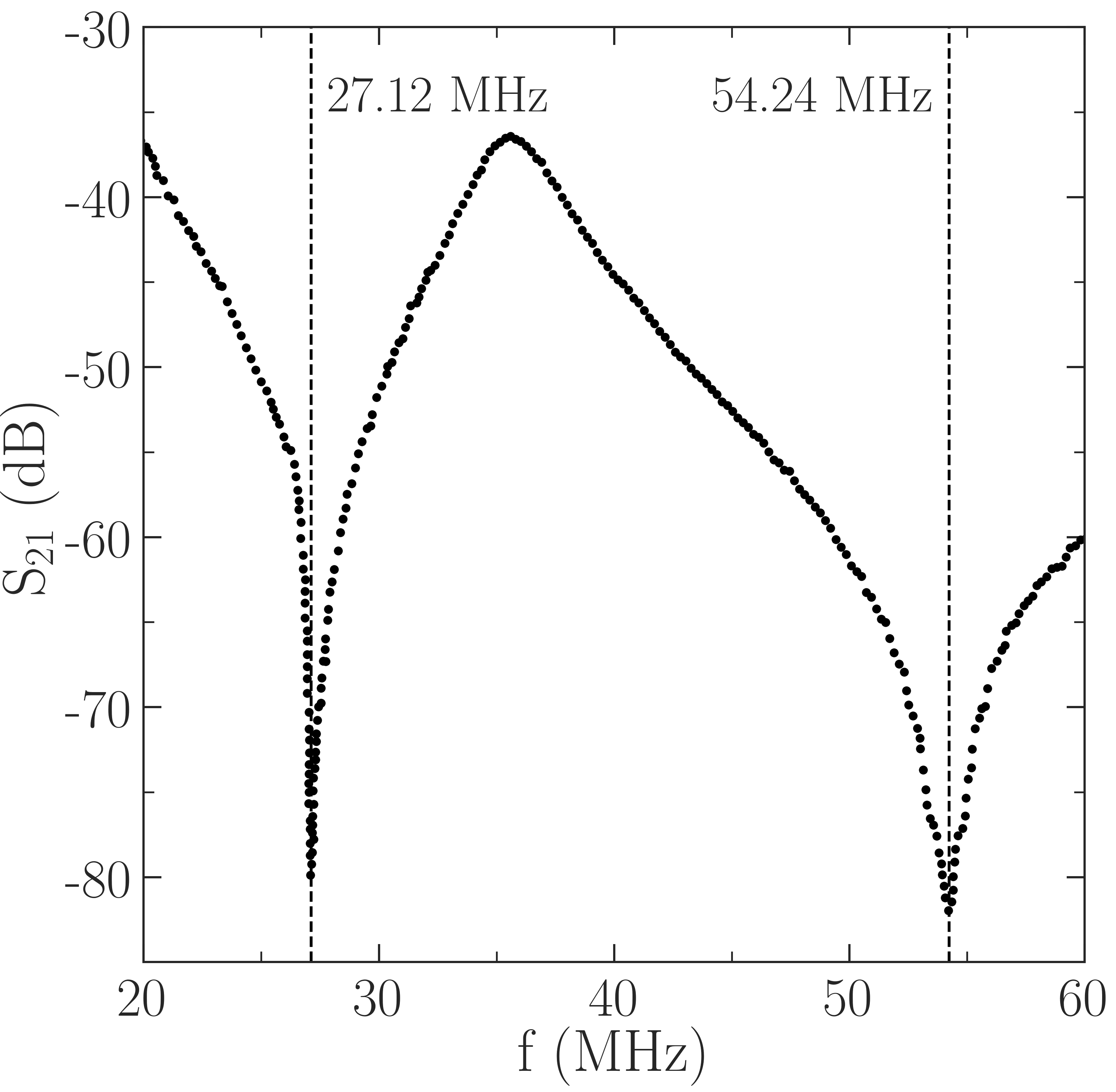
With the loop antenna capacitive coupling to the plasma, oscillations of the plasma potential at the applied radio-frequency and its harmonics are known to cause severe distortions to LP - characteristics Sudit and Chen (1994); Godyak and Demidov (2011). While this effect is not easily visible in the probe - characteristic, it becomes evident with the second derivative and, without proper mitigation, it severly compromises EEDF studies. Because the root-mean-square of at the first and second harmonics are larger than in the present apparatus, RF compensation was added to the Langmuir probe, following design steps described in detail in Sudit and Chen (1994) and Godyak and Demidov (2011). Four resonant chokes (TE Connectivity SC30100KT) and a reference electrode were incorporated in the probe head. The chokes self-resonant frequencies (SFR) were tuned to MHz and MHz with shunt capacitors of approriate values. The filter is housed inside the glass pipette, placed as close as possible to the probe tip to minimize stray capacitance. Shown in Fig. 1, the attenuation spectrum of the completed probe is checked with a spectrum analyzer for eventual detuning induced by the housing and adjacent wiring. The achieved attenuation of at least dB at the first and second harmonics provides sufficient filter impedance to suppress the RF oscillations. The reference electrode, connected to the probe tip through a capacitor, reduces the probe sheath impedance to ensure that the measuring tip follows the the plasma potential RF oscillations. For chokes containing ferrite cores, care should be taken to ensure that the ferrite does not saturate under the applied magnetic field or else the SFR will be shifted. The chokes employed were confirmed to be unaffected at the applied magnetic field strength of 300 G. The maximum probe biasing voltage was adjusted to V to avoid excessive electron current collection which could damage the probe tip or modify its work function. Tip contamination effects were monitored by checking for hysteresis in the up and down sweeps of . Probe cleaning by ion bombardment was used when necessary.
II.4 Data Collection
The Langmuir probe is mounted on a movable doglegged eccentric dielectric shaft which can span the entire length of the plasma source tube Filleul et al. (2021). The RFEA is mounted on a movable (rotation and translation) 6.35 mm diameter steel shaft introduced in the top port of the expansion chamber, with the probe orifice facing the plasma source exit to detect any possible directional ion beam. The LP current is deduced by measuring the voltage drop across a resistor with an isolation amplifier. The output of the amplifier is then split and fed into both a data acquisition system (DAQ) for digitization, and into an analog differentiator which outputs the first and second time derivatives. The LP and the RFEA are defined by several periods of a triangle wave function. The data acquisition is triggered by the output on the function generator to ensure signal synchronicity and the voltages are digitized at samples per period. One LP measurement is the average of sweeps, while one RFEA measurement averages sweeps.
III Data Processing Methods
Obtaining an accurate IEDF or EEDF requires choosing between different techniques to compute the first and second derivative of the - characteristics. An ideal method would provide an undistorted derivative with a signal-to-noise ratio (S/N) equal or lower to the raw data S/N. However, in practice there is a trade-off between noise level reduction and data distortion. Fortunately, analog and numerical methods can typically combine both noise filtering and differentiation of the raw - data. Some of the most commonly used numerical routines are presented in this section: the Savitzky-Golay filter, the B-spline fitting, the Gaussian and the Blackman filters, together with an analog differentiation technique. The Gaussian deconvolution method to obtain IEDFs is also described.
III.1 Analog Differentiation
The use of analog differentiator circuits predates numerical differentiation methods, and they are still regularly employed for obtaining EEDFs and occasionally for IEDFs Godyak, Piejak, and Alexandrovich (1992b); Takahashi et al. (2009); Takahashi, Shida, and Fujiwara (2010); Boswell et al. (2015); Yadav et al. (2018). The active analog differentiator used in this study, designed to work with a sweeping frequency of Hz, follows the design described in Takahashi et al. (2010). Two cascading operational amplifiers (Renesas CA3140) are each tuned to resonate at Hz by adjusting the resistors and capacitors values. This results in a linear gain frequency increase of dB per decade up to the resonance frequency, i.e. input signals of frequencies up to Hz are time-differentiated. Beyond the resonance frequency, the circuit acts as an integrator as the gain linearly decreases until becoming less than unity at kHz. Therefore the analog differentiator configuration also works as a band-pass filter, attenuating high frequency noise. Since real-world circuits deviate from the ideal-case, the linearity was checked to be strictly valid up to at least Hz. Each stage of the analog differentiator gives an output proportional to the first and second time derivative of the probe signal. Knowing the biasing/discriminator voltage sweep period and voltage swing, the differentiator output can be multiplied by to retrieve the derivative. Differentiator circuits have the advantage of producing repeatable outputs since no tuning of parameters for different experimental conditions are needed. This simplifies and speeds up the data processing.
III.2 Polynomial Methods
A polynomial least-squares regression to model the data using a single polynomial of degree via a least squares method has been previously attempted, giving poor results Magnus and Gudmundsson (2008). Since the - characteristics of interest can be visualized as part exponential and part linear, a single polynomial regression would require a high order to fit the data to a satisfactory level, e.g. , with the polynomial degree Magnus and Gudmundsson (2008). This leads to Runge’s phenomenon and over-fitting Celant and Broniatowski (7 62), which is visible in the results presented by Magnus and Gudmundsson (2008). Another shortcoming is the non-locality of the polynomial fit, i.e. distant data points directly impact the local fit Perperoglou et al. (2019). The SG filter and the B-spline methods both circumvent these problems by fitting low degree polynomials to subsets of the data.
III.2.1 Savitzky-Golay Filter
The Savitzky-Golay filter is frequently used for smoothing and differentiating current-voltage characteristics of Langmuir probes and RFEAs Xu and Walker (2012); Bétchu et al. (2013); Gulbrandsen and Fredriksen (2017); Damba et al. (2018). The filtering is achieved by doing a running fitting of a polynomial of degree using the least-squares method on a subset of the experimental data of width centered around a given point (forcing to strictly be an odd number). Evaluating the resulting polynomial at gives the smoothed value and the process is repeated for etc. Owing to the nature of this process, the first and last data points should be disregarded or the original data-set extrapolated by extra points at both ends.
Savitzky and Golay (1964) showed that for equally spaced data points, an analytical solution to the least-squares polynomial smoothing exists. Each one of the coefficients of the least-squares polynomial fitting is computed as a linear combination of the data points inside the subset of width . It was further demonstrated that the coefficients of the linear combinations are function of only. These can be tabulated for all pairs and applying the filter only requires convolution of the coefficients with the raw data Savitzky and Golay (1964). A benefit of this property is that the smoothed signal can be differentiated times by convolution with the derivative of the fitting polynomial, i.e. with the appropriate convolution coefficients Luo et al. (2005). This avoids having to recourse to numerical finite difference methods which tend to decrease the S/N. This can be understood by considering that the differential operator in the frequency domain is proportional to the frequency itself. For a given , the pairs , , , etc. give the same convolution coefficients for smoothing the raw data and evaluating the even derivatives, while , , give the same coefficients for odd derivatives Luo et al. (2005). Therefore for a given , using gives an identically smoothed derivative as using .
The SG filter acts as a low-pass filter with a flat passband whose cut-off frequency is a function of and . The cut-off frequency typically increases with and decreases with Luo et al. (2005). For large , the benefit of lower cut-off frequencies is compromised by distortions of the higher frequency content of the data. On the other hand, a large can preserve the narrow features of a signal (such as peaks) but at the cost of increasing the cut-off frequency Press and Teukolsky (1990). Obtaining an optimal filtering therefore requires an iterative process and a trade-off between the values of and .
III.2.2 B-spline Fitting
The piecewise polynomial approach used for data smoothing is the cardinal or uniform B-spline method De Boor and De Boor (2001). This polynomial fitting method avoids Runge’s phenonenon by making use of a piecewise approach: the data is split in pieces joined by equidistant points called knots. Like other polynomial regressions, the fitting polynomial , or spline function, of degree can be expressed as a linear combination of coefficients and basis functions (polynomials) :
| (5) |
Spline functions can therefore be calculated on different bases and the B-spline is a particular case for basis functions with local support, i.e. taking non-zero values only inside the interval on which they are defined, which spans knots. As a result, this method results in a higher numerical stability compared to other splines Perperoglou et al. (2019). The spline function is fitted to the data by using the least-square principle to calculate the coefficients . Additionally, the continuity conditions need to be verified, such that the function is times differentiable at the knots and that at the endpoints. The larger the number of knots, the higher the accuracy of the data fitting. However, more knots may result in over-fitting and/or poor noise rejection. A small number of knots could also over-smooth the data. As for the SG filter, the first and second derivatives of can be analytically derived.
III.3 Window Filters
III.3.1 Gaussian Filter
The Gaussian filter was developed by Hayden (1987) who introduced a new smoothing routine involving the use of a Gaussian distribution function as a filter. Fernández Palop et al. (1995) and Magnus and Gudmundsson (2008) used this algorithm to smooth the - characteristics measured with a Langmuir probe and obtain the electron-energy probability function. The working principle of the Gaussian filter is based on the assumption that the response function of the instrument and its electronics can be approximated as a Gaussian distribution with a given standard deviation :
| (6) |
The measured signal can then be calculated from the convolution of the experimental data with (). Because the noise is not correlated with the instrument response function, can be used for noise suppression. Owing to the property , the raw data can be convolved with the first and second derivative of the Gaussian function in order to obtain the first and second derivative of the - characteristic instead of using the central difference method. Nevertheless, for the sake of comparison with earlier results Magnus and Gudmundsson (2008), the central difference method was used to evaluate the derivatives.
III.3.2 Blackman Window Filter
The Blackman window is a standard moving average window, having zero value outside a chosen interval. It has been previously used to filter - characteristics in EEPF applications by Magnus and Gudmundsson (2008) and Roh et al. (2015). The Blackman window is defined by only one filtering parameter, i.e. the window size :
| (7) |
It is characterised by the highest reduction in the sidelobe level (down to dB) when compared to the other window functions (e.g. Hanning) Chassaing (2005). However, it has a wider mainlobe resulting in a less sharp transition band in the passband of the filter that can be improved by choosing a wider window size. The derivatives cannot be obtained analytically for the Blackman window, thus a central difference operator was used after filtering the raw - data.
III.4 Gaussian Deconvolution
The Gaussian deconvolution method, or Gaussian fitting, has been used to obtain the ion-energy distribution function from the - characteristics measured by a retarding field energy analyzer Charles and Boswell (2004); Cox et al. (2008); Imai and Takahashi (2022). This involves an iterative process of integrating a Gaussian curve that models the ion-energy distribution function until the raw - data are reconstructed. The fitting can either be manual, or an automatic Gaussian fitting algorithm can be implemented that minimises the sum of the squared errors between the measured and the reconstructed data.
For a single ion population, the ion-energy distribution function can be modeled with a Gaussian curve
| (8) |
where the parameters to be fit are: the amplitude , the curve width , and the location of the Gaussian peak . When a second ion population is present, as in the case of an accelerated ion beam in a collisional plasma, the IEDF requires the fitting of two or three Gaussian curves which are summed to accurately model the measured - curve Charles and Boswell (2004); Bennet, Charles, and Boswell (2018). An advantage of this technique is that it does not involve any filtering or differentiation steps since the IEDF is obtained in a retrograde approach.
IV Example of Application on a Data Set
IV.1 Optimization of Numerical Methods
The optimal evaluation of the ion and/or energy distribution functions through numerical methods requires a compromise in the choice of parameters to achieve sufficient noise-reduction without causing significant distortion of the fitted - characteristics that could lead to large errors in the inferred plasma parameters and loss of information.
An analysis similar to that used by Fernández Palop et al. (1995) and Magnus and Gudmundsson (2008) is used to assess the numerical methods in this work. It is noted that in Ref. Fernández Palop et al., 1995 and Ref. Magnus and Gudmundsson, 2008, the comparison of the different techniques was conducted on simulated - characteristics, while in this study only experimental data are used. The following parameters, evaluated between the raw probe collected current and the processed data , were considered: the mean squared error (MSE) and the Shapiro-Wilk (SW) test statistic .
When comparing different regression models, an optimal processing technique would return the lowest mean squared error. However, because the MSE value can range between zero and any larger number depending on the scale of the variables, it does not provide a standardized metric to assess how well the processing actually models the observed data. Moreover, the MSE on its own does not provide a way to highlight under-smoothing and over-fitting as these situations could return the lowest possible MSE. Thus, an analysis of the distribution of the residuals () is necessary to complement the MSE. In particular, verifying that the residuals are normally distributed ensures that the data processing does not significantly distort the - features Sen and Sen (1990). The Shapiro-Wilk test checks the null-hypothesis that the residuals are normally distributed by comparing the computed statistic with tabulated values Shapiro and Wilk (1965); Rahman and Govindarajulu (1997). For a given significance level, if is smaller than the tabulated value then the null-hypothesis can be rejected, i.e. the residuals are not normally distributed. Since filtering and fitting always somewhat distorts the data, one should aim to maximize and re-evaluate the data processing when the null-hypothesis is rejected. Taking a 0.01 significance level and given the samples size used in this study, the null-hypothesis is rejected if Rahman and Govindarajulu (1997). Therefore, a parametric analysis is conducted together with a visual optimization of the IEDF and EEPF for determining the optimal parameters for each numerical method. The assessment requires a trade-off between minimizing the MSE, maximizing and minimizing alterations of the raw - characteristic features.
| MSE | |||
| 3 | 5 | 0.9935 | |
| 3 | 15 | 0.9989 | |
| 3 | 35 | 0.9985 | |
| 3 | 80 | 0.9985 | |
| 2 | 15 | 0.9987 | |
| 4 | 15 | 0.9986 |

Specifically, the optimization of the IEDFs involves the careful computation of the first and second peak of the energy distributions, while achieving enough noise reduction when evaluating . An excessive smoothing of the - characteristics would modify the voltage at which the - curves present the gradient changes that corresponds to the center of two ion populations present. In turn, this would yield an incorrect evaluation of the plasma and ion beam potentials, and an inaccurate derivation of the ion-energy distribution. The dependency of the choice of the numerical processing parameters on the quality of the ion-energy distribution function was studied for each numerical method. Figure 2 shows an example of the effect of the parameter choices on the first derivative for different values of polynomial degree and number of knots using the B-spline technique. The mean-squared error and the Shapiro-Wilk test are evaluated for each case, and the values are reported in Table 1. When analyzing the dependence of the fitted polynomial degree while is kept constant, the MSE is seen to increase with , to decrease and the floor ripple level to increase (the Runge phenomenon). Since the obtained from a B-spline of degree is continuously differentiable, a quadratic B-spline does not provide a smooth first derivative (see Fig. 2 (a)). By extension, is the lowest B-spline degree that can be used to obtain a smooth second derivative for the EEPF. If the number of knots is too small the evaluated IEDF is over-smoothed and the features of the - characteristic are distorted ( for and ). In contrast, as shown in Fig. 2 (f), too high a number of knots causes an insufficient smoothing of the noise, which could make it difficult to determine the location of the peaks. For the data analyzed in this study, a degree of and a number of knots are chosen for the B-spline polynomial since they result in the optimal IEDF i.e., lowest curve distortion and sufficient noise reduction.

| MSE | |||
| 2 | 51 | 0.9973 | |
| 2 | 91 | 0.9961 | |
| 2 | 115 | 0.9964 | |
| 2 | 251 | 0.7135 | |
| 4 | 251 | 0.9132 | |
| 6 | 251 | 0.9937 |
Similarly, optimal evaluation of the EEDFs requires simultaneously maximizing the energy resolution and the dynamic range (DR). The energy resolution is characterized by the low-energy depletion which is defined as the value of the maximum of the EEDF. Because the bulk of the electrons are in the low-energy region of the EEPF, the larger , the larger the errors in determining and from Eq. 3 and Eq. 4. An EEDF is considered to have sufficient energy resolution if Godyak and Demidov (2011); Godyak (2021). The dynamic range of the EEPF is defined as the ratio of its maximum to its minimum resolvable value. A dynamic range dB (equivalently of 3 orders of magnitude and above) is necessary to resolve high-energy electrons in the inelastic range of the EEPF, which are detrimental in investigating excitation, ionization, and transport processes Godyak and Demidov (2011); Godyak (2021). An EEDF is often separated into its elastic and inelastic ranges, defined as and , respectively. is the lowest excitation energy of the working gas, e.g. 11.55 eV for argon Puech and Torchin (1986). Minimizing and maximizing the DR is therefore paramount in the process of determining the optimal numerical parameters, together with minimizing the MSE and maximizing the value of .
Figure 3 shows an example of the impact of varying the polynomial degree and moving window size of the Savitzky-Golay filter when applied to a compensated LP - characteristic acquired with the experimental apparatus. For each pair, the corresponding MSE and Shapiro-Wilk test statistic are given in Table 2. In Fig. 3 (a)-(d) , and the effect of increasing is shown. As expected for an SG filter, increasing is beneficial from the dynamic range point-of-view since it improves from 13 dB to 46 dB owing to the decreasing cut-off frequency. However, this is accompanied by distortions of the signal, visible from the worsening of the low-energy resolution , the MSE and . Fixing and increasing to the next even integers (since and produce the same output), the signal distortion improves again at the cost of decreasing the DR, as shown in Fig. 3 (d)-(f) and Table 2. Regarding the Shapiro-Wilk test, all the cases with failed the normality test with . Overall, trading-off between , the DR, the MSE and , the best performing filter for this data is for . It is noted that none of the pairs produced an EEPF fulfilling the aforementioned requirements, since the dynamic range never reaches 3 orders of magnitude. Different pairs can be used whether the goal of obtaining the EEPF lies in the study of elastic or inelastic processes. Alternatively, the outputs of two SG filter applications could be combined into a high resolution and high dynamic range numerically derived EEPF, with the drawback of a more complicated post-processing Roh et al. (2015).
IV.2 Ion-Energy Distribution Function (IEDF)
As mentioned in Section I, the ion-energy distribution function can be derived from the first derivative of the measurements acquired with a retarding field energy analyzer. The respective - characteristics was taken in the expansion chamber with the RFEA orifice located 19 cm downstream of the magnetic nozzle ( cm). The experimental conditions were maintained at an RF power of W, argon pressure in the chamber of mTorr, and a maximum magnetic field on axis of G. Under these conditions, the plasma density peaks axially under the solenoids reaching a value of which then decreases to in the expansion chamber. The data processing of the collected current measured with the energy analyzer and the subsequent computation of the ion-energy distribution function followed the approach described in Section IV.1.
Table 4 summarizes the results of the parametric analysis that provide the smoothest IEDF possible for the numerical smoothing methods analyzed, while keeping intact the peak features. Figure 4 shows the ion-energy distribution functions obtained with the different analog and numerical techniques from experimental data. The IEDFs plotted are normalized by their peak value, and the position of the two peaks, i.e. the local plasma potential and the ion beam potential, is also reported. The data in Fig. 4 has a signal-to-noise ratio of approximately dB. The raw - curve, shown in Fig. 4 (a), was obtained by averaging 200 consecutive probe sweeps and it is plotted with the fitted Gaussian deconvolution to illustrate one of the data processing methods. As seen in Fig. 4, the ion-energy distribution functions show a double-peak feature indicating the presence of a bi-population of ions: the first peak represents the background ion population (at zero energy) which location can be considered the local plasma potential , while the second peak corresponds to the accelerated ion beam population with potential end energy . Comparing measurements taken with a source-facing and a radial-facing RFEA shows that the IEDF does not present a peak separation effect due to RF modulation, but it effectively detects the presence of a directional ion beam Caldarelli et al. (2022). It is also noted that the ion-neutral mean free path for the operating pressure of mTorr is shorter than the distance between the source exit and the probe position i.e., cm and cm. Thus, the accelerated ion beam component is decreased at the measurement location while the local, background ion population is enhanced due to charge-exchange collisions. Furthermore, elastic collisions could affect the beam direction, further reducing the collected beam current.
Table 3 presents the key results obtained with the different data processing techniques, namely: the local plasma potential , the ion beam potential , the mean squared error (MSE), and the Shapiro-Wilk test statistic . The Gaussian deconvolution method required the fitting of three Gaussian curves to accurately model the two ion populations.

| Method | (V) | (V) | MSE | |
|---|---|---|---|---|
| Analog | 21.03 | 39.02 | - | - |
| Gaussian deconv. | 20.94 | 39.07 | 0.9990 | |
| SG | 20.90 | 39.07 | 0.9986 | |
| B-spline | 20.58 | 39.03 | 0.9989 | |
| GF | 21.16 | 38.61 | 0.9984 | |
| BW | 21.16 | 38.61 | 0.9984 |
| Method | Differentiation | Window size | Degree | Sigma | Knots | ||||
|---|---|---|---|---|---|---|---|---|---|
| EEPF | IEDF | EEPF | IEDF | EEPF | IEDF | EEPF | IEDF | ||
| Savitzky-Golay Filter | Analytic | - | - | - | - | ||||
| B-spline Fitting | Analytic | - | - | - | - | ||||
| Gaussian Filter | Analytic | - | - | - | - | - | - | ||
| Blackman Window | Central Difference | - | - | - | - | - | - | ||
Comparing the analog differentiation method and the numerical techniques, it is evident that both the plasma and ion beam potentials are approximately unchanged with a standard deviations for and of V and V, respectively. For the collected data, all the smoothing methods perform well in terms of mean squared error and the SW test statistic. The MSEs are for all techniques, while the calculated values are all higher than 0.998. The Saviztky-Golay filter yields the lowest MSE, while the Gaussian deconvolution methods performs the best in the SW test, resulting in the highest . It has to be noted that the Blackman filter showed an overshoot of the fitted polynomial at the edges caused by the zero padding in the convolution; this was addressed by disregarding the initial data points as the plasma characteristics in that region were not of interest.
IV.3 Electron-Energy Probability Function (EEPF)
The RF compensated LP data were acquired with the apparatus operated at W of RF power, mTorr of argon, G and with the Helmholtz solenoids placed 30 cm away from the loop antenna. These conditions create an inductively coupled plasma exhibiting a symmetrical single peaked axial plasma density gradient ranging from under the solenoids to at the extremities of the glass tube Filleul et al. (2021, 2022); Bennet, Charles, and Boswell (2019). The LP was placed on axis halfway between the antenna and the solenoids. The processing of to obtain the EEPF with the analog and numerical methods was conducted following the steps described in Section IV.1. Table 4 gives the resulting optimal numerical parameters.
Figure 5 (a) shows the raw - LP characteristic together with the optimized Savitkzy-Golay filter output from Fig. 3, i.e. for . As reference, the signal-to-noise ratio of the LP characteristic is dB. In Fig. 5 (b)-(f), the EEPFs obtained from the various methods and the deduced plasma parameters are shown. and are calculated by integrating the EEPF according to Eq. 4 and Eq. 3, respectively. Their values are reported together with , the MSE, , dynamic range and energy resolution for each method in Table 5. The maximum variance in the obtained values of is less than 2. Likewise, for and , their maximum variances are and , respectively. Thus, in terms of estimating the plasma parameters, all 5 methods have comparable performance, i.e. within the absolute error tolerances usually associated with LP measurements Boswell et al. (2015); Godyak (2021).

| Method | (V) | (eV) | MSE | DR (dB) | (eV) | ||
|---|---|---|---|---|---|---|---|
| Analog | 68.08 | 5.65 | 1.87 | - | - | 55 | 3.2 |
| SG | 67.14 | 5.52 | 1.85 | 0.91 | 0.9964 | 32 | 3.4 |
| B-spline | 66.95 | 5.21 | 1.76 | 0.84 | 0.997 | 36 | 2.3 |
| GF | 67.01 | 5.97 | 1.85 | 3.3 | 0.8015 | 33 | 3.4 |
| BW | 67.08 | 5.38 | 1.91 | 3.1 | 0.8537 | 33 | 3.5 |
In terms of energy resolution and dynamic range, different methods perform best depending on whether the focus is on resolving low-energy or high-energy electrons dynamics and properties. The B-spline fitting in Fig. 5 (d) resulted in the best energy resolution at eV and is the only method to satisfy the condition. The second-best performing method is the analog differentiation with eV, i.e. 0.375 eV away from satisfying the energy resolution condition. Regardless of the employed method, the energy resolution is ultimately limited by the absence of internal resistance compensation in the present LP implementation, in particular of the plasma-wall sheath impedance, or by the probe tip surface condition Godyak (2021). Techniques to further improve the resolution are available in Ref. Roh et al., 2015; Godyak, 2021.
The analog differentiation method in Fig. 5 (b) resulted in an EEPF with a significantly larger dynamic range of approximately 3 orders of magnitude, compared to 2 orders of magnitude for the numerical methods. The analog differentiation is therefore the only method presented which can reliably resolve inelastic processes and can provide confidence on the nature of the electron distribution function, i.e. a single-Maxwellian for up to 30 eV in the present case. This is further highlighted in Fig. 5 (b) by the linear regression of the EEPF, shown by a dashed red line. The same linear regression applied to the numerically derived EEPFs highlights that the reduced DR and artificial oscillations in the case of the B-spline would make it difficult to reach conclusions on the nature of the electron distribution function. Among the numerical methods, the Savitzky-Golay and the B-spline are the best performing for this data set, with the lowest distortion of the original - curve, as shown by their lower mean-square errors and Shapiro-Wilk test statistics in Table 5. The Gaussian and Blackman window filters both resulted in noticeable distortions of the data (, i.e. their residuals are not normally distributed), in particular around the plasma floating potential and plasma potential portions of the - curve.
Finally, it is interesting to note that following the guidelines in Ref. Godyak, 2021, the low-energy gap impacts can be corrected by extrapolating the EEPF from its linear portion down to eV when the right conditions are satisfied. Because electron-electron collisions are the dominant processes for thermalizing electrons and making the distribution Maxwellian, and since the frequency of these collisions is inversely proportional to , if the EEPF is Maxwellian for some greater than the energy of EEPF peak, then the EEPF is likely to be Maxwellian at lower energies Tsendin (2009); Kaganovich et al. (2009); Godyak (2021). This extrapolation can be achieved with the linear regressions shown in Fig. 5 as dashed red curves. Applying this process to the analog EEPF in Fig. 5 (b) for example, the effective electron temperature obtained with the corrected EEPF is eV and the corrected electron density , to compare with the values in Table 5. The electron temperature obtained from the slope of the linear regression is eV, providing evidence that the low-energy extrapolation has closely recovered the original EEPF shape.
V Conclusions
This review outlines some of the most frequently employed data processing methods to obtain ion and electron-energy distribution functions from - characteristics measured with a retarding field energy analyzer and an RF compensated Langmuir probe, respectively. Design recommendations relevant to measurements in RF magnetized plasmas are presented for both instruments. After describing the different processing techniques, an example of a parametric analysis to obtain optimal IEDFs and EEPFs is presented and applied to experimental data sets collected in a magnetized RF plasma apparatus. The recommended parameters optimization involves checking the mean-squared error and the normal distribution of the residuals (i.e. the Shapiro-Wilk test), coupled with a visual assessment process to ensure sufficient noise reduction with minimal distortion of the curves.
With respect to the IEDF, the analysis focused on the evaluation of first derivatives that accurately represented a plasma containing a bi-population of ions. For the data set under study, both the analog and numerical methods provide smooth IEDFs and consistent values of the local plasma and the ion beam potentials. Regarding the numerical methods analyzed, they all perform well in terms of MSE and ; in particular, the Saviztky-Golay filter and the Gaussian deconvolution methods delivered the best results in terms of obtaining accurate IEDFs with the least data distortion.
The EEPFs obtained from each method are assessed in terms of maximizing the energy resolution and dynamic range while minimizing distortions of the Langmuir probe - curve. Among the numerical methods, the Savitzky-Golay filter and the B-spline fitting performed best in terms of distortion and energy resolution. All numerical methods delivered a mediocre dynamic range of approximately 2 orders of magnitude, which is to be related to the experimental data set employed having a low signal-to-noise ratio of dB. This could make it challenging to confidently identify the nature of the electron distribution function and to study inelastic electron processes. This is in contrast with the EEPF obtained from the same - curve using the analog differentiator which showed a dynamic range of approximately 3 orders of magnitude and can be clearly identified as being Maxwellian up to eV. When the intent of calculating the EEPF is solely to obtain the plasma parameters, all methods explored are found to deliver equivalent results. The analog differentiator technique provides an appreciable reduction in the IEDF and EEPF processing time compared to the numerical methods since no data-set specific optimization is required.
Data Availability Statement
The data that support the findings of this study are available from the corresponding author upon reasonable request.
Author Contributions
In alphabetical order, A.C. and F.F. share first authorship. A.C. and F.F. performed the data acquisition, data processing and manuscript preparation concerning the IEDF and EEDF, respectively. R.B. and C.C. provided guidance in experimental RF plasmas and diagnostics. N.R. and J.C. are doctoral supervisors of A.C. and F.F.
Conflict of Interest Statement
The authors declare that the research was conducted in the absence of any commercial or financial relationships that could be construed as a potential conflict of interest.
References
- Godyak, Piejak, and Alexandrovich (1993) V. Godyak, R. Piejak, and B. Alexandrovich, “Probe diagnostics of non-Maxwellian plasmas,” Journal of Applied Physics 73, 3657–3663 (1993).
- Charles and Boswell (2004) C. Charles and R. Boswell, “Laboratory evidence of a supersonic ion beam generated by a current-free “helicon” double-layer,” Physics of Plasmas 11, 1706–1714 (2004).
- Takahashi et al. (2009) K. Takahashi, C. Charles, R. Boswell, W. Cox, and R. Hatakeyama, “Transport of energetic electrons in a magnetically expanding helicon double layer plasma,” Applied Physics Letters 94, 191503 (2009).
- Boswell et al. (2015) R. W. Boswell, K. Takahashi, C. Charles, and I. D. Kaganovich, “Non-local electron energy probability function in a plasma expanding along a magnetic nozzle,” Frontiers in Physics 3, 14 (2015).
- Ingram and Braithwaite (1988) S. Ingram and N. S. J. Braithwaite, “Ion and electron energy analysis at a surface in an RF discharge,” Journal of Physics D: Applied Physics 21, 1496 (1988).
- Habl, Rafalskyi, and Lafleur (2020) L. Habl, D. Rafalskyi, and T. Lafleur, “Ion beam diagnostic for the assessment of miniaturized electric propulsion systems,” Review of Scientific Instruments 91, 093501 (2020).
- Godyak, Piejak, and Alexandrovich (1992a) V. Godyak, R. Piejak, and B. Alexandrovich, “Evolution of the electron-energy-distribution function during rf discharge transition to the high-voltage mode,” Physical Review Letters 68, 40 (1992a).
- Takahashi et al. (2020) K. Takahashi, C. Charles, R. W. Boswell, and A. Ando, “Thermodynamic analogy for electrons interacting with a magnetic nozzle,” Physical Review Letters 125, 165001 (2020).
- Mott-Smith and Langmuir (1926) H. M. Mott-Smith and I. Langmuir, “The theory of collectors in gaseous discharges,” Physical Review 28, 727 (1926).
- Merlino (2007) R. L. Merlino, “Understanding Langmuir probe current-voltage characteristics,” American Journal of Physics 75, 1078–1085 (2007).
- Godyak and Demidov (2011) V. Godyak and V. Demidov, “Probe measurements of electron-energy distributions in plasmas: what can we measure and how can we achieve reliable results?” Journal of Physics D: Applied Physics 44, 233001 (2011).
- Godyak (2021) V. Godyak, “RF discharge diagnostics: Some problems and their resolution,” Journal of Applied Physics 129, 041101 (2021).
- Druyvesteyn (1930) M. J. Druyvesteyn, “Der niedervoltbogen,” Zeitschrift für Physik 64, 781–798 (1930).
- Böhm and Perrin (1993) C. Böhm and J. Perrin, “Retarding-field analyzer for measurements of ion energy distributions and secondary electron emission coefficients in low-pressure radio frequency discharges,” Review of Scientific Instruments 64, 31–44 (1993).
- Charles et al. (2000) C. Charles, A. W. Degeling, T. E. Sheridan, J. H. Harris, M. A. Lieberman, and R. W. Boswell, “Absolute measurements and modeling of radio frequency electric fields using a retarding field energy analyzer,” Physics of Plasmas 7, 5232–5241 (2000).
- Cox et al. (2008) W. Cox, C. Charles, R. W. Boswell, and R. Hawkins, “Spatial retarding field energy analyzer measurements downstream of a helicon double layer plasma,” Applied Physics Letters 93, 071505 (2008).
- Takahashi, Shida, and Fujiwara (2010) K. Takahashi, Y. Shida, and T. Fujiwara, “Magnetic-field-induced enhancement of ion beam energy in a magnetically expanding plasma using permanent magnets,” Plasma Sources Science and Technology 19, 025004 (2010).
- Bennet, Charles, and Boswell (2018) A. Bennet, C. Charles, and R. Boswell, “In situ electrostatic characterisation of ion beams in the region of ion acceleration,” Physics of Plasmas 25, 023516 (2018).
- Imai and Takahashi (2022) R. Imai and K. Takahashi, “Deflections of dynamic momentum flux and electron diamagnetic thrust in a magnetically steered rf plasma thruster,” Journal of Physics D: Applied Physics 55, 135201 (2022).
- Keesee et al. (2005) A. M. Keesee, E. E. Scime, C. Charles, A. Meige, and R. Boswell, “The ion velocity distribution function in a current-free double layer,” Physics of Plasmas 12, 093502 (2005).
- Savitzky and Golay (1964) A. Savitzky and M. J. E. Golay, “Smoothing and Differentiation of Data by Simplified Least Squares Procedures.” Analytical Chemistry 36, 1627–1639 (1964).
- Sudit and Woods (1993) I. D. Sudit and R. C. Woods, “A workstation based Langmuir probe system for low-pressure dc plasmas,” Review of Scientific Instruments 64, 2440–2448 (1993).
- Bétchu et al. (2013) S. Bétchu, A. Soum-Glaude, A. Bès, A. Lacoste, P. Svarnas, S. Aleiferis, A. Ivanov Jr, and M. Bacal, “Multi-dipolar microwave plasmas and their application to negative ion production,” Physics of Plasmas 20, 101601 (2013).
- Conde et al. (2017) L. Conde, J. L. Domenech-Garret, J. M. Donoso, J. Damba, S. P. Tierno, E. Alamillo-Gamboa, and M. A. Castillo, “Supersonic plasma beams with controlled speed generated by the alternative low power hybrid ion engine (ALPHIE) for space propulsion,” Physics of Plasmas 24, 123514 (2017).
- Damba et al. (2018) J. Damba, P. Argente, P. Maldonado, A. Cervone, J.-L. Domenech-Garret, and L. Conde, “Multiprobe characterization of plasma flows for space propulsion,” Journal of Physics: Conference Series 958, 012002 (2018).
- Fernández Palop et al. (1995) J. Fernández Palop, J. Ballesteros, V. Colomer, and M. Hernández, “A new smoothing method for obtaining the electron energy distribution function in plasmas by the numerical differentiation of the I-V probe characteristic,” Review of Scientific Instruments 66, 4625–4636 (1995).
- Magnus and Gudmundsson (2008) F. Magnus and J. T. Gudmundsson, “Digital smoothing of the Langmuir probe I-V characteristic,” Review of Scientific Instruments 79, 073503 (2008).
- Sloane and MacGregor (1934) R. Sloane and E. MacGregor, “An alternating current method for collector analysis of discharge-tubes,” The London, Edinburgh, and Dublin Philosophical Magazine and Journal of Science 18, 193–207 (1934).
- Godyak, Piejak, and Alexandrovich (1992b) V. Godyak, R. Piejak, and B. Alexandrovich, “Measurement of electron energy distribution in low-pressure rf discharges,” Plasma Sources Science and Technology 1, 36 (1992b).
- Yadav et al. (2018) S. Yadav, S. Ghosh, S. Bose, K. Barada, R. Pal, and P. Chattopadhyay, “Role of ion magnetization in formation of radial density profile in magnetically expanding plasma produced by helicon antenna,” Physics of Plasmas 25, 043518 (2018).
- Caldarelli et al. (2022) A. Caldarelli, F. Filleul, C. Charles, R. Boswell, N. Rattenbury, and J. Cater, “Radial characterization of an ion beam in a deflected magnetic nozzle,” Journal of Electric Propulsion 1, 10 (2022).
- Filleul et al. (2021) F. Filleul, A. Caldarelli, C. Charles, R. Boswell, N. Rattenbury, and J. Cater, “Characterization of a new variable magnetic field linear plasma device,” Physics of Plasmas 28, 123514 (2021).
- Filleul et al. (2022) F. Filleul, A. Caldarelli, R. Boswell, C. Charles, N. Rattenbury, and J. Cater, “The role of ion magnetization on plasma generation in a magnetic nozzle rf device,” Journal of Electric Propulsion 1, 20 (2022).
- Cox et al. (2010) W. Cox, C. Charles, R. W. Boswell, R. Laine, and M. Perren, “Magnetic ion beam deflection in the helicon double-layer thruster,” Journal of Propulsion and Power 26, 1045–1052 (2010).
- Caldarelli et al. (2021) A. Caldarelli, F. Filleul, C. Charles, N. Rattenbury, and J. Cater, “Preliminary Measurements of a Magnetic Steering System for RF Plasma Thruster Applications,” in AIAA Propulsion and Energy 2021 Forum (2021) p. 3401.
- Conway, Perry, and Boswell (1998) G. D. Conway, A. J. Perry, and R. W. Boswell, “Evolution of ion and electron energy distributions in pulsed helicon plasma discharges,” Plasma Sources Science and Technology 7, 337–347 (1998).
- Sudit and Chen (1994) I. D. Sudit and F. F. Chen, “RF compensated probes for high-density discharges,” Plasma Sources Science and Technology 3, 162 (1994).
- Takahashi et al. (2010) K. Takahashi, C. Charles, R. Boswell, M. A. Lieberman, and R. Hatakeyama, “Characterization of the temperature of free electrons diffusing from a magnetically expanding current-free double layer plasma,” Journal of Physics D: Applied Physics 43, 162001 (2010).
- Celant and Broniatowski (7 62) G. Celant and M. Broniatowski, Interpolation and Extrapolation Optimal Designs 1: Polynomial Regression and Approximation Theory (John Wiley & Sons, New York, 2016, pp. 57-62).
- Perperoglou et al. (2019) A. Perperoglou, W. Sauerbrei, M. Abrahamowicz, and M. Schmid, “A review of spline function procedures in R,” BMC Medical Research Methodology 19, 1–16 (2019).
- Xu and Walker (2012) K. G. Xu and M. L. Walker, “Plume Characterization of an Ion-Focusing Hall Thruster,” Journal of Propulsion and Power 28, 1105–1115 (2012).
- Gulbrandsen and Fredriksen (2017) N. Gulbrandsen and Å. Fredriksen, “RFEA Measurements of High-Energy Electrons in a Helicon Plasma Device with Expanding Magnetic Field,” Frontiers in Physics 5 (2017), 10.3389/fphy.2017.00002.
- Luo et al. (2005) J. Luo, K. Ying, P. He, and J. Bai, “Properties of Savitzky–Golay digital differentiators,” Digital Signal Processing 15, 122–136 (2005).
- Press and Teukolsky (1990) W. H. Press and S. A. Teukolsky, “Savitzky-Golay Smoothing Filters,” Computers in Physics 4, 669–672 (1990).
- De Boor and De Boor (2001) C. De Boor and C. De Boor, A practical guide to splines, Vol. 27 (Springer-Verlag New York, 2001).
- Hayden (1987) H. C. Hayden, “Data smoothing routine,” Computers in Physics 1, 74–75 (1987).
- Roh et al. (2015) H.-J. Roh, N.-K. Kim, S. Ryu, S. Park, S.-H. Lee, S.-R. Huh, and G.-H. Kim, “Determination of electron energy probability function in low-temperature plasmas from current - Voltage characteristics of two Langmuir probes filtered by Savitzky–Golay and Blackman window methods,” Current Applied Physics 15, 1173–1183 (2015).
- Chassaing (2005) R. Chassaing, Digital signal processing and applications with the C6713 and C6416 DSK (Wiley-Interscience, Hoboken, N.J., 2005).
- Sen and Sen (1990) A. K. Sen and A. Sen, Regression analysis : theory, methods and applications (Springer-Verlag, New York, 1990).
- Shapiro and Wilk (1965) S. S. Shapiro and M. B. Wilk, “An analysis of variance test for normality (complete samples),” Biometrika 52, 591–611 (1965).
- Rahman and Govindarajulu (1997) M. M. Rahman and Z. Govindarajulu, “A modification of the test of shapiro and wilk for normality,” Journal of Applied Statistics 24, 219–236 (1997).
- Puech and Torchin (1986) V. Puech and L. Torchin, “Collision cross sections and electron swarm parameters in argon,” Journal of Physics D: Applied Physics 19, 2309 (1986).
- Bennet, Charles, and Boswell (2019) A. Bennet, C. Charles, and R. Boswell, “Non-local plasma generation in a magnetic nozzle,” Physics of Plasmas 26, 072107 (2019).
- Tsendin (2009) L. Tsendin, “Electron kinetics in glows—from Langmuir to the present,” Plasma Sources Science and Technology 18, 014020 (2009).
- Kaganovich et al. (2009) I. Kaganovich, V. Demidov, S. Adams, and Y. Raitses, “Non-local collisionless and collisional electron transport in low-temperature plasma,” Plasma Physics and Controlled Fusion 51, 124003 (2009).