Data-driven modelling of nonlinear spatio-temporal fluid flows using a deep convolutional generative adversarial network
Abstract
Deep learning techniques for improving fluid flow modelling have gained significant attention in recent years. Advanced deep learning techniques achieve great progress in rapidly predicting fluid flows without prior knowledge of the underlying physical relationships. However, most of existing researches focused mainly on either sequence learning or spatial learning, rarely on both spatial and temporal dynamics of fluid flows (Reichstein et al., 2019). In this work, an Artificial Intelligence (AI) fluid model based on a general deep convolutional generative adversarial network (DCGAN) has been developed for predicting spatio-temporal flow distributions. In deep convolutional networks, the high-dimensional flows can be converted into the low-dimensional “latent” representations. The complex features of flow dynamics can be captured by the adversarial networks. The above DCGAN fluid model enables us to provide reasonable predictive accuracy of flow fields while maintaining a high computational efficiency. The performance of the DCGAN is illustrated for two test cases of Hokkaido tsunami with different incoming waves along the coastal line. It is demonstrated that the results from the DCGAN are comparable with those from the original high fidelity model (Fluidity). The spatio-temporal flow features have been represented as the flow evolves, especially, the wave phases and flow peaks can be captured accurately. In addition, the results illustrate that the online CPU cost is reduced by five orders of magnitude compared to the original high fidelity model simulations. The promising results show that the DCGAN can provide rapid and reliable spatio-temporal prediction for nonlinear fluid flows.
keywords:
Deep convolutional GAN, nonlinear fluid flow, data-driven modelling, deep learning1 Introduction
Numerical simulations of fluid dynamics have been indispensable in many applications relevant to physics and engineering. For improving predictive capability, numerical algorithms have become increasingly sophisticated and complicated by using more spatial and temporal resolution of datasets. This often leads to very large-scale models and unavoidably raises computational challenges. In this work, an Artificial Intelligence (AI) fluid flow model is presented for rapidly providing spatio-temporal prediction of nonlinear fluid flows while avoiding the excessive computational cost.
Recently, deep learning has gained popularity in rapidly predicting nonlinear fluid flows (Kalteh, 2013; Kasiviswanathan et al., 2016; Kisi et al., 2012; Lohani et al., 2014; Yang et al., 2017; Wang et al., 2018; Brunton et al., 2019). Deep learning techniques are capable to handle the large-scale data from the dynamic and nonlinear systems, and provide accurate nonlinear fluid flow prediction without prior knowledge of underlying physical relationships. Various deep learning techniques have been applied to nonlinear fluid flow prediction, for example, modifying the model parameters by Bayesian deep neural networks to enhance the flow prediction in the turbulence model (Geneva and Zabaras, 2019), obtaining the time-series streamflow prediction by Long Short-Term Memory (LSTM) networks (Hu et al., 2019a), and simulating unsteady wake flows by convolutional neural network (CNN) -based deep learning (Miyanawala and Jaiman, 2017).
More recently, Generative Adversarial Networks (GANs) have been introduced to reconstruction of fluid dynamic features (Farimani et al., 2017; Xie et al., 2018). GANs represent the most recent progress in deep learning techniques (Goodfellow, 2016; Laloy et al., 2017; Ströfer et al., 2018) and have been attractive for producing high-resolution samples (e.g. images) (Ledig et al., 2017; Xie et al., 2018; Creswell et al., 2018). The main specificity of GANs is the competition game between the generator and discriminator modules. The generator consists of deep neural networks, which can produce high-dimensional distributions of data to “fool” the discriminator. The discriminator is responsible for distinguishing the real data from the generated data. Nowadays applications of GANs focus mostly on images (Reed et al., 2016; Li and Wand, 2016; Isola et al., 2017), rarely on fluid flow problems (Farimani et al., 2017; Xie et al., 2018). Farimani et al. (2017) first introduced the conditional generative adversarial networks (cGAN) to simulate steady state heat conduction and incompressible fluid flow. This study proves that GANs can be effective in exhibiting complex nonlinear fluid structures. Xie et al. (2018) introduced a temporal discriminator to GANs for solving the super-resolution problem for smoke flows.
In this work, we have developed a deep convolutional generative adversarial network (DCGAN) (Radford et al., 2015) for nonlinear unsteady fluid flow problems. This is the first attempt to use the DCGAN for predictive analysis in fluid flow problems. As is well known, both spatially and temporally flow dynamic properties are important in prediction. Classic machine learning approaches exploit dependencies in time or space, rarely both spatio-temporal dependencies (Reichstein et al., 2019). Here, the DCGAN is first used to extract the spatio-temporal coherence of the original high-dimensional fluid fields. The high-dimensional nonlinear fluid flow features can be converted into low-dimensional “latent” representations. With discriminating the real fluid fields and their realizations in the low-dimensional latent space, the training process herein is fast. This alleviates the problem of large data-driven modelling. The way of dimensionality reduction in the deep convolutional networks is similar to that of Galerkin reduced order model (ROM) (Fang et al., 2013, 2014; Xiao et al., 2019), Variational Autoencoder (VAE) (Gonzalez and Balajewicz, 2018) and cluster-based reduced order model (CROM) (Kaiser et al., 2014; Nair et al., 2019; Östh et al., 2015). These ROMs are able to compress spatial-temporal flow snapshots into a small number of low-dimensional states for dynamic modelling, which is also a strategy to reduce computational requirements of ROMs (Kaiser et al., 2014). Nevertheless, the prominent difference between the DCGAN and existing ROMs lies in the fact that the CROM or POD based ROMs result in linear combinations of the original snapshots (Kaiser et al., 2014; Xiao et al., 2016), while the deep convolutional neural networks are able to capture the nonlinear flow transients since the effective basis functions are non-linear (Miyanawala and Jaiman, 2017). In addition, GAN also has the key advantage that, in principle, any point in the latent space of inputs will be associated with a realistic looking solution.
The DCGAN is a general and efficient numerical tool for rapidly predicting nonlinear fluid flows for given inputs. In this work, we have successfully applied the DCGAN to a tsunami case in the southwestern Hokkaido Island, Japan. The performance of the DCGAN has been evaluated by comparing the results obtained with those from an unstructured mesh finite element model (Fluidity) (Pain et al., 2001).
The structure of this article is organized as follows. Section 2 presents the governing equation for nonlinear fluid flows in dynamic systems. The architecture of the DCGAN is briefly introduced in section 3. The detailed process for the large data-driven modelling is described in section 4. Section 5 illustrates the capability of the DCGAN in the tsunami case, which entails the snapshot-based datasets generation with the different wave characteristics and the DCGAN training. Results of cases and the model efficiency are then presented in section 6. Conclusions are drawn in section 7.
2 Governing equations for nonlinear fluid flow prediction problems
Nonlinear fluid flows are usually simulated by solving the complex non-linear equations (for example, Navier-Stokes (NS) equations, Lorenz equations and shallow water equations) in the computational fluid dynamic models. In a general way, the governing equation of dynamic flows can be expressed as:
| (1) |
where is the state variable to be predicted (for example, water depth and velocity), represents the inputs (for example, initial and boundary conditions, modelling parameters) , denotes the spatial coordinate system, is the source term, and is the time.
This work focuses on the spatio-temporal fluid simulations that are driven by the inputs (for example, initial and boundary conditions, modelling parameters). The nonlinear relationship between the fluid flow solutions and the inputs in Eq.(1) can be re-written in a general way:
| (2) |
where represents a dynamic model. In this paper, the dynamic model will be represented by the DCGAN introduced in section 4. Based on a series of inputs , the main objective of this work is to develop a new DCGAN tool for simulating the spatio-temporal distribution of nonlinear fluid flows .
3 Adversarial network architecture
A generative adversarial network comprises a generator module (G) and a discriminator module (D), as shown in Fig. 1. The role of the generator is to map a random dataset (taking as inputs) into a desired output dataset . In traditional GANs, the random dataset is typically a Gaussian or uniform noise ranging from zero to one. The discriminator is used for distinguishing the real datasets (the targeted outputs) from the generated outputs . In the discriminator, if the targeted outputs are accepted while if they are rejected.
In general, the training process in GAN can be considered as a minimization-maximization problem based on a cross entropy loss function :
| (3) |
where is a prior distribution for the random dataset , and is the corresponding probability data distribution for the targeted outputs .
In particular, the min-max process consists of two steps:
-
1.
Given a fixed generator, updating the discriminator by maximizing the discriminator function (where represents the parameters in the cost functions of the discriminator, and the function is differentiable.).
(4) -
2.
Updating the generator by minimizing the generator function, i.e. (where represents the parameter in the cost functions of the generator, and the function is differentiable.)
(5)
Following Goodfellow et al. (2014), the min-max game has a global optimum for (where is a probability distribution of the generated output when ), if and have enough capacity. The optimal discriminator for the can be characterized by:
| (6) |
The minimax game in (3) can be rewritten as
| (7) |
When the , the generator can use any random dataset to synthesis the generated outputs , and the discriminator loses the ability to distinguish between the real dataset and generated ones .
Gradient-based algorithms can be used for optimization of parameters in the generator and discriminator. For details see sections below.

4 Deep convolutional GAN for spatio-temporal data-driven modelling
Details about model development for spatio-temporal fluid flow modelling, please see full paper.
5 Numerical examples
In this section, two flooding examples are presented to illustrate the capabilities of the DCGAN in resolving nonlinear fluid flow problem governed by the NS equations. In these examples, the inputs are a series of incoming waves along the coastal line while the corresponding outputs are the flooding solutions (e.g. water depth).
To demonstrate the predictive capability of the DCGAN for dynamic fluid flows, it has been applied to a case of flooding in Hokkaido, Japan. The flooding happened in 1993, caused by the Hokkaido Nansei-Oki earthquake offshore of southwestern Hokkaido Island, Japan. Incoming waves along the coastal line have been identified as an important driver for flood hazards in coastal areas. The increased demand to improve flood prediction requires better understanding of uncertainties associated with flood hazards due to the variability of waves (Hu et al., 2018, 2019b). In our flooding study cases, the characteristics of waves including the wave phase and wave height were considered. The phase variation represents the lags in timing of simulated flows (Prakash et al., 2014; Chang and Tsai, 2016), and the wave height variation indicates the magnitude of the flow peak (Kasiviswanathan et al., 2016; Chang and Tsai, 2016).
To investigate the danger caused by the wave run-up and flooding, two series of incoming waves are given and included in the inputs in two study cases, where each series of waves contains 13 types of waves, as shown in Fig. 2.


6 Results
6.1 Case 1: Wave phase variation
In this case, the numerical illustration of the DCGAN was set up with a series of waves where the wave phase varies in the Hokkaido tsunami case. Given a new input , a comparison between the DCGAN and the original high fidelity model results is carried out.
Fig. 4 presents the comparison of water depth obtained from the DCGAN and the original high fidelity model at timesteps . It is worth noting that the results from the DCGAN attain a closer agreement to those from the original high fidelity model at each timestep. The differences of the water depth between the DCGAN and the original high fidelity model are illustrated in Fig. 5. The differences are quite small over the whole domain, which suggests the DCGAN is able to obtain reasonable and accurate solutions for nonlinear fluid flows.
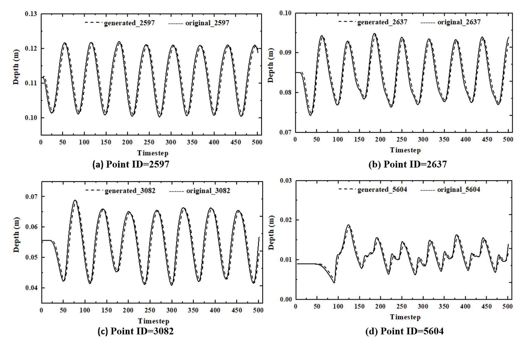
As shown in Fig. 6, the temporal variation of water depth is demonstrated at four points (locations shown in Fig. 3). It can be observed that the curves of water depth from the DCGAN have a slight difference from that of the original high fidelity model. In addition, the arriving time lags at four points can be noticed. The arrival time of flooding at point ID = 5604 is at timestep 50, where it is the farthest from the coastal boundary among the four points.
To further estimate the performance of the DCGAN, the correlation coefficient and RMSE are further illustrated in Fig. 7. It is evident that the values of RMSE are between to while the correlation coefficients are above . These results demonstrate that the DCGAN performs very well and the predicted fluid fields are in good agreement with the true fluid fields.


6.2 Case 2: Wave peak variation
In this case, the numerical illustration of the DCGAN was set up with a series of waves where the wave height varies. For a given input , Fig. 8 shows the comparison of predictive results between the DCGAN and the original high fidelity model. It is observed that most of water depth features are captured compared to the original fluid fields. In addition, the correlation coefficient of results at timesteps achieves values beyond shown in Fig. 9. These results highlight the good performances of the DCGAN in predictive analysis of fluid fields.
The temporal variations of water depth at four points are presented as the box plots in Fig. 10. The middle line represents the mean value , the upper represents the maximum (1 box) and the lower line denotes the minimum (-1 box). As regards to the mean value, the differences of mean values are less than at points ID = 2597, 2637, 3082 and 5604. The depth peak predicted by the DCGAN is at the point ID = 2597, which is comparable to that () from the original high fidelity model. A good performance of the DCGAN in predicting depth peak is achieved at points ID = 2637, 3082, and 5604. As for the minimum depth at the four points, the differences are less than as depicted in Fig. 10.
The error analysis of water depth solutions has been further carried out using the correlation coefficient and RMSE during the simulation period, as shown in Fig. 11. The values of RMSE fluctuate at different timesteps and are less than . The correlation coefficient of results between the DCGAN and the high fidelity model exceeds .


6.3 Computational efficiency
The DCGAN and the original high fidelity model were run on a computer (Intel Xeon(R) CPU@ 3.60GHz and a 449.5 GB memory). In terms of computation efficiency, it is worth mentioning that the online CPU cost used for running the DCGAN is less than , while for running the original high fidelity model. It can be seen that using the DCGAN, the CPU time is reduced by five orders of magnitude in comparison to the original high fidelity model.
To summarize, the DCGAN has successfully captured fluid flow features and provides the high-resolution fluid fields, especially for the nonlinear fluid flows in time and space. This serves as a technologically important motivation for using the DCGAN to efficiently forecast complicated fluid flows for realistic applications.
7 Conclusions
In this work, a DCGAN has been proposed for nonlinear spatio-temporal fluid flow prediction. It is the first time that the DCGAN is applied to prediction of spatially-temporally-coherent and high-dimensional nonlinear fluid flows. This novel DCGAN enables rapid and reliable prediction and can be used for providing risk reduction strategies in emergencies.
The performance of the DCGAN has been illustrated in the case of Hokkaido tsunami in this paper. Two study cases are set up with two series of waves with varying wave phase and wave height. To estimate the accuracy of the DCGAN, a comparison of nonlinear flow results obtained by the DCGAN and the original high fidelity model has been carried out. It is shown that the DCGAN is able to capture the complex flow features and exhibits an overall good agreement with the original high fidelity model. Error analysis has also been performed for further evaluation of the DCGAN through RMSE and correlation coefficient. In comparison to the original high fidelity model, the DCGAN achieves a reasonable accuracy in the whole simulation, while the online CPU cost is reduced by five orders of magnitude.
Overall, a general DCGAN for spatio-temporal fluid flow modelling is presented in this paper. It will be highly promising to apply the above DCGAN to various modelling problems, for example, turbulence modelling, ocean modelling, air pollution, and urban flows. Future work will focus on optimization of uncertainties in models and explore a hybrid machine learning approach (auto-encoder and GAN) for improving the accuracy and efficiency in prediction for complex problems. In this work we focus on the simulation of spatio-temporal distribution during a fixed simulation period for given varied boundary conditions, where the training and validation simulation periods are the same. In future, we will also focus on the real-time forecast– using the DCGAN for the lead-time prediction of spatio-temporal fluid flows. In addition, for realistic applications, a large number of snapshots (historical datasets), over a long time period, are needed for model training. The Classical Multidimensional Scaling (CMDS) proposed by (Kaiser et al., 2014, 2017) can be an efficient method to address this compression issue, which is able to convert a large set of observations into a set of low-dimensional states for visualization. Our future work will further explore the use of other compression methods (e.g. CMDS) along with the GAN to handle high dimensional data for real-time prediction in realistic applications.
Acknowledgments
The Authors acknowledge the support of: China Scholarship Council (No. 201806270238), funding from the EPSRC (MAGIC (EP/N010221/1), INHALE (EP/T003189/1), MUFFINS (EP/P033148/1) and PREMIERE (EP/T000414/1)), and the Royal Society (IEC/ NSFC/170563) in the UK.
References
- Brunton et al. (2019) Brunton SL, Noack B, Koumoutsakos P. Machine learning for fluid mechanics. ArXiv 2019;abs/1905.11075.
- Chang and Tsai (2016) Chang FJ, Tsai MJ. A nonlinear spatio-temporal lumping of radar rainfall for modeling multi-step-ahead inflow forecasts by data-driven techniques. Journal of Hydrology 2016;535:256–69.
- Creswell et al. (2018) Creswell A, White T, Dumoulin V, Arulkumaran K, Sengupta B, Bharath AA. Generative adversarial networks: An overview. IEEE Signal Processing Magazine 2018;35(1):53–65.
- Fang et al. (2013) Fang F, Pain CC, Navon I, Elsheikh A, Du J, Xiao D. Non-linear petrov–galerkin methods for reduced order hyperbolic equations and discontinuous finite element methods. Journal of Computational Physics 2013;234:540–59.
- Fang et al. (2014) Fang F, Zhang T, Pavlidis D, Pain C, Buchan A, Navon I. Reduced order modelling of an unstructured mesh air pollution model and application in 2d/3d urban street canyons. Atmospheric Environment 2014;96:96–106.
- Farimani et al. (2017) Farimani AB, Gomes J, Pande VS. Deep learning the physics of transport phenomena. arXiv preprint arXiv:170902432 2017;.
- Geneva and Zabaras (2019) Geneva N, Zabaras N. Quantifying model form uncertainty in reynolds-averaged turbulence models with bayesian deep neural networks. Journal of Computational Physics 2019;.
- Gonzalez and Balajewicz (2018) Gonzalez FJ, Balajewicz M. Learning low-dimensional feature dynamics using deep convolutional recurrent autoencoders. arXiv preprint arXiv:180801346 2018;.
- Goodfellow (2016) Goodfellow I. Nips 2016 tutorial: Generative adversarial networks. arXiv preprint arXiv:170100160 2016;.
- Goodfellow et al. (2014) Goodfellow I, Pouget-Abadie J, Mirza M, Xu B, Warde-Farley D, Ozair S, Courville A, Bengio Y. Generative adversarial nets. In: Advances in neural information processing systems. 2014. p. 2672–80.
- Hu et al. (2019a) Hu R, Fang F, Pain C, Navon I. Rapid spatio-temporal flood prediction and uncertainty quantification using a deep learning method. Journal of Hydrology 2019a;.
- Hu et al. (2018) Hu R, Fang F, Salinas P, Pain C. Unstructured mesh adaptivity for urban flooding modelling. Journal of hydrology 2018;560:354–63.
- Hu et al. (2019b) Hu R, Fang F, Salinas P, Pain C, Domingo NS, Mark O. Numerical simulation of floods from multiple sources using an adaptive anisotropic unstructured mesh method. Advances in Water Resources 2019b;123:173–88.
- Isola et al. (2017) Isola P, Zhu JY, Zhou T, Efros AA. Image-to-image translation with conditional adversarial networks. In: Proceedings of the IEEE conference on computer vision and pattern recognition. 2017. p. 1125–34.
- Kaiser et al. (2017) Kaiser E, Li R, Noack BR. On the control landscape topology. In: The 20th World Congress of the International Federation of Automatic Control (IFAC). 2017. p. 1–5.
- Kaiser et al. (2014) Kaiser E, Noack BR, Cordier L, Spohn A, Segond M, Abel M, Daviller G, Östh J, Krajnović S, Niven RK. Cluster-based reduced-order modelling of a mixing layer. Journal of Fluid Mechanics 2014;754:365–414.
- Kalteh (2013) Kalteh AM. Monthly river flow forecasting using artificial neural network and support vector regression models coupled with wavelet transform. Computers & Geosciences 2013;54:1–8.
- Kasiviswanathan et al. (2016) Kasiviswanathan K, He J, Sudheer K, Tay JH. Potential application of wavelet neural network ensemble to forecast streamflow for flood management. Journal of hydrology 2016;536:161–73.
- Kisi et al. (2012) Kisi O, Shiri J, Nikoofar B. Forecasting daily lake levels using artificial intelligence approaches. Computers & Geosciences 2012;41:169–80.
- Laloy et al. (2017) Laloy E, Hérault R, Jacques D, Linde N. Efficient training-image based geostatistical simulation and inversion using a spatial generative adversarial neural network. arXiv preprint arXiv:170804975 2017;.
- Ledig et al. (2017) Ledig C, Theis L, Huszár F, Caballero J, Cunningham A, Acosta A, Aitken A, Tejani A, Totz J, Wang Z, et al. Photo-realistic single image super-resolution using a generative adversarial network. In: Proceedings of the IEEE conference on computer vision and pattern recognition. 2017. p. 4681–90.
- Li and Wand (2016) Li C, Wand M. Precomputed real-time texture synthesis with markovian generative adversarial networks. In: European Conference on Computer Vision. Springer; 2016. p. 702–16.
- Lohani et al. (2014) Lohani AK, Goel N, Bhatia K. Improving real time flood forecasting using fuzzy inference system. Journal of hydrology 2014;509:25–41.
- Miyanawala and Jaiman (2017) Miyanawala TP, Jaiman RK. An efficient deep learning technique for the navier-stokes equations: Application to unsteady wake flow dynamics. arXiv preprint arXiv:171009099 2017;.
- Nair et al. (2019) Nair AG, Yeh CA, Kaiser E, Noack BR, Brunton SL, Taira K. Cluster-based feedback control of turbulent post-stall separated flows. Journal of Fluid Mechanics 2019;875:345–75.
- Östh et al. (2015) Östh J, Kaiser E, Krajnović S, Noack BR. Cluster-based reduced-order modelling of the flow in the wake of a high speed train. Journal of Wind Engineering and Industrial Aerodynamics 2015;145:327–38.
- Pain et al. (2001) Pain C, Umpleby A, De Oliveira C, Goddard A. Tetrahedral mesh optimisation and adaptivity for steady-state and transient finite element calculations. Computer Methods in Applied Mechanics and Engineering 2001;190(29-30):3771–96.
- Prakash et al. (2014) Prakash O, Sudheer K, Srinivasan K. Improved higher lead time river flow forecasts using sequential neural network with error updating. Journal of Hydrology and Hydromechanics 2014;62(1):60–74.
- Radford et al. (2015) Radford A, Metz L, Chintala S. Unsupervised representation learning with deep convolutional generative adversarial networks. arXiv preprint arXiv:151106434 2015;.
- Reed et al. (2016) Reed S, Akata Z, Yan X, Logeswaran L, Schiele B, Lee H. Generative adversarial text to image synthesis. arXiv preprint arXiv:160505396 2016;.
- Reichstein et al. (2019) Reichstein M, Camps-Valls G, Stevens B, Jung M, Denzler J, Carvalhais N, et al. Deep learning and process understanding for data-driven earth system science. Nature 2019;566(7743):195.
- Ströfer et al. (2018) Ströfer CM, Wu J, Xiao H, Paterson E. Data-driven, physics-based feature extraction from fluid flow fields. arXiv preprint arXiv:180200775 2018;.
- Wang et al. (2018) Wang Z, Xiao D, Fang F, Govindan R, Pain CC, Guo Y. Model identification of reduced order fluid dynamics systems using deep learning. International Journal for Numerical Methods in Fluids 2018;86(4):255–68.
- Xiao et al. (2019) Xiao D, Fang F, Zheng J, Pain C, Navon I. Machine learning-based rapid response tools for regional air pollution modelling. Atmospheric Environment 2019;199:463–73.
- Xiao et al. (2016) Xiao D, et al. Non-intrusive reduced order models and their applications. Ph.D. thesis; Imperial College London; 2016.
- Xie et al. (2018) Xie Y, Franz E, Chu M, Thuerey N. tempogan: A temporally coherent, volumetric gan for super-resolution fluid flow. ACM Transactions on Graphics (TOG) 2018;37(4):95.
- Yang et al. (2017) Yang T, Asanjan AA, Welles E, Gao X, Sorooshian S, Liu X. Developing reservoir monthly inflow forecasts using artificial intelligence and climate phenomenon information. Water Resources Research 2017;53(4):2786–812.