Data-driven design of explicit predictive controllers
using model-based priors
Abstract
In this paper, we propose a data-driven approach to derive explicit predictive control laws, without requiring any intermediate identification step. The keystone of the presented strategy is the exploitation of available priors on the control law, coming from model-based analysis. Specifically, by leveraging on the knowledge that the optimal predictive controller is expressed as a piecewise affine (PWA) law, we directly optimize the parameters of such an analytical controller from data, instead of running an on-line optimization problem. As the proposed method allows us to automatically retrieve also a model of the closed-loop system, we show that we can apply model-based techniques to perform a stability check prior to the controller deployment. The effectiveness of the proposed strategy is assessed on two benchmark simulation examples, through which we also discuss the use of regularization and its combination with averaging techniques to handle the presence of noise.
keywords:
Data-driven control; learning-based control; predictive control; explicit predictive control, ,
1 Introduction
For its capability of handling constraints, Model predictive control (MPC) is a widely employed technique for advanced control applications (see, e.g., [24, 23, 19, 14, 21]). Due to the increasing complexity of the systems to be controlled, the model required by MPC is often no longer parameterized from the physics but learned from data in a black-box fashion. However, this identification step generally takes the lion’s share of the time and effort required for control design. In the last years, research has thus benched into two main direction. On the one side, efforts has been focused on improving and easing learning procedures [9, 20]. On the other side, many approaches have been proposed to directly employ data for the design of predictive controllers, while bypassing any model identification step. Among existing works in this direction, we recall the foundational contributions of [10, 5], which have been extended to handle tracking problems [4], to deal with nonlinear systems [6], and to improve the performance in the presence of noise [13, 11], just to mention a few. For both traditional and data-driven predictive controls, the computational effort required to solve the related constrained optimization problem is known to be a potential limit for its application, especially for fast-sampling systems. Nonetheless, when the MPC problem is relatively small, i.e., one has to control a low order system and/or the prediction horizon is relatively short, this limitation can be overcome by explicitly deriving its solution [3]. In fact, when the cost of the optimization problem is quadratic and the constraints are linear, the explicit solution of MPC is known to be a Piece-Wise Affine (PWA) state feedback law.
In this work, we propose an approach to directly learn explicit predictive control laws from data. More specifically, we initially build on the foundational results in [12, 26] and on model-based priors (namely, the aforementioned fact that the optimal solution of linear MPC is PWA [3]), to construct a data-driven, multi-step closed-loop predictor. The latter is exploited to construct a fully data-based optimization problem, yielding the estimation of the parameters of the optimal predictive control law. As a by-product, we obtain a data-driven description of the closed-loop behavior, which can be used in combination with existing model-based techniques (see, e.g., [22]) to check the stability of the system controlled with the data-driven explicit controller, prior to its deployment. As far as we are aware, this is the first time a data-driven predictive control strategy is provided together with a preliminary assessment of its closed-loop performance.
We should mention here that an early attempt to obtain a data-driven counterpart of explicit MPC was already carried out in [25]. However, the strategy proposed therein relies on an implicit open-loop identification step. Another method was presented in [8], by relying on the behavioral predictor used in [11, 5]. Even though that method involves no open-loop identification phase and it does not require the state to be fully measurable, the latter does not leverage on priors coming from model-based analysis and design. Nonetheless, by leveraging on priors, we are here able to retrieve a data-based characterization of the closed-loop and, thus, practically assess its stability in a data-driven fashion prior to its deployment. This is instead not possible in [8], where stability cannot be directly assessed nor it is theoretically guaranteed in presence of noisy data.
The remainder of the paper is organized as follows. The targeted problem is formalized in Section 2, while all the steps required to obtain its data-driven formulation from priors are introduced in Section 3. The explicit control law is derived in Section 4, where we additional discuss practical aspects for its implementation, certified deployment and noise handling. The effectiveness of the proposed strategy is assessed on two benchmark examples in Section 5. Section 6 concludes the work and indicates some directions for future research.
Notation
We denote with the set of natural numbers, that includes zero. Let , and be the set of real numbers, column vectors of dimension and dimensional real matrices, respectively. Given , its transpose is , its Moore-Penrose inverse is and, when its inverse is indicated as . Given a vector , indicates its rows from to , with . For a matrix , denotes a sub-matrix comprising the first rows and columns of , with and . Identity matrices are denotes as , while zero matrices and vectors will be denoted as . If a matrix is positive definite (positive semi-definite), this is denoted as (). Given a vector , the quadratic form is compactly indicated as . Given a signal and , we denote with the associated Hankel matrix
| (1) |
while, for , we introduce
| (2) |
2 Problem formulation
Consider the class of discrete-time linear, time invariant (LTI), controllable systems with fully measurable state, i.e.,
| (3) |
where denotes the state of at time , is an exogenous input and is the associated noiseless output. Let us consider the following model predictive control (MPC) problem:
| (4a) | |||
| (4b) | |||
| (4c) | |||
| (4d) | |||
The objective of (4) is to steer both the (predicted) state and the input to zero, over a prediction horizon of prefixed length . Optimality is indeed dictated by: the distance of the predicted state from zero, penalized with over the whole horizon except for the terminal state (weighted via ), and the control effort, penalized via . Meanwhile, a set of polyhedral constraints dictated by (4c) has to be satisfied, with , and , while relying on the latest information on the system (see (4d)). Assume also that the matrices and characterizing the dynamics of are unknown, and that we can access a set of input/output data pairs , where and denote the available input and output sequences, respectively, satisfying the following assumptions.
Assumption 1 (Persistently exciting inputs).
The input sequence is persistently exciting of order .
Assumption 2 (Noisy outputs).
The output sequence is corrupted by noise, namely
| (5) |
where is the realization of a zero mean white noise with covariance .
Assumption 3 (Sufficiently long dataset).
The length of the dataset satisfies the following:
3 Exploiting priors for explicit DDPC
To attain our goal, it is fundamental to replace the model in (4b) with an expression that directly depends on the available data, by also not forgetting what we have learned from model-based predictive control. To start with, we thus recall the following lemma, explicitly stating the form of the optimal explicit predictive controller in our setting [3].
Lemma 1 (On the solution of (4)).
Let denote the vector stacking the inputs over the prediction horizon, i.e.,
| (6) |
The optimal control sequence solving (4) is a continuous piecewise affine (PWA) function of .
Then, we generalize the one-step ahead predictor introduced in [12] to the multi-step case. To this end, it is important to recall that, thanks to Assumptions 1, 3 and the Fundamental Lemma [26], the following rank condition holds:
| (7) |
We can now derive the multi-step data-based predictor as follows.
Theorem 1 (Data-based multi-step predictor).
Proof.
The proof follows the steps of the one in [12, Appendix B]. Specifically, let and be respectively defined as:
with being full row rank, i.e., . By the Rouché-Capelli theorem, for any given , the equality
admits infinite solutions of the form
| (9) |
with being the orthogonal projector onto the kernel of . Meanwhile, based on the model in (4b), the predicted state sequence can be defined as a function of and as:
| (10) |
In turn, such a sequence can be recast as a function of , i.e.,
where the second equality straightforwardly follows from (10) and the definition of . By replacing with (9), we then obtain
as , based on the definition of the projector. ∎
This preliminary result allows us to exploit priors on the solution of (4) for the definition of the DDPC problem. In fact, according to Lemma 1, we can parameterize the control sequence as:
| (11) |
where and are the (unknown) feedback and affine gains characterizing the control law, dictates the associated polyhedral partition, for , and the amounts of modes is dictated by the number of possible combinations of active constraints. Therefore, for a given state , the input sequence is the affine function
| (12) |
with and denoting the gains associated to the active control law, and with
Based on this parameterization, we can compute a data-based closed-loop characterization of the predictor in (4b), as outlined in the following theorem.
Theorem 2 (Closed-loop multi-step predictor).
Proof.
For the Rouché-Capelli theorem, there exists an matrix and a -dimensional vector such that (13b)-(13c) hold. Meanwhile, replacing (12) into the open-loop predictor in (8), the predicted state sequence can be represented as:
By combining these two results, the closed-loop representation in (13) and the equivalent definition of the input sequence in (14) straightforwardly follow. ∎
By leveraging on (13)-(14), we can now equivalently recast the predictive control task in (4) as an optimization problem with the closed-loop matrices being the decision variables, as follows111Notice that the term in the cost that depends only on has been neglected. This can be done without loss of generality, as the optimal solution does not change.:
| (15a) | |||
| (15b) | |||
| (15c) | |||
| (15d) | |||
| (15e) | |||
| (15f) | |||
In (15), , , and
Note that, the last constraints (see (15e)-(15f)) are introduced for the problem to be consistent with the closed-loop representation in (13).
This shift from an open-loop predictor to its closed-loop counterpart allows us to directly learn the control law from data, and avoid any system identification step.
4 Learning Explicit DDPC
To derive its explicit solution, the problem in (15) is manipulated to obtain a multi-parametric Quadratic Program (mp-QP). As a preliminary step, we condense the unknowns of (15) into a single variable:
| (16) |
Accordingly, we can recast (15) as the following mp-QP
| (17a) | |||
| (17b) | |||
| (17c) | |||
where
| (18a) | ||||
| (18b) | ||||
| (18c) | ||||
| and | ||||
By focusing on in (17a), it can be proven that this weighting matrix satisfies the following lemma.
As the cost should be strictly convex for a unique explicit solution to be retrieved, this feature of prevents us from deriving the explicit law. To overcome this limitation, we introduce a regularization term in the cost of (17), thus replacing the weight with:
| (19) |
where is an hyper-parameter to be tuned222The cost has been normalized to ease the subsequent derivations.. The data-driven control problem then corresponds to the regularized mp-QP:
| (20a) | |||
| (20b) | |||
| (20c) | |||
4.1 Derivation of the explicit DDPC law
The introduction of the regularizer in (20) allows us to derive the explicit DDPC law through the manipulation of the Karush-Kuhn-Tucker (KKT) conditions associated with the new DDPC problem. To ease the computations, let us consider the following further assumption.
Assumption 4 (Non-degenerate constraints).
The active constraints of (20) are linearly independent.
Based on this assumption, we now follow the same steps used to derive the explicit model-based predictive control law in [3].
The KKT conditions for the regularized DDPC problem in (20) are:
| (21a) | |||
| (21b) | |||
| (21c) | |||
| (21d) | |||
| (21e) | |||
| where and are the Lagrange multipliers associated with inequality and equality constraints in (20b) and (20c), respectively. | |||
Let us focus on the -th set of active constraints only, distinguishing between the Lagrange multipliers associated with a given active and inactive inequality constraints. We respectively denote them as and . It is straightforward to notice that the combination of (21b) and (21c) leads to the following condition on :
By merging (21b) and (21e) for the -th set of active constraints, it is also straightforward to show that the optimal solution satisfies
| (22) |
where
and , and are the rows of , and coupled with the considered set active constraints. By leveraging on (21a), we can now express our optimization variable as a function of the Lagrange multipliers, i.e.,
| (23) |
where
We can now replace the latter into (22) to obtain an explicit expression of the Lagrange multipliers as functions of the matrices characterizing (20):
| (24) |
In turn, this allows us to explicitly retrieve as:
| (25) |
and the associated optimal input sequence as
| (26) |
Thus, the input to be fed to the system when the -th set of constraints is active is defined as:
| (27) |
Through (21c) and (21d), we can finally define the polyhedral region associated with the considered combination of active constraints, which is dictated by the following inequalities:
| (28a) | |||
| (28b) | |||
The complete data-driven expression for (11) is then straightforwardly obtained by following the above steps for all possible combinations of the active constraints. This operation ultimately yields an optimal input sequence of the form:
| (29) |
where is given by the number of possible combinations of active constraints, corresponds to (26), for all , while can be easily obtained from (28). Consequently, the input to be fed to starting from can be retrieved by evaluating the PWA law
| (30) |
with given by (27), for .
Remark 2 (On Assumption 4).
Although introduced to ease computations, we remark that Assumption LABEL:ass:non_degenrate is not restrictive. Indeed, degenerate cases can be straightforwardly handled via existing approaches, e.g., see [3].
Remark 3 (Data-driven and model-based).
Within a noiseless setting, the results in Theorem 2 and the one-to-one correspondence between the chosen parameterization of the control law in (11) and its model-based counterpart guarantee the equivalence between (4) and (15). Therefore, when there is no noise, the data-driven explicit controller coincides with the E-MPC law as .
4.2 Implementing Explicit DDPC
Based on the available batch of data and the features of the considered predictive control problem, the explicit DDPC law can be completely retrieved offline from the available measurements, as summarized in Algorithm 1.
Input: Dataset ; penalties ; ; horizon ; constraint matrices ; regularization parameter .
-
1.
Construct the data-based matrices , , .
-
2.
Build , , , in (18a) based on the cost and constraints of the DDPC problem.
-
3.
Find all possible combinations of active constraints.
-
4.
For each combination, isolate the matrices , and characterizing (22)
-
5.
If not all rows of are linearly independent, handle the degeneracy, e.g., as in [3].
- 6.
-
7.
Merge polyhedral regions as in [2].
-
8.
Extract the first component of the optimal input sequence .
Output: Optimal input .
Given the data, one has to initially construct the Hankel matrices needed to build the DDPC problem (see steps 0.-0.). Once all the possible combinations of active constraints have been detected at step 0. and degenerate scenarios have been handled (see step 0.), at step 0. the local controllers and the associated polyhedral regions are retrieved according to (26)-(28). Lastly, at step 0., the optimal control sequence is simplified, by merging polyhedral regions whenever possible. After this step, the explicit optimal input can simply be retrieved by extracting the first element of the input sequence (see step 0.).
Once the explicit DDPC law has been retrieved, the computation of the optimal input at each time instant simply consists of a function evaluation. Specifically, one has to search for the polyhedral region the current state belongs to, and apply the corresponding parametric law. We stress that this computational advantage is retained for simple control problems only (i.e., for short prediction horizon and small systems). Indeed, the complexity of the PWA law is known to rapidly increase [7] with the one of the DDPC problem to be solved, analogously to the model-based case.
4.3 Explicit data-driven predictive control and closed-loop stability
When designing a controller in a data-driven setting, it is crucial to check the stability of the resulting closed-loop system before the controller deployment. Towards this objective, we now show how the peculiar features of the explicit data-driven predictive control can be leveraged in combination with existing techniques to devise an off-line, data-driven stability test. To this end, let us assume that the -th set of constraints is active and consider the following multi-step ahead closed-loop model:
| (31) |
obtained by combining (13) with the result of our explicit derivation in (25), where stacks the state predicted by the learned closed-loop model, i.e.,
From (31), we can then isolate the learned one-step ahead closed-loop model, namely
| (32a) | |||
| where | |||
| (32b) | |||
| (32c) | |||
When performed for each mode , these manipulations allow us to retrieve the data-driven closed-loop transition matrix for each . Retrieving these matrices ultimately enables us to apply model-based techniques, e.g., the ones presented in [22], to shed a light on the features of the final closed-loop. As an example, one can search for a matrix satisfying the following sufficient conditions for asymptotic stability:
| (33a) | |||
| (33b) | |||
or, alternatively, look for the set of matrices verifying the following LMIs:
| (34a) | |||
| (34b) | |||
| which are also sufficient conditions for asymptotic stability. | |||
Remark 4 (On the tuning of in (4a)).
When is known to be open-loop stable, the terminal weight in (4a) is generally selected as the solution of the Lyapunov equation
This equation can be directly translated into its data-driven counterpart by exploiting [12] as follows:
| (35) |
with
thus providing a data-based approach for the selection of this parameter.
Remark 5 (Hyper-parameter tuning).
The possibility of performing an off-line data-based stability check on the data-driven explicit law can be useful to preliminarily assess the effects of different choices of the tuning parameters , and in (4a) and in (19), allowing one to discard the ones resulting in a failure of the data-driven stability tests.
4.4 Regularization and noise handling
As highlighted in Remark 1, all the equivalences we rely on to derive the explicit predictive control law are verified when is noiseless. However, in practice, in Assumption 2 is generally a non-zero matrix.
To cope with noisy data, we follow the footsteps of [5, 13] and propose to leverage on the regularization term introduced in (19). Indeed, as in standard ridge regression [18], this additional element of the cost steers all the components of towards small values. In turn, this potentially limits the impact of noise on the constraints in (20b)-(20c) and, thus, on the final explicit law. This shrinkage effect is modulated by the regularization parameter , with the reduction in the magnitude of being stronger whenever large values of are considered. At the same time, implicitly changes the balance between the penalties in the original data-driven control problem in (15), with excessively high values of potentially driving the explicit data-driven controller far away from its model-based counterpart. The choice of this hyper-parameters thus becomes an important tuning-knob of the approach, requiring one to trade-off between handling noise and keeping explicit DDPC as close as possible to the implicit DDPC problem.
Although the stability checks in (33)-(34) can be used to have a preliminary assessment on the effect of different choices of , at the moment this balance can only be attained through closed-loop trials for several values of . Such a procedure allows one to ultimately select the hyper-parameter that best fits one’s needs, at the price of requiring closed-loop experiments that can be rather safety-critical in practice, especially when a simulator of the system is not available.
Whenever multiple experiments can be performed by feeding the plant with the same input sequence , the burden associated to the choice of can be alleviated by exploiting the features of Assumption 2 itself. In this scenario, one can indeed replace with the averaged dataset , where and
| (36) |
with denoting the output of the -th experiment. Since the noise is assumed to be zero mean, the law of large numbers asymptotically yields
| (37) |
As such, when the number of experiments increases, the role of in handling noise is progressively less dominant. In this case, should then be used only to make the DDPC problem well-defined. Any small is acceptable for this purpose.
5 Numerical examples
The performance of the explicit predictive controller are now assessed on two benchmark examples: the regulation to zero of the stable open-loop system of [3], for the case when the state is fully measurable; and the altitude control of a quadcopter. Since the last example features an open-loop unstable linearized plant, data are collected in closed-loop, by assuming that the drone is stabilized by an (unknown) pre-existing controller. In both the examples, the level of noise acting on the measured states is assessed through the averaged Signal-to-Noise-Ratio (SNR):
| (38) |
where and denote the -th components of the state and the measurement noise, respectively. All computations are carried out on an Intel Core i7-7700HQ processor, running MATLAB 2019b.
5.1 Open-loop stable benchmark system
Let us consider the benchmark system described by:
| (39) |
Our goal is to regulate both components of the state to zero, while enforcing the following box-constraint on the input:
| (40) |
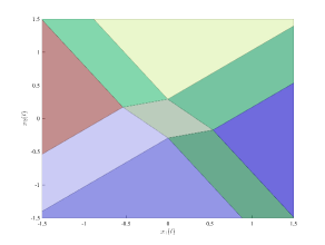
Towards this goal, we collect a set of input/state pairs, by feeding with an input sequence uniformly distributed within the interval . According to Assumption 2, the measured states are corrupted by an additive zero-mean white noise sequence, with variance yielding dB. The parameters characterizing the DDPC problem to be solved are selected as in [3], namely , , and is chosen as the solution of the data-driven Lyapunov in (35). By setting , the partition associated with the explicit data-driven predictive controller333The partition is plotted thanks to the Hybrid Toolbox [1]. is the one shown in Figure 1, which approximately correspond to that reported in [3]444The negligible differences with respect to the model-based partition are due to the noise on the batch data.. Prior to the controller deployment, we have performed the data-based closed-loop stability check in (33), resulting in555The LMIs in (33) are solved with CVX [17, 16].
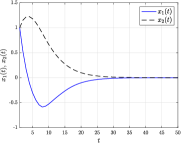
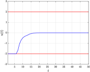
This indicates that the explicit law preserves the stability of the open-loop system. Figure 2 report the trajectories of the state and the optimal input obtained over a noise-free closed-loop tests with the explicit data-driven law, which confirm its effectiveness and validate the result of the data-driven stability check.
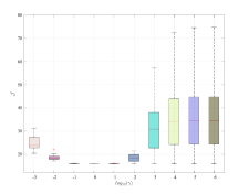
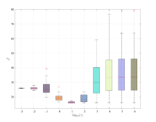
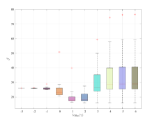
We now assess the sensitivity of the explicit controller to the choice of over Monte-Carlo realizations of the batch datasets , for different noise levels. This evaluation is performed by looking at the cost of the controller over the same noiseless closed-loop test of length considered previously, i.e.,
| (41) |
As shown in Figure 3, the value of that leads to the minimum closed-loop cost tends to decrease when the noise level increases, supporting our considerations in Section 4.4. At the same time, by properly selecting we attain a cost , which is generally close to the oracle , which is the one achieved by the oracle law, i.e., the model-based predictive controller obtained by exploiting the true model of . These results additionally show that, for increasing levels of noise, the choice of becomes more challenging, since the range of values leading to the minimum progressively shrinks. Note that, when is excessively small the optimal input is always zero and evolves freely666This behavior is also observed for , and when dB, dB and dB, respectively..
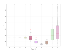
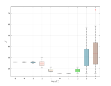
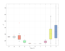
We additionally evaluate the effect of averaging, by looking at the performance index in (41) over Monte-Carlo data-collections for an increasing number of repeated experiments of length . The measurements are affected by noise, yielding dB. Figure 4 shows that the use of the averaged dataset has a similar effect to a reduction of the noise level. Indeed, for increasing the optimal slowly shifts towards smaller values, thus further implying the gradual reduction in the impact of on noise handling.
5.2 Altitude control of a quadcopter
As a final case study, we consider a nonlinear system, namely the problem of controlling the altitude of a quadcopter, to perform landing or take-off maneuvers. To this end, we exploit the same simulator used in [15] to collect the data and to carry out the closed-loop experiments with the learned explicit law. Let [m] be the altitude of the quadcopter, [m/s] be its vertical velocity and [deg] its roll, pitch and yaw angles at time . Both the the altitude [m] and the vertical velocity are assumed to be measured, with the measurement being corrupted by a zero-mean white noise, resulting in 30 dB over these two outputs. As this system is open-loop unstable, the data collection phase is carried out in closed-loop for [s] at a sampling rate of [Hz], by using the four proportional derivative (PD) controllers introduced in [15]. The altitude set point used at this stage is generated uniformly at random in the interval [m]. The set points for all the attitude angles are instead selected as slowly variable random signals within the interval [rad]. These choices yield a dataset of length , that satisfies Assumption 1 and allows us to retain information on possible non-zero angular configurations.
The three attitude controllers introduced in [15] are further retained in testing to keep the attitude angles at zero and to decouple the altitude dynamics from that of the other state variables. Within this setting, the explicit data-driven law is designed by imposing , , and . To mitigate the effect of the gravitational force, the design and closed-loop deployment of the designed explicit controller are carried out by pre-compensating it. As a result, the input to be optimized is
| (42) |
where [kg] is the mass of the quadcopter, [m/s] is the gravitational acceleration and is the input prior to the compensation. A similar approach is adopted for the control problem to fit our framework in both landing and take-off scenarios. We thus consider the reduced state
| (43) |
where [m] is the altitude set point. To avoid potential crashes of the quadcopter, in designing the explicit law we impose the following constraint on the state of the system:
| (44) |
which, in turn, guarantees the altitude to be always non-negative. Meanwhile, the pre-compensated input is constrained to the interval:
| (45) |
where the lower bound corresponds to a null input and the upper limit is dictated by the maximum power of the motors777The reader is referred to [15] for additional details on the system..
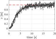
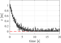
The performance of the learned explicit law attained in take-off and landing are reported in Figure 5. Here we consider closed-loop tests in which the altitude and the vertical velocity are noisy, with the noise acting on the closed-loop measurements sharing the features of that corrupting the batch ones. Despite the noise acting on the initial condition at each step, both maneuvers are successfully performed, thus showing the effectiveness of the retrieved explicit data-driven laws.
6 Conclusions
By leveraging on the known PWA nature of the explicit MPC law within linear quadratic predictive control, in this paper we propose an approach to derive such an explicit controller from data only, without undertaking a full modeling/identification step. Thanks to the formalization of the problem, well-known model-based techniques can be straightforwardly adapted to check the stability of the closed-loop system before deploying the controller.
Future research will be devoted to extend these preliminary results to cases in which the state is not fully measurable, to exploit priors to guarantee practical closed-loop stability by design. Future work will also be devoted to formalize the connections between the explicit solution proposed in this paper and the one introduced in [8], consequently providing a comparative analysis of the two approaches.
References
- [1] A. Bemporad. Hybrid Toolbox - User’s Guide, 2004. http://cse.lab.imtlucca.it/~bemporad/hybrid/toolbox.
- [2] A. Bemporad, K. Fukuda, and F.D. Torrisi. Convexity recognition of the union of polyhedra. Computational Geometry, 18(3):141–154, 2001.
- [3] A. Bemporad, M. Morari, V. Dua, and E.N. Pistikopoulos. The explicit linear quadratic regulator for constrained systems. Automatica, 38(1):3–20, 2002.
- [4] J. Berberich, J. Köhler, M.A. Müller, and F. Allgöwer. Data-driven tracking MPC for changing setpoints. IFAC-PapersOnLine, 53(2):6923–6930, 2020. 21th IFAC World Congress.
- [5] J. Berberich, J. Köhler, M.A. Müller, and F. Allgöwer. Data-driven model predictive control with stability and robustness guarantees. IEEE Transactions on Automatic Control, 66(4):1702–1717, 2021.
- [6] J. Berberich, J. Köhler, M.A. Müller, and F. Allgöwer. Linear tracking MPC for nonlinear systems part II: The data-driven case. In arXiv/2105.08567, 2021.
- [7] F. Borrelli, M. Baotić, J. Pekar, and G. Stewart. On the complexity of explicit mpc laws. In 2009 European Control Conference (ECC), pages 2408–2413, 2009.
- [8] V. Breschi, A. Sassella, and S. Formentin. On the design of regularized explicit predictive controllers from input-output data. In arXiv/2110.11808, 2021.
- [9] A. Chiuso and G. Pillonetto. System identification: A machine learning perspective. Annual Review of Control, Robotics, and Autonomous Systems, 2(1):281–304, 2019.
- [10] J. Coulson, J. Lygeros, and F. Dörfler. Data-enabled predictive control: In the shallows of the DeePC. In 2019 18th European Control Conference (ECC), pages 307–312, 2019.
- [11] J. Coulson, J. Lygeros, and F. Dörfler. Regularized and distributionally robust data-enabled predictive control. In 2019 IEEE 58th Conference on Decision and Control (CDC), pages 2696–2701, 2019.
- [12] C. De Persis and P. Tesi. Formulas for data-driven control: Stabilization, optimality, and robustness. IEEE Transactions on Automatic Control, 65(3):909–924, 2019.
- [13] F. Dörfler, J. Coulson, and I. Markovsky. Bridging direct & indirect data-driven control formulations via regularizations and relaxations. In arXiv/2101.01273, 2021.
- [14] T. Faulwasser, M.A. Müller, and K. Worthmann. Recent advances in model predictive control: Theory, algorithms, and applications. 2021.
- [15] S. Formentin and M. Lovera. Flatness-based control of a quadrotor helicopter via feedforward linearization. In 2011 50th IEEE Conference on Decision and Control and European Control Conference, pages 6171–6176, 2011.
- [16] M. Grant and S. Boyd. Graph implementations for nonsmooth convex programs. In V. Blondel, S. Boyd, and H. Kimura, editors, Recent Advances in Learning and Control, Lecture Notes in Control and Information Sciences, pages 95–110. Springer-Verlag Limited, 2008. http://stanford.edu/~boyd/graph_dcp.html.
- [17] M. Grant and S. Boyd. CVX: Matlab software for disciplined convex programming, version 2.1. http://cvxr.com/cvx, March 2014.
- [18] T. Hastie, R. Tibshirani, and J.H. Friedman. The Elements of Statistical Learning: Data Mining, Inference, and Prediction. Springer series in statistics. Springer, 2009.
- [19] D. Hrovat, S. Di Cairano, H.E. Tseng, and I.V. Kolmanovsky. The development of model predictive control in automotive industry: A survey. In 2012 IEEE International Conference on Control Applications, pages 295–302, 2012.
- [20] L. Ljung. Perspectives on system identification. Annual Reviews in Control, 34(1):1–12, 2010.
- [21] D.Q. Mayne. Model predictive control: Recent developments and future promise. Automatica, 50(12):2967–2986, 2014.
- [22] D. Mignone, G. Ferrari-Trecate, and M. Morari. Stability and stabilization of piecewise affine and hybrid systems: an lmi approach. In Proceedings of the 39th IEEE Conference on Decision and Control (Cat. No.00CH37187), volume 1, pages 504–509 vol.1, 2000.
- [23] S.J. Qin and T.A. Badgwell. A survey of industrial model predictive control technology. Control Engineering Practice, 11(7):733–764, 2003.
- [24] J.B. Rawlings. Tutorial overview of model predictive control. IEEE control systems magazine, 20(3):38–52, 2000.
- [25] A. Sassella, V. Breschi, and S. Formentin. Learning explicit predictive controllers: theory and applications. In arXiv/2108.08412, 2021.
- [26] J.C. Willems, P. Rapisarda, I. Markovsky, and B.L.M. De Moor. A note on persistency of excitation. Systems & Control Letters, 54(4):325–329, 2005.