Data-driven control of nonlinear systems from input-output data*
Abstract
The design of controllers from data for nonlinear systems is a challenging problem. In a recent paper, De Persis, Rotulo and Tesi, “Learning controllers from data via approximate nonlinearity cancellation,” IEEE Transactions on Automatic Control, 2023, a method to learn controllers that make the closed-loop system stable and dominantly linear was proposed. The approach leads to a simple solution based on data-dependent semidefinite programs. The method uses input-state measurements as data, while in a realistic setup it is more likely that only input-output measurements are available. In this note we report how the design principle of the above mentioned paper can be adjusted to deal with input-output data and obtain dynamic output feedback controllers in a favourable setting.
I INTRODUCTION
Learning controllers from data is of uttermost importance and a fascinating topic, with foundations in both control theory and data science. Several recent approaches have been proposed for data-driven control, initially focusing, as is natural, on linear systems, e.g. [1, 2, 3, 4]. For nonlinear systems, some results have appeared as well, mostly focusing on special classes of nonlinear systems, bilinear [5, 6], polynomial [7, 8, 9], rational [10] or with quadratic nonlinearities [11], [12]. Other approaches consist of approximating general nonlinear control systems to classes for which data-driven design is possible [13, 14] or expressing nonlinear systems via a dictionary of known functions, in which case the design can aim at making the closed-loop system dominantly linear [15] or prescribing a desired output signal [16].
The understanding of the topic is far from having reached a mature phase, even in the case full measurements of the state are available. Yet, it can be argued that the use of these data-dependent design schemes in practice very much rely on the possibility that they work with output measurements data only, which dispenses the designer from requiring to know the state of the system – a very restrictive prior in many cases. In this paper we report on some early results on using data-driven control techniques in conjunction with input/output data for discrete-time nonlinear systems.
Related work. Even when a model is known, output feedback control for nonlinear systems is a challenging open problem [17, Section 8.7]. The certainty equivalence principle, which is valid for linear systems, is hard to extend to a nonlinear setting. Nonetheless, certain nonlinear discrete-time versions of the certainty equivalence principle have been obtained [18]. In [19], the state in a globally stabilizing state feedback (possibly generated by a finite horizon model predictive scheme) is replaced by an estimate provided by an observer under a uniform observability assumption to obtain a globally stabilizing output feedback controller.
The important uniform observability property [20, 21, 22] can be explored in different ways in the context of learning control from data. Since it guarantees the existence of an injective map from input/output sequences to the state, deep neural networks can be trained to approximate such a map and provide estimates of the state to be used in the given input-to-state stabilizing feedback, obtaining a locally asymptotically stable closed-loop system [23]. The injective map can also be used to define the regression relating the input/output sequences of the system and deep neural networks can be used to learn such a regression [24]. However, to the best of our knowledge there are very few other attempts at designing controllers for nonlinear system from input/output data.
Contribution. The aim of this note is to start the investigation of feedback design from input/output data for nonlinear discrete-time systems. We adopt the notion of uniform observability, which allows us to extend some of the design procedures introduced in [2]. Namely, we consider past inputs and outputs as fictitious state variables and obtain a form of the system for which the data-driven “state” feedback design techniques for nonlinear systems of [15] can be used. The implementation of the controller is then carried out by replacing the past input/output measurements with the quantities returned by a dead-beat observer of the output and a chain of integrators driven by the input. A formal analysis of the stability of the overall closed-loop system is then presented along with a discussion about the proposed solution.
In Section II we recall the notion of observability that we adopt for our analysis and introduce an auxiliary system that reproduces the input/output behaviour of the system to control. The auxiliary system is extended in Section III-A with a chain of integrators that provides the past inputs of the system to be used in the controller. The design of the output feedback dynamic controller based on input/output data is presented in Section III. The analysis of the closed-loop system to show the convergence of the system’s and the controller’s state to the origin is the topic of Section IV, along with a discussion of the result.
II Preliminaries
We consider the single-input single-output nonlinear discrete-time system
| (1) |
where , , and . are continuous functions of their arguments with domains and . These functions are unknown. The dimension of the state-space is not necessarily known.
II-A Dataset
A dataset consisting of open-loop input-output measurements
| (2) |
is available, where the positive integers will be specified later. The samples in the dataset are obtained from off-line experiment(s) conducted on system (1), hence they satisfy the equations (1), namely
For our purpose of designing an output feedback controller from it is not required that all the samples of the dataset are sequentially obtained in a single experiment. In fact, even multiple experiments collecting samples suffice. This is useful especially when dealing with unstable dynamics.
II-B Uniform Observability
The problem of interest is to design an output feedback controller that stabilizes the nonlinear system, based on the dataset . To this purpose, we need to infer the behavior of the state from input-output measurements, for which suitable “observability” conditions on the system (1) are required. Before stating them, we introduce some notation. We let
| (3) |
Note that (3) gives . To reduce the notational complexity, we introduce , which denotes the sequence of values . Hence, the last identity above is rewritten as . In what follows, we will use symbols like also to denote the vector .
The following is the main assumption on system (1).
Assumption 1
Let and be compact sets such that contains the origin of . There exists such that, for any , the mapping
| (4) |
is injective as a function of on .
Following [22, Definition 1], we refer to the assumption above as a uniform observability on property. It is observed in [22] that, if are continuously differentiable functions, uniform observability is not restrictive in the sense that a nonuniform distinguishability property and a nonuniform observability rank condition imply uniform observability. Since for any the mapping remains injective, we do not need to know the smallest for which Assumption 1 holds.
For any , the function
such that , is injective on and one can define a left inverse
such that for all .
II-C An auxiliary system
We introduce a system equivalent to (1) which is better suited for control design. By equivalent it is meant that the new system has the same input-output behavior of system (1) when properly initialized. We use this auxiliary system for control design purposes. Later on we show the effect of the designed controller on the actual system (1).
For any , define the functions
| (5) |
with the pair in the Brunovsky form. The domain of , is . Under the standing assumptions on , these functions are continuous and zero at .
In the result below, for a , we let be an input sequence applied to system (1) and its output response from some initial condition .
Lemma 1
Proof. For the sake of completeness, it is given in Appendix VI-A.
Example 1
We consider [15, Example 5]
| (7a) | |||
| (7b) | |||
with . We compute
which is globally invertible (Assumption 1 holds with .) with
Hence , where
| (8) |
From which, one computes
Hence the equivalent representation is given by
The original state is obtainable from the solution of the system above via the expression
where is as in (8). For this example and .
III Design of an output feedback controller from data
III-A A dynamic extension
System (6) is driven by the past samples of , which is the input to (1). These past values are obtained by adding a chain of integrators to the dynamics (6)
| (9) |
with the interconnection condition
which returns the system
| (10) |
Once the system’s state satisfies for some , the input-output behavior of this system matches the one of (1) for all . We will discuss later on the availability of such initial condition at a time .
III-B Control input design
To obtain that drives the chain of integrators making the dynamic controller, we argue as in [2, 15]. We first introduce the following:
Assumption 2
For any and any , where denotes the first entries of , it holds that , where is a vector of known continuous functions and is an unknown vector.
This is a technical assumption due to the need to give the nonlinearities of (10) a form for which the controller design is possible. Although it is restrictive, [15, Section VI.B] bypasses such an assumption by expressing as , where the term represents the nonlinearities that were excluded from , and then analyzing the stability of the system in the presence of the neglected nonlinearity . This analysis goes beyond the scope of this paper.
We consider the case in which the function comprises both a linear part and a nonlinear part , i.e.
The system (10) can then be written as
| (11) |
where
and the pair is in the Brunovsky canonical form.
III-C Data-dependent representation of the closed-loop system
Preliminary to the design of the controller is a data-dependent representation of the closed-loop system. We first introduce some notation. Recall the dataset in (2) and introduce, for ,
We assume that the samples of the dataset evolve in the domain of definition of (13).
Assumption 3
For any , and .
We let:
| (14) |
In the definition of , we are using the shorthand notation for . Under Assumption 3, bearing in mind the dynamics (11), the dataset-dependent matrices introduced in (14) satisfy
| (15) |
Remark 1
(Multiple experiments) This identity is obtained from the identities
We note that, for each , the identity does not require the quantities to be related to the corresponding quantities for . In other words, we could run -long independent experiments and collect the resulting input-output samples in
where denotes the number of the experiment, and are the input-output samples of the experiment . We could then redefine the matrices in (14) as
and the identity (15) would still apply.
We establish the following:
Lemma 2
Let the set of real-valued symmetric matrices of dimension be denoted by . This data-dependent representation leads to the following local stabilization result:
Proposition 1
Proof. Set . Then (18b), (18d) imply
which along with the definition of in (22), namely , implies (16). Hence, the data-dependent representation of system (13) given in Lemma 2 holds. By Schur complement, the constraint (18c) is equivalent to
Pre- and post-multiplying by and bearing in mind the definition of we obtain
which shows that is a Lyapunov function for the linear part of the closed-loop system. In particular note that the domain of definition of the function is the same as the one of system (23), hence, is defined at the origin. We have
In view of (19), in a neighborhood of the origin. This shows the claim.
III-D Region of Attraction
Proposition 1 provides a local stabilization result. Following [15], Proposition 1 can be extended to provide an estimate of the Region of Attraction (ROA) of the system (23). First we recall the following definitions.
Definition 1
[25, Definition 13.2] Suppose that is an asymptotically stable equilibrium for . Then the ROA of is given by
where is the solution to at time from the initial condition .
Definition 2
[25, Definition 13.4] A set is a positively invariant set for if for all , where .
Corollary 1
As the function is known from the data, the estimate of the ROA is computable.
IV Main result
To draw conclusions on the convergence of system (1), we first observe that the dynamical controller (20) uses its own state and the state to generate the control action . At time the state contains the past output measurements from the process (1), from which we only measure . To make the past measurements in available to the controller, we extend it with the dynamics
| (24) |
Then, for any and any , we have that for all , that is, independently of the initialization of (24), its state provides the vector of the past output measurements from time onward. Similarly, for any , system (20) is such that for all . See [19] for the same structure of the controller (20), (24).
Remark 2
System (24) is the so-called deadbeat observer, since for , the mapping would return . If both and a state-feedback stabilizer for system (1) were known, one could obtain a dynamic output feedback controller for the system (1). Here we are interested to the case in which this knowledge is not available and we design a dynamic output feedback controller under a suitable assumption on the nonlinearity (Assumption 2).
The following statement transfers the result obtained for the system (23) to the actual closed-loop system that includes the process (1).
Proposition 2
Let Assumptions 1, 2 and 3 hold. Consider the SDP (18), assume that it is feasible and let condition (19) hold. For any for which there exists such that , the solution of the system (1) in closed-loop with the time-varying controller comprised by (20), (24) and
| (25) |
that starts from , asymptotically converges to the origin.
Proof. First note that, by definition of the mapping and since and , each entry of is a continuous function of its arguments which is zero when these are zero, hence there exists a neighbourhood of the origin such that any point in the neighbourhood satisfies .
By definition of the mapping in Assumption 1 and (25), , where denotes the output response of the closed-loop system from the initial condition .
By the dynamics of the controller (20), (24), we have , for all and . Hence, by Lemma 1, the solution of (20), (24) are the same as those of system (23) intialized at . As , by Proposition 1 and Corollary 1, converges to the origin. By Lemma 1, for all , , which implies convergence of to the origin by continuity of .
The particular form of in (25) is due to the fact that, during the first -steps, the controller state does not provide an accurate value of the past input-output measurements of the system, hence the choice to apply an open-loop input sequence. After time steps, when such past measurements become available through the controller states , is set to the feedback .
We also remark that in the result above if the initial condition is sufficiently close to the origin and the initial sequence of control values does not drive the output response of (1) outside the set , then the designed controller (25) steers the state of the overall closed-loop system to the origin. Note that is known thanks to Corollary 1, hence the designer can check whether the initial control sequence and the corresponding measured output response are in . For the design of the initial control sequence, the designer could take advantage of some expert knowledge.
Remark 3
(Prior on input/output measurements) The controller is designed under the assumption that the input/output measurements collected during the experiment range over some specified sets – see Assumption 3 – where the measurements provide meaningful information about the system’s internal state. These sets are not known, hence, the feature that the evolution of the system during the experiments remains in the sets of interest must be considered as one of the priors under which the design is possible.
V Numerical example
We continue with Example 1 and consider the equations (7) with output . The system parameters are , and . The problem is to learn a controller for (7) from input-output data that renders the origin of the closed-loop system locally asymptotically stable.
We collect data by running , -long experiments with input uniformly distributed in and with an initial state in . For each experiment , we collect the samples . Then we construct data matrices , as detailed in Remark 1. The program (18) is feasible and we obtain the controller gain with
| (26) |
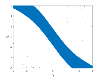
using the YALMIP toolbox [26], MOSEK solver [27]. To assess the effectiveness of the designed controller, instead of computing , which for this example provides a conservative estimate of the ROA, we depict in Fig. 1 the set of initial conditions for which, choosing for in (25), the state converges to zero. Note that the choice of is inessential. The set is obtained by letting the closed-loop system evolve for time steps and then checking whether or not the norm is smaller than on the interval .
VI CONCLUSIONS
We have examined a design of dynamic output feedback controllers for nonlinear systems from input/output data. The uniform observability property of the system, a prior in the approach, is instrumental to define a new set of coordinates, from which a data-driven “state”-feedback design can be conducted. The result is local and the size of the region of attraction is limited by the free evolution of the system during the first steps during which the dead-beat observer reconstructs the past input/output values that feed the controller. The design and analysis have been carried out in the favourable setting in which measurements are noise-free and the nonlinearities can be expressed via a dictionary of known functions. Regarding the future work, besides going beyond the favourable setting, we would like to explore either a more sophisticated observer design or a different data-driven control design method. An option is to express the function via a dictionary of functions, perform a data-driven design of an observer and follow a certainty equivalence principle in the analysis of the closed-loop system.
APPENDIX
VI-A Proof of Lemma 1
For any time , collect the past output samples generated by the system (1) in the vector . The vectors at two successive time instants are related by
| (27) |
By the dynamics (1) and the definitions (3), the state at time is given by
| (28) |
the output at time is given by
and, by the definition (4),
| (29) |
By Assumption 1 and the hypothesis that and for all , the mapping (29) is invertible and returns
Hence, the state in (28) can be expressed as a mapping of the past input and output samples
and similarly for the output
If is replaced in (27), then
by definition of in (5).
By the choice of the input , for all and of the initial condition , we have that for all , and this ends the proof.
References
- [1] J. Coulson, J. Lygeros, and F. Dörfler, “Data-enabled predictive control: In the shallows of the DeePC,” in European Control Conference, 2019, pp. 307–312.
- [2] C. De Persis and P. Tesi, “Formulas for data-driven control: Stabilization, optimality, and robustness,” IEEE Transactions on Automatic Control, vol. 65, no. 3, pp. 909–924, 2019.
- [3] H. Van Waarde, J. Eising, H. Trentelman, and K. Camlibel, “Data informativity: a new perspective on data-driven analysis and control,” IEEE Transactions on Automatic Control, vol. 65, no. 11, pp. 4753–4768, 2020.
- [4] J. Berberich, A. Koch, C. W. Scherer, and F. Allgöwer, “Robust data-driven state-feedback design,” in 2020 American Control Conference (ACC). IEEE, 2020, pp. 1532–1538.
- [5] A. Bisoffi, C. De Persis, and P. Tesi, “Data-based stabilization of unknown bilinear systems with guaranteed basin of attraction,” Systems & Control Letters, vol. 145, p. 104788, 2020.
- [6] Z. Yuan and J. Cortés, “Data-driven optimal control of bilinear systems,” IEEE Control Systems Letters, vol. 6, pp. 2479–2484, 2022.
- [7] M. Guo, C. De Persis, and P. Tesi, “Data-driven stabilization of nonlinear polynomial systems with noisy data,” IEEE Transactions on Automatic Control, vol. 67, no. 8, pp. 4210–4217, 2022.
- [8] A. Nejati, B. Zhong, M. Caccamo, and M. Zamani, “Data-driven controller synthesis of unknown nonlinear polynomial systems via control barrier certificates,” in 4th Annual Learning for Dynamics and Control Conference, PMLR, 2022.
- [9] A. Luppi, A. Bisoffi, C. De Persis, and P. Tesi, “Data-driven design of safe control for polynomial systems,” arXiv preprint arXiv:2112.12664, 2021.
- [10] R. Strässer, J. Berberich, and F. Allgöwer, “Data-driven control of nonlinear systems: Beyond polynomial dynamics,” in 2021 60th IEEE Conference on Decision and Control (CDC). IEEE, 2021, pp. 4344–4351.
- [11] A. Luppi, C. De Persis, and P. Tesi, “On data-driven stabilization of systems with nonlinearities satisfying quadratic constraints,” Systems & Control Letters, vol. 163, p. 105206, 2022.
- [12] S. Cheah, D. Bhattacharjee, M. Hemati, and R. Caverly, “Robust local stabilization of nonlinear systems with controller-dependent norm bounds: A convex approach with input-output sampling,” arXiv:2212.03225, 2022.
- [13] M. Guo, C. De Persis, and P. Tesi, “Data-driven stabilizer design and closed-loop analysis of general nonlinear systems via Taylor’s expansion,” arXiv:2209.01071, 2022.
- [14] T. Martin, D. Schön, and F. Allgöwer, “Gaussian inference for data-driven state-feedback design of nonlinear systems,” arXiv:2212.03225, 2022.
- [15] C. De Persis, M. Rotulo, and P. Tesi, “Learning controllers from data via approximate nonlinearity cancellation,” IEEE Transactions on Automatic Control, pp. 1–16, 2023.
- [16] M. Alsalti, V. G. Lopez, J. Berberich, F. Allgöwer, and M. A. Múller, “Data-based control of feedback linearizable systems,” IEEE Transactions on Automatic Control, 2023.
- [17] P. Bernard, V. Andrieu, and D. Astolfi, “Observer design for continuous-time dynamical systems,” Annual Reviews in Control, vol. 53, pp. 224–248, 2022.
- [18] D. Kazakos and J. Tsinias, “Stabilization of nonlinear discrete-time systems using state detection,” IEEE Transactions on Automatic Control, vol. 38, no. 9, pp. 1398–1400, 1993.
- [19] M. J. Messina, S. E. Tuna, and A. R. Teel, “Discrete-time certainty equivalence output feedback: allowing discontinuous control laws including those from model predictive control,” Automatica, vol. 41, no. 4, pp. 617–628, 2005.
- [20] J. Gauthier and G. Bornard, “Observability for any u(t) of a class of nonlinear systems,” IEEE Transactions on Automatic Control, vol. 26, no. 4, pp. 922–926, 1981.
- [21] J. Grizzle and P. Moraal, “Newton, observers and nonlinear discrete-time control,” in 29th IEEE Conference on Decision and Control. IEEE, 1990, pp. 760–767.
- [22] S. Hanba, “On the “uniform” observability of discrete-time nonlinear systems,” IEEE Transactions on Automatic Control, vol. 54, no. 8, pp. 1925–1928, 2009.
- [23] M. Marchi, J. Bunton, B. Gharesifard, and P. Tabuada, “Safety and stability guarantees for control loops with deep learning perception,” IEEE Control Systems Letters, vol. 6, pp. 1286–1291, 2022.
- [24] S. Janny, Q. Possamaï, L. Bako, C. Wolf, and M. Nadri, “Learning reduced nonlinear state-space models: an output-error based canonical approach,” in 2022 IEEE 61st Conference on Decision and Control (CDC). IEEE, 2022, pp. 150–155.
- [25] W. M. Haddad and V. Chellaboina, Nonlinear dynamical systems and control. Princeton university press, 2011.
- [26] J. Lofberg, “Yalmip: A toolbox for modeling and optimization in matlab,” in 2004 IEEE international conference on robotics and automation (IEEE Cat. No. 04CH37508). IEEE, 2004, pp. 284–289.
- [27] M. ApS, “Mosek optimization toolbox for matlab,” User’s Guide and Reference Manual, Version, vol. 4, p. 1, 2019.