Dark matter constraints with stacked gamma rays scales with the number of galaxies
Abstract
Low-surface-brightness galaxies (LSBGs) are interesting targets for searches of dark matter emission due to their low baryonic content. However, predicting their expected dark matter emissivities is difficult because of observational challenges in their distance measurements. Here we present a stacking method that makes use of catalogs of LSBGs and maps of unresolved gamma-ray emission measured by the Fermi Gamma-Ray Space Telescope. We show that, for relatively large number of LSBGs, individual distance measurements to the LSBGs are not necessary, instead the overall distance distribution of the population is sufficient in order to impose dark matter constraints. Further, we demonstrate that the effect of the covariance between two galaxies located closely—at an angular distance comparable to the size of the Fermi point spread function—is negligibly small. As a case in point, we apply our pipeline to a sample of 800 faint LSBGs discovered by Hyper Suprime-Cam and find that, the 95 per cent confidence level upper limits on the dark matter annihilation cross-section scales with inverse of the number LSBGs. In light of this linear dependence with the number of objects, we argue this methodology could provide extremely powerful limits if it is applied to the more than LSBGs readily available with the Legacy Survey of Space and Time.
I Introduction
Revealing the nature of dark matter (DM) is one of the major challenges in modern cosmology and particle physics. As one of the best theoretically motivated candidates for DM, weakly interacting massive particles (WIMPs) have been considered [1] and probed via different approaches: colliders, underground experiments, and astrophysical observations [e.g. 2, 3]. In the context of astrophysics, researchers often focus on probing signals from the self-annihilation or decay of WIMPs. In the early universe, WIMPs are considered to be produced in thermal equilibrium with standard model (SM) particles. As these interact with each other, WIMPs can annihilate into SM particles, particularly heavy SM particles, such as and [4, 5]. As assumed that WIMPs are of DM abundance in the Universe, WIMP were reported to have an annihilation cross-section of , which is known as the thermal relic cross-section [6]. As a result of the annihilation process, rays can be produced directly or in secondary processes in which case more massive states decay into lighter and stable ones, particularly photons, electrons, positrons and neutrinos. Therefore, probing these particles induced by DM annihilation gives clues to specify DM properties.
The Fermi Large Area Telescope (LAT) has revealed the -ray sky in the energy range from about 20 MeV to approximately 1 TeV. In the fourth catalog of -ray point sources [7], the Fermi team presented the most detailed galactic diffuse emission model as well as a catalog containing about 5,000 objects with above significance detection. Out of all these, more than 3,700 sources have been found to be associated with pulsars, supernova remnants and/or blazars. Interestingly, Fermi-LAT observations have also been used to probe DM from different sky regions such as; the Galactic Center [8, 9, 10, 11, 12], Milky Way dwarf spheroidals (MW dSphs) [13, 14, 15, 16, 17, 18], DM subhaloes [19], and the unresolved -ray background [20, 21] (UGRB), to mention just a few. Of these targets, MW dSphs have provided the most robust DM constraint because the astrophysical background uncertainties in these objects is expected to be relatively small.
The UGRB is the residual emission obtained by subtracting the resolved point sources and galactic diffuse emission from the -ray observations. As aforementioned, this component has been extensively studied to probe DM annihilation signals from e.g., low-redshift galaxy catalogs, galaxy groups and galaxy clusters [22, 23, 24, 25, 26, 27, 28, 29, 30, 31, 32, 33, 34, 35]. In our previous work [36], we proposed to use a low-surface-brightness galaxy (LSBG), which has less than 23 mean surface brightness, as a new target to probe DM annihilation signals in the UGRB. In particular, LSBGs are known to be highly dominated by DM [37, 38] and have more massive halos than Milky Way dSphs (). Furthemore, they have lower star-formation activity, -ray contamination from pulsars and supernova remnants, than ordinary galaxies or galaxy clusters [39]. However, owing to their faint fluxes, it is more difficult to measure precisely their redshifts than for ordinary galaxies. This explains why, in our previous study, we only used eight out of the nearly 800 LSBGs found with the Hyper Suprime-Cam (HSC) [40].
In this article, we propose a method to probe DM model parameters by using a large number of objects with unknown redshifts. Instead of individual redshifts, we focus on the redshift distribution of an entire catalog, which is obtained by the clustering redshift method. Each object’s redshift is randomly assigned from the distribution in order to model the -ray flux induced by the DM annihilation. Using a composite likelihood analysis of the model fluxes and the UGRB data, we are able to compute constraints on the DM annihilation cross-section. In addition, we perform several validation checks of our methods using the full sample of the HSC-LSBG catalog and UGRB data from the Fermi-LAT observation. Since running a maximum-likelihood analysis with so many objects is very computationally intensive, we initially assume that the -ray emission from each LSBG is independent of each other. We verified the validity of this assumption by estimating the covariance of the best-fit model parameters of neighboring LSBGs. Our main analysis method is that of a stacking analysis with the population of LSBGs. We discuss the power of this technique for the problem at hand. Because LSBGs are potentially abundant in the local universe, and the upcoming Legacy Survey of Space and Time (LSST) is expected to discover many more such systems, we anticipate that LSBGs can become competitive targets for indirect DM detection efforts.
This paper is organized as follows. In Section II, we present the clustering redshift method for modeling -ray emissivities of LSBGs. In Section IV, we perform a stacking analysis using co-added unresolved -ray maps and our sample of HSC-LSBGs. In Section V, we present a scaling relation between the 95% confidence level upper limit on the DM cross-section and the number of LSBGs. Finally, we conclude in Section VI.
II Theoretical framework
In this section, we present our methodology to constrain the DM annihilation cross-section using the diffuse -ray background and massive nearby objects having no individual distance estimates. Note that our methodology is generic and could be applied to highly DM dense regions that would appear in the Fermi data as point sources such as; dSphs, faint galaxies, and normal galaxies. As discussed in the introduction, since we do not have individual distance measurements for our targets, we require an overall probabilistic distribution of their positions along the line of sight. In addition, we assume that all objects are statistically independent, which dramatically simplifies the stacking likelihood analysis. In Subsection V.1, we evaluate the validity of this assumption.
II.1 Predicted -ray flux from DM annihilations
Through the DM annihilation process, -ray photons are generated directly or in the cascade process in which various final states (e.g. , and ) decay into more stable particles. The -ray flux produced by DM annihilation can be modeled as follows,
| (1) |
where is the DM mass and is the velocity-averaged DM annihilation cross-section. The parameters and are the branching ratio and -ray energy spectrum in the th annihilation channel, respectively. In the analysis, we consider as a representative annihilation channel and obtain using the DMFIT111https://fermi.gsfc.nasa.gov/ssc/data/analysis/scitools/gammamc_dif.dat [41] package included in the official fermipy analysis software. The parameter is the so-called J-factor, which is given by the DM halo properties as follows,
| (2) |
where , and are the line-of-sight vector, solid angle and halo mass of target objects, respectively. The annihilation signal may increase if we have clumpy substructures within a halo instead of the smooth halo. This can be effectively modeled as a boost factor, [42]. For clarity, we set for all halos throughout this paper. The DM density profile is assumed to follow the Navarro-Frenk-White (NFW) shape [43],
| (3) |
where is the concentration parameter. The concentration parameter primarily depends on the halo mass and we compute it using the fitting formula to model the scaling relation of with halo mass, calibrated using the high-resolution N-body simulations [44]. We convert the halo mass to the concentration by using the COLOSSUS package [45].
The full description of J-factor estimation can be found in [36]. A brief summary is as follows. We first convert the observed magnitude into the absolute magnitude. The V-band apparent magnitude can be converted from the system as [46]. Now, the situation is that we do not have the distance to individual galaxies but an overall distribution. However, we can formally write the distance of each galaxy as a random draw from the distribution: . For the particular realization of the random draw of the distance with the binding condition of , the absolute magnitude can be computed; thus, the halo mass can be derived by assuming the relations of mass-to-light ratio [47] and stellar to halo mass ratio [48].
Given that we have the overall distribution, with measurement errors, we can simulate the effect of neglecting distance to individual galaxies. Figure 4 shows the distribution of the total J-factor after stacking galaxies. For this plot, we use the HSC-Y1 LSBG sample, where no distance is available. The LSBGs are randomly selected from the parent sample 500 times. The scatter in the figure corresponds to the 95% range due to the effect of the sample variance.
II.2 Measurement of the redshift distribution of photometric samples
In this subsection, we describe a method to estimate the distribution from spatial clustering; the so-called clustering redshift method. The application of this method to the data is shown in Subsection IV.2.
Given two galaxy samples in an overlapped region, even if the galaxies in the two galaxy samples are statistically different, they both correlate with the underlying DM distribution. In the case where one galaxy sample has known redshifts and the other does not, it is possible to take the cross-correlation between the two galaxy samples to obtain a statistical estimate of the redshift distribution of the galaxies with unknown redshifts. We denote the galaxy samples with known and unknown redshifts as ‘spectroscopic (spec-z) sample’ and ‘photometric sample’, respectively. The angular cross-correlation function can be factorized as follows [49],
| (4) |
where subscripts and represent spec-z and photometric samples, respectively. represents the redshift distribution normalized to unity, is a linear bias, and is the angular correlation function of DM. Note that the mass of the employed DM model is high enough so as not to affect the DM clustering pattern itself. We define an integrated cross-correlation with a weighting function as
| (5) |
where the weight is introduced so that the signal-to-noise ratio of can be optimized. Following [50], we empirically adopt . In practice, we divide the spec-z sample into narrow redshift bins so that can be approximated by the narrow top-hat function; if . After this, we rewrite Equation 5 at as
| (6) |
where can be defined similarly to Equation 5 by replacing with .
Here, we assume that the biases of the LSBG and spec-z sample are constant over redshift because the redshift range that we consider is narrow. Although is fully derived from the standard cold DM theory including the non-linear matter clustering evolution, we do not need to estimate the absolute value of it. What we need to consider on is the redshift evolution. Given the narrow redshift range, in our analysis, we simply replace with the square of the linear growth factor, .
III Data
We start by validating our methodology. For this, we apply the aforementioned pipeline to the LSBG samples [40] observed with the HSC survey. The 781 LSBG samples in deg2 of the HSC region do not have individual distance measure, but we have the spec- samples from NASA Sloan Atlas (NSA) [51] on an almost fully overlapped sky area. Lastly, we use the Fermi-LAT unresolved extragalactic -ray background by applying the composite likelihood analysis to the sample of HSC-LSBGs. Below we provide details of the datasets used in our study.
III.1 HSC-LSBG catalog
HSC is a wide-field camera, attached to the prime focus of the Subaru telescope, covering diameter field of view with 0.17 arcsec pixel scale [52, 53]. The HSC Subaru Strategic Program survey consists of three layers, wide, deep and ultradeep layers; the wide layer has five broad photometric bands and . As described in a report of the second data release of the survey by [54], the wide layer has a depth of – in the 5 filters for 5 point-source detection. In the final data release, the survey will cover 1400 sky in a depth of 26 mag.
Since the HSC pipeline, hscpipe, is not optimized for detecting and measuring diffuse objects, HSC images are reduced first by the hscpipe and then SExtractor is used for detection and measurements. [40] processed an HSC dataset with three broad bands ( and ) on a patch-by-patch basis over and produced a catalog comprising 781 LSB objects, which have a mean surface brightness in band . Briefly, the following processes have been executed: (i) bright sources and associated diffuse lights are subtracted from images to avoid contamination to LSB objects detection; (ii) after the Gaussian smoothing with full depth at half maximum of , sources with the half-light radius satisfying are extracted; (iii) the sources are selected by applying reasonable color cuts to remove optical artifacts and distant galaxies; (iv) by modeling the surface brightness profiles of LSBG candidates, astronomical false positive are removed; (v) by visual inspection, false candidates such as point-sources with diffuse background lights are removed and then 781 LSBGs are finally left.
To minimize a possible contamination of astrophysical -ray photons,it might be useful to restrict our analysis to quiescent galaxies, because such galaxies do not have ongoing star-formation activities and therefore unlikely contain high-energy astrophysical sources such as supernova remnants and AGNs, at least compared to star-forming blue galaxies. We divide the sample into red and blue LSBGs, where red is defined by and blue , which include 450 and 331 objects, respectively. This color selection roughly corresponds to the galaxy age of 1 Gyr for a 0.4 solar metallicity galaxy [40]. In Figure 1, we show the sky distribution of our LSBG sample in green dots. For a random catalog corresponding to the LSBG catalog, we employ the random catalog of the HSC photometric data, and randomly resample it such that the number density is roughly 10 times larger than the LSBG density. We also apply the bright star mask to the random catalog.
III.2 NSA sample
To measure the distribution, we need reference spec- samples in the overlapped region in both sky-coverage and redshift range. Since the LSBGs have been detected in the local universe by radio observations [38, 55], optical selected LSBGs are also expected to be in the local universe; thus, we need a low-redshift spec- sample. The NSA sample 222https://data.sdss.org/sas/dr13/sdss/atlas/v1/nsa_v1_0_1.fits is a spec-z sample obtained from the spec- campaign of the Sloan Digital Sky Survey with the Galaxy Evolution Explorer data for the energy spectrum of the ultraviolet wavelength and includes objects up to including 11,820 objects in the overlap region of the LSBG. We show the sky position and redshift distribution in Figure 1. Since the uniformity of the NSA sample is not guaranteed, we attempt to mitigate the non-uniformity as follows. First, we remove the sample from both HSC and NSA in the bright star masked regions. We checked that, after removing the masked regions, the local number density of NSA galaxies smoothed with each HSC patch has a uniform distribution in most areas of the HSC regions we are working on, except for the low-density region in the VIMOS-VLT Deep Survey (Dec.1). We generate random catalogs including about 10 times more objects than that of the NASA galaxies. In addition, we removed the edge regions in the HSC survey footprint for safety, because the exact survey window near the boundaries is difficult to define.


III.3 UGRB from LAT data
III.3.1 LAT data
We analyze the Fermi-LAT Pass 8 data obtained from 2008-08-04 to 2016-08-02, which contains several upgrades to account for a much improved knowledge of the instrument response function [56]. As recommended by the Fermi collaboration 333https://fermi.gsfc.nasa.gov/ssc/data/analysis/documentation/Cicerone/Cicerone_Data_Exploration/Data_preparation.html, we select the photon event class P8R3 SOURCE [57], which is suitable for point-source analyses. In addition, we apply the following selections, DATA_QUAL>0, LAT_CONFIG==1 and P8R3_SOURCE_V2, as the corresponding filter expression and the instrument response function for the event class, respectively. We use photon counts in the energy range 500 MeV to 500 GeV, where we split the data into 24 logarithmically spaced energy bins, and spatial bins of size . We selected the width of the energy bins such that those are larger than the energy dispersion of the instrument at any given bin, but we require spatial bins to be smaller than the LAT PSF at all energies. The lower energy scale is determined to balance two opposing effects. If we decrease the low-energy limit, photons around bright sources would leak due to the broadening of the PSF, but if we increase the low-energy limit, the photon count statistics decreases.
For the composite analysis described in Subsection IV.1, we select 29 patches whose centers are located in the HSC regions with the separation of at least from each other and individual patches having sky coverage. Moreover, to avoid contaminating the -ray photons produced by the Earth’s atmosphere interaction with high energy cosmic rays, we exclude the photon data with zenith angles greater than . In the LAT data analysis, we use fermipy (v1.0.1) 444https://fermipy.readthedocs.io/en/latest/ [58], which is an open-source software package based on the Fermi Science Tools (v2.0.8)555https://fermi.gsfc.nasa.gov/ssc/data/analysis/software/
III.3.2 UGRB construction and putative flux
Our procedure to reconstruct the UGRB observations and compute the likelihood profile for each LSBG object is the same one introduced in [13]. First, we perform the maximum likelihood analysis in each patch to optimize the normalization and spectral parameters of all the standard 4FGL [7] sources in the patch – including the galactic diffuse emission, isotropic emission, and extended sources. Specifically, we adopt the standard Galactic diffuse emission model (gll_iem_v07.fits) and the isotropic emission template (iso_P8R3_SOURCE_V2_v01.txt)666https://fermi.gsfc.nasa.gov/ssc/data/access/lat/BackgroundModels.html, respectively. The isotropic template represents isotropic contributions from undetected extragalactic sources and the residual cosmic ray background.
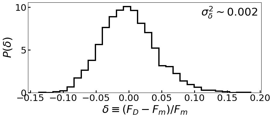
In Figure 2, we show an example of the observed and residual counts for one of our patches. In addition, we show a histogram of the relative fluctuation of the residual counts map for the same patch. The rms of the fluctuation being is . Note that we confirm that our patches do not contain new point sources with test statistics (TS) larger than 25.
Once reconstructed the UGRB, we estimate the putative flux of each LSBG. According to the prescription described in the 2FGL catalog, the Bayesian method [59] should be applied for the likelihood analysis of very faint sources [60]. We introduce free parameters representing the -th point-source flux-amplitude in -th energy bin. Here we define TS as and is given by;
| (7) |
where and are the LAT data and the nuisance parameters of all the -ray sources other than our target LSBGs. The best fit parameters are obtained when is maximized. In the above equation means no target source. We checked that the TS values of all our LSBGs are less than 1 for most energy bins, which justifies our choice of using the Bayesian method introduced in [7].

IV Result
IV.1 Composite analysis
As described in Section III.3.2, because of the very low -ray signal of our LSBGs, we compute the 95% C.L. upper limits on the DM annihilation cross-section parameter using the same approach as in [36]. Since all likelihood values obtained at each object are assumed to be independent of each other, the composite likelihood for the full sample of targets can be expressed as follows;
| (8) |
where is the -factor of the -th target and the index runs over all energy bins. is the log-likelihood value for the -th LSBG, which is obtained by the difference of the log-likelihood value from the one in the case of no source.
Now we calculate the J-factor for each object to evaluate the model flux described in Section II.1. For the simplicity of Equation 2, we need to consider the relationship between the PSF of the LAT instrument and the angular size of objects. The PSF (68% containment angles) decreases from to as -ray energy increases from 500 MeV to 500 GeV. The angular size of LSBG is smaller than a few 10 arcsecs, hence smaller than the PSF in all energy bands. Therefore, we can consider them as point-like sources in the likelihood computation. Then, the integration of over the target volume in Equation 2 is reduced to;
| (9) |
where is the angular diameter distance to the object, which is given by assignment of distance randomly drawn followed the measured distribution. Then, Equation 9 is straightforwardly calculated;
| (10) | ||||
where is the spherical overdensity set to be 200 and is the critical density at the redshift. Since our targets are regarded as point sources, our assumption is correct if the angular separations between objects are larger than the LAT PSF over all considered energy ranges; otherwise, it is incorrect because their mean surface number density is about 4 per . We will further discuss the parameter correlation between neighboring objects in Section V.1. In our procedure, we assume that the LSBG flux is positive definite, which implies that the data are well-described by a distribution rather than . As such, the 95% C.L. upper limits on the cross section are given when the .
IV.2 measurement
Following the methodology described in Subsection II.2, we estimate the distribution of the HSC-LSBG sample. For this, we divide the reference redshift sample into five equally-separated bins from to . Then, we compute the cross correlation between the sample in each bin and the entire LSBG sample. The angular cross correlation is computed in the angular bin , which is further divided in smaller logarithmic-scaled bins. We use the estimator [61],
| (11) |
where or represent the normalized number of pairs separated within the th angular bin between data and data or data and random, respectively (in our case, “data” and “random” represent the spec-z or LSBG samples in our datasets and the corresponding random samples, respectively). Subscripts , and represent the photometric sample, and reference sample in the th redshift bin, respectively.
The rest of the subsection is devoted to describing the covariance of the estimation, which will be used to draw the galaxy redshift randomly from the distribution. We estimate the covariance of using the Jackknife method [62] as
| (12) |
where is the angular correlation function for the th Jackknife sub-sample in the -th angular and -th redshift bins. is the number of the Jackknife sub-samples, and we take which divides the entire region into deg2 patches. is the averaged correlation function over all jackknife sub-samples,
| (13) |
Now the at the -th redshift bin can be obtained by integrating along the angular scale, and its amplitude can be considered as a parameter . Therefore, the distribution can be stochastically determined with the likelihood function of , which is assumed to be Gaussian, possibly with a physically reasonable prior or otherwise. The variance of the Gaussian likelihood function can be derived as
| (14) |
where can be computed using Equation 5. Figure 3 represents the distribution measurement. The errors are measured using the Jackknife resampling. For the clustering analysis described in this section, we use a publicly available code, treecorr [63].

IV.3 Evaluation of statistical uncertainty
The upper limit on the cross section in the composite analysis can be affected by the measurement error and the halo property estimation, which is specified by the halo mass and concentration parameter as described in Section IV.1. We evaluate the coverage of the upper limits by using 500 Monte Carlo simulations. First, for the halo mass, we evaluate its uncertainty as at 1- Gaussian error by computing the scatter of stellar-to-halo-mass conversion. In addition, we adopt a concentration parameter error of of at 1- Gaussian error [64]. Accordingly, the total uncertainty for halo properties results in -factor uncertainties of 0.9 dex at 1- error. Moreover, we randomly assign the distance to galaxies according to this distribution; therefore, the negative values of the amplitude are physically unreasonable. Therefore, as described in the previous section, we obtain the posterior function of as . We finally apply linear interpolation between each center of redshift bin to the posterior distribution. We take a conservative limit of the minimum redshift of the sample corresponding to 25 Mpc, which is the minimum distance among the HSC-LSBG samples with precisely measured distance.
In Figure 4, we show the total J-factor values as a function of the number of stacked objects, . In the order of square, cross and circle symbols, the error-bars plot the total values including measurement uncertainty, halo property and both, respectively. For comparison with other studies, we display at the 95% C.L. for a DM mass of 1 TeV in the right axis, and their corresponding J-factor value on the left axis. Note that when converting the J-factor to , we apply a mean flux of our UGRB sky. The upper limit is affected by both the fluctuation and target’s -factor value, however we find that, even in the lower energy regime, the scatter by the fluctuation is smaller (0.4 dex at 2- level) than the total halo property and measurement uncertainty.

V Discussion
V.1 Correlation between neighbors
We performed the composite analysis in Section IV.1 assuming that the likelihood functions of individual objects are independent of each other. Such correlations are expected when the number density of the sample is high because the PSF of Fermi-LAT is . In this subsection, we demonstrate that the correlation between data at different points can be negligible.
In the HSC-Fermi sky coverage, we select 10 independent patches with the size of deg2. From each patch, we randomly select 60 pairs of points with separations of 0.5∘ to 3∘. To evaluate the correlation between the putative flux amplitudes of the paired objects, we perform the joint likelihood analysis for the pairs, which simultaneously optimizes the fluxes of the paired objects. The putative flux of an object is defined by,
| (15) |
We fit the amplitude parameters to the UGRB flux and measure the covariance matrix using the fit and sed methods in fermipy. Figure 5 shows the absolute value of the correlation between two amplitude parameters in the overall energy ranges, as the function of the separation. The error-bars are computed from the 60 independent pairs that reflects the fluctuations of the residual gamma-ray flux. The cross-covariance is normalized by the diagonal terms, i.e., . Although we expect a strong correlation on scales smaller than 1 deg, the correlation at the smallest separation, which corresponds to the HSC-LSBG mean separation, is less than 0.1 deg at 1- level. We note that all the cross correlation values are negative at all scales, which is the consequence of the conservation of the total flux. For further validation, we perform a composite likelihood analysis in which we obtain the likelihood profiles for the putative fluxes of all samples within a single LAT data patch simultaneously. Figure 6 compares the constraints with this simultaneous approach (‘simultaneous’ case) with the one obtained based on the assumption that all objects are independent of each other (‘independent’ case). We emphasize that the ‘independent’ case gives a weaker constraint on than the ‘simultaneous’ case. This is because the total flux conservation is imposed, which results in a larger putative flux amplitude for the ‘independent’ case. Note that in this calculation, we set all objects’ J-factor to , and choose a specific . This explains why the amplitudes of in Figure 6 do not correspond to the ones in Figure 4.
We conclude that the correlation between neighboring points is less than , on scales of order 0.5 deg. Even if we ignore this correlation, which is computationally much less expensive, we would obtain conservative constraints on the .


V.2 The power of stacking
In this subsection, we discuss a scaling relation of the statistical power on as a function of the number of objects included in the stacking procedure. We first analytically show that is proportional to the inverse of in the limit of zero observed photon counts. We then also demonstrate that this scaling relation converges to independent of the DM mass if the is sufficiently large by using HSC-LSBG catalog and Fermi observations.
Let us first revisit the Poisson likelihood for a single LSBG in the UGRB. The likelihood function for the model parameters is given by the Poisson distribution,
| (16) |
where the index runs over all energy bins and pixels and is the observed photon counts; is expected photon counts for model fluxes, which is decomposed into the Galactic foreground, isotropic background and resolved point-source model fluxes as well as the flux by the DM annihilation for the single LSBG. A UGRB sky is derived from the modeling of all the -ray sources except for the LSBG flux as described in Section III.3.2. Therefore, if we fix the model parameters of the background sky, then depends only on the parameter . We denote , where is the total model flux of all sources without LSBG and is the model flux of LSBG. For simplicity, we consider that all LSBGs have the same J-factor, which means that their model fluxes are equal. In addition, we consider the fact that, in energy regimes higher than 30 GeV, the LAT hardly detects photons. Given that there is no photon count () in such energy regimes and in all pixels, we expect and then . Consequently, we obtain the composite likelihood with objects using Equation 8,
| (17) |
where is the number of objects in the composite analysis. Thus, in our approach the upper limit is proportional to since .
Further, we explore the scaling relation using the HSC-LSBG catalog and Fermi data. We calculate the constraint on from randomly drawn objects from the HSC-LSBG sample. Because here we aim to isolate the effect of number of stacking from the individual halo properties, we assume the selected sample has a same factor, but using the actual background -ray fluxes at that position. We repeat this calculation 500 times for each sampling. In Figure 7, we show the median value of the ratio of with objects to the one with a single object for DM mass of 10 GeV, 100 GeV and 1 TeV. With larger than 30, the upper limits scale with the inverse of for all mass ranges. We have discussed this relation in our previous paper [36], which predicted the relation based only on 8 HSC LSBGs . In this paper, we confirm that prediction of scaling with , but furthermore we find, thanks to the large number of LSBG sample, that the relation is independent of DM mass. This is because most of the constraints are dominated by the objects having significantly low background fluxes. Such objects can be found with a certain probability, say of the entire sample. Therefore, when the number of stacking objects is small, e.g. , the probability of having strongly constrained objects is less than , and the constraining power does not scale with . However, the probability of having such objects may increase and converge to . as we increase the number of stacking. Therefore, the statistical power of stacking, dominated by the objects with almost zero-background fluxes scales with . For DM mass of 100 GeV and 1 TeV, this scaling relation is seen, even in smaller . This behavior is reasonable, considering the photon-count statistics in a high energy regime. The annihilation process with more massive DM particles can produce higher energy photons, thus probing the DM annihilation for more massive DM is affected by photon-count statistics in high energy regimes.

VI Conclusions
In this study, we proposed a new method to constrain the DM annihilation cross-section with potential -ray sources with unknown redshifts and the observed -ray background. The crucial point is that we do not need to know the individual distance to the -ray sources. The overall redshift distribution is sufficient to constrain the DM annihilation cross section. By applying the redshift clustering method, we obtained a redshift distribution of the whole population, instead of the redshifts of individual objects. We then randomly assigned the distance to each LSBG according to this distribution. To validate the proposed method, we measured of full samples of the HSC-LSBG catalog including 800 objects and constrained the DM annihilation cross-section via a composite likelihood analysis using all LSBGs given distances and using the eight years of Fermi-LAT observations.
In the measurement for the LSBG samples, we employed the NSA catalog as spec-z samples in overlapped regions with the HSC region. The uncertainty in the was evaluated with Monte Carlo simulations. We found that in the composite analysis with 1000 objects, uncertainties of the halo property estimation and measurement are quite small and not significantly affected to the upper limit on the cross section. Therefore, using distribution of overall target samples instead of the individual sample’s redshifts is a valid and robust approach for the DM signal search.
To reduce the computational cost, we assumed that all the spectral parameters of the different LSBGs are independent of each other. The number density of the LSBGs () was comparable to the LAT PSF scale, which may lead to a correlation between spectral parameters for neighboring LSBGs, and thus may break the assumption. We validated this conjecture in two ways. First, we computed the covariance matrix between the two normalizations for each paired neighbor and checked that off-diagonals terms of the correlation matrix is smaller than 0.1 at the separation angle . Second, fixing the J-factor and distance of each object, we performed a composite likelihood analysis in which we obtained the likelihood profiles for putative fluxes of all samples in each LAT patch simultaneously. By comparing , we found that the constraints differ at most by a factor of 2. Moreover, if we assume that the data is independent, then the constraints become more conservative due to the relaxation of the total flux conservation condition.
Finally, we found the scaling relation of with the number of objects in the composite likelihood analysis. First, under an assumption of zero observed photon, we discussed the relation analytically and found that is proportional to .Furthermore, using the real HSC-LSBG catalog and the LAT data, we computed the scaling for DM mass of 10 GeV, 100 GeV and 1 TeV and showed that for all DM masses the upper limit scales with using . This is a significant effect which is the consequence of the Poisson statistics due to rare photons detected by the LAT and is different from the Gaussian statistics in which the scaling obeys .
In future imaging surveys with next-generation telescopes such as the LSST, a large number of LSBGs will be detected because of wider sky coverage and better sensitivity. For example, LSST has a sky coverage of 20,000 deg2 and reaches the depth of 27.5 in band and consequently has the potential to discover objects. Although, for the reference samples we need spec-z or high-precision photo-z samples located in the local universe, it is expected that these will decrease the uncertainties in the estimate of due to the measurement and the halo properties. Moreover, by increasing the statistics, we can perform a more detailed measurement, particularly in a redshift range corresponding to a distance of less than 25 Mpc, which is the minimum distance adopted here for a conservative J-factor estimate in our likelihood procedure. We expect that in the future, this will give a more stringent constraint on the DM cross-section.
Acknowledgements.
This work was supported in part by World Premier International Research Center Initiative, MEXT, Japan, and JSPS KAKENHI Grant No. 19H00677, 20H05850, 20H05855, 20J11682 and 21H05454.References
- [1] G. Jungman, M. Kamionkowski, and K. Griest. Supersymmetric dark matter. Physics Report, 267:195–373, Mar 1996.
- [2] Gianfranco Bertone, Dan Hooper, and Joseph Silk. Particle dark matter: evidence, candidates and constraints. Physics Report, 405(5-6):279–390, Jan 2005.
- [3] Giorgio Arcadi, Maíra Dutra, Pradipta Ghosh, Manfred Lindner, Yann Mambrini, Mathias Pierre, Stefano Profumo, and Farinaldo S. Queiroz. The waning of the WIMP? A review of models, searches, and constraints. European Physical Journal C, 78(3):203, March 2018.
- [4] Leszek Roszkowski, Enrico Maria Sessolo, and Sebastian Trojanowski. WIMP dark matter candidates and searches—current status and future prospects. Reports on Progress in Physics, 81(6):066201, Jun 2018.
- [5] Tongyan Lin. TASI lectures on dark matter models and direct detection. arXiv e-prints, page arXiv:1904.07915, Apr 2019.
- [6] Gary Steigman, Basudeb Dasgupta, and John F. Beacom. Precise relic wimp abundance and its impact on searches for dark matter annihilation. Phys. Rev. D, 86:023506, Jul 2012.
- [7] The Fermi-LAT collaboration. Fermi Large Area Telescope Fourth Source Catalog. arXiv e-prints, page arXiv:1902.10045, Feb 2019.
- [8] C. Gordon and O. Macías. Dark matter and pulsar model constraints from Galactic Center Fermi-LAT gamma-ray observations. Phys. Rev. D, 88(8):083521, October 2013.
- [9] K. N. Abazajian, N. Canac, S. Horiuchi, and M. Kaplinghat. Astrophysical and dark matter interpretations of extended gamma-ray emission from the Galactic Center. Phys. Rev. D, 90(2):023526, July 2014.
- [10] F. Calore, I. Cholis, and C. Weniger. Background model systematics for the Fermi GeV excess. JCAP, 3:038, March 2015.
- [11] T. Daylan, D. P. Finkbeiner, D. Hooper, T. Linden, S. K. N. Portillo, N. L. Rodd, and T. R. Slatyer. The characterization of the gamma-ray signal from the central Milky Way: A case for annihilating dark matter. Physics of the Dark Universe, 12:1–23, June 2016.
- [12] Ackermann, M. et al. The Fermi Galactic Center GeV Excess and Implications for Dark Matter. Astrophys. J. , 840(1):43, May 2017.
- [13] Ackermann, M. et al. Searching for Dark Matter Annihilation from Milky Way Dwarf Spheroidal Galaxies with Six Years of Fermi Large Area Telescope Data. Phys. Rev. Lett. , 115(23):231301, Dec 2015.
- [14] Albert, A. et al. Searching for Dark Matter Annihilation in Recently Discovered Milky Way Satellites with Fermi-Lat. Astrophys. J. , 834(2):110, Jan 2017.
- [15] V. Gammaldi, E. Karukes, and P. Salucci. Theoretical predictions for dark matter detection in dwarf irregular galaxies with gamma rays. Phys. Rev. D, 98(8):083008, Oct 2018.
- [16] S. Hoof, A. Geringer-Sameth, and R. Trotta. A Global Analysis of Dark Matter Signals from 27 Dwarf Spheroidal Galaxies using Ten Years of Fermi-LAT Observations. arXiv e-prints, December 2018.
- [17] Kimberly K. Boddy, Jason Kumar, Danny Marfatia, and Pearl Sand ick. Model-independent constraints on dark matter annihilation in dwarf spheroidal galaxies. Phys. Rev. D, 97(9):095031, May 2018.
- [18] Sebastian Hoof, Alex Geringer-Sameth, and Roberto Trotta. A global analysis of dark matter signals from 27 dwarf spheroidal galaxies using 11 years of Fermi-LAT observations. JCAP, 2020(2):012, February 2020.
- [19] K. Belotsky, A. Kirillov, and M. Khlopov. Gamma-ray evidence for dark matter clumps. Gravitation and Cosmology, 20(1):47–54, Jan 2014.
- [20] S. Ando and E. Komatsu. Constraints on the annihilation cross section of dark matter particles from anisotropies in the diffuse gamma-ray background measured with Fermi-LAT. Phys. Rev. D, 87(12):123539, June 2013.
- [21] Mattia Fornasa and Miguel A. Sánchez-Conde. The nature of the Diffuse Gamma-Ray Background. Physics Report, 598:1–58, October 2015.
- [22] Shin’ichiro Ando, Aurélien Benoit-Lévy, and Eiichiro Komatsu. Mapping dark matter in the gamma-ray sky with galaxy catalogs. Phys. Rev. D, 90(2):023514, Jul 2014.
- [23] Ackermann, M. et al. The Spectrum of Isotropic Diffuse Gamma-Ray Emission between 100 MeV and 820 GeV. Astrophys. J. , 799:86, January 2015.
- [24] Ajello, M. et al. The Origin of the Extragalactic Gamma-Ray Background and Implications for Dark Matter Annihilation. Astrophys. J. , 800(2):L27, Feb 2015.
- [25] J. Kataoka, M. Tahara, T. Totani, Y. Sofue, Y. Inoue, S. Nakashima, and C. C. Cheung. Global Structure of Isothermal Diffuse X-Ray Emission along the Fermi Bubbles. Astrophys. J. , 807(1):77, Jul 2015.
- [26] Alessandro Cuoco, Jun-Qing Xia, Marco Regis, Enzo Branchini, Nicolao Fornengo, and Matteo Viel. Dark Matter Searches in the Gamma-ray Extragalactic Background via Cross-correlations with Galaxy Catalogs. ApJS, 221(2):29, December 2015.
- [27] Marco Regis, Jun-Qing Xia, Alessandro Cuoco, Enzo Branchini, Nicolao Fornengo, and Matteo Viel. Particle Dark Matter Searches Outside the Local Group. Phys. Rev. Lett. , 114(24):241301, June 2015.
- [28] Masato Shirasaki, Oscar Macias, Shunsaku Horiuchi, Satoshi Shirai, and Naoki Yoshida. Cosmological constraints on dark matter annihilation and decay: Cross-correlation analysis of the extragalactic -ray background and cosmic shear. Phys. Rev. D, 94(6):063522, September 2016.
- [29] Tilman Tröster, Stefano Camera, Mattia Fornasa, Marco Regis, Ludovic van Waerbeke, Joachim Harnois-Déraps, Shin’ichiro Ando, Maciej Bilicki, Thomas Erben, Nicolao Fornengo, Catherine Heymans, Hendrik Hildebrandt, Henk Hoekstra, Konrad Kuijken, and Massimo Viola. Cross-correlation of weak lensing and gamma rays: implications for the nature of dark matter. MNRAS, 467(3):2706–2722, May 2017.
- [30] Mariangela Lisanti, Siddharth Mishra-Sharma, Nicholas L. Rodd, and Benjamin R. Safdi. Search for Dark Matter Annihilation in Galaxy Groups. Phys. Rev. Lett. , 120(10):101101, March 2018.
- [31] Mariangela Lisanti, Siddharth Mishra-Sharma, Nicholas L. Rodd, Benjamin R. Safdi, and Risa H. Wechsler. Mapping extragalactic dark matter annihilation with galaxy surveys: A systematic study of stacked group searches. Phys. Rev. D, 97(6):063005, March 2018.
- [32] Ackermann, M. et al. Unresolved Gamma-Ray Sky through its Angular Power Spectrum. Phys. Rev. Lett. , 121(24):241101, Dec 2018.
- [33] Daiki Hashimoto, Atsushi J. Nishizawa, Masato Shirasaki, Oscar Macias, Shunsaku Horiuchi, Hiroyuki Tashiro, and Masamune Oguri. Measurement of redshift-dependent cross-correlation of HSC clusters and Fermi -rays. MNRAS, 484(4):5256–5266, Apr 2019.
- [34] Pooja Bhattacharjee, Pratik Majumdar, Mousumi Das, Subinoy Das, Partha S. Joarder, and Sayan Biswas. Multiwavelength analysis of low surface brightness galaxies to study possible dark matter signature. MNRAS, 501(3):4238–4254, March 2021.
- [35] Charles Thorpe-Morgan, Denys Malyshev, Christoph-Alexander Stegen, Andrea Santangelo, and Josef Jochum. Annihilating dark matter search with 12 yr of Fermi LAT data in nearby galaxy clusters. MNRAS, 502(3):4039–4047, April 2021.
- [36] Daiki Hashimoto, Oscar Macias, Atsushi J. Nishizawa, Kohei Hayashi, Masahiro Takada, Masato Shirasaki, and Shin’ichiro Ando. Constraining dark matter annihilation with HSC low surface brightness galaxies. JCAP, 2020(1):059, January 2020.
- [37] Carolin Wittmann, Thorsten Lisker, Liyualem Ambachew Tilahun, Eva K. Grebel, Christopher J. Conselice, Samantha Penny, Joachim Janz, John S. Gallagher, Ralf Kotulla, and James McCormac. A population of faint low surface brightness galaxies in the Perseus cluster core. MNRAS, 470(2):1512–1525, Sep 2017.
- [38] Wei Du, Cheng Cheng, Hong Wu, Ming Zhu, and Yougang Wang. Low Surface Brightness Galaxy catalogue selected from the .40-SDSS DR7 Survey and Tully-Fisher relation. MNRAS, 483(2):1754–1795, February 2019.
- [39] D. J. Prole, M. Hilker, R. F. J. van der Burg, M. Cantiello, A. Venhola, E. Iodice, G. van de Ven, C. Wittmann, R. F. Peletier, S. Mieske, M. Capaccioli, N. R. Napolitano, M. Paolillo, M. Spavone, and E. Valentijn. Halo mass estimates from the globular cluster populations of 175 low surface brightness galaxies in the Fornax cluster. MNRAS, 484(4):4865–4880, Apr 2019.
- [40] J. P. Greco, J. E. Greene, M. A. Strauss, L. A. Macarthur, X. Flowers, A. D. Goulding, S. Huang, J. H. Kim, Y. Komiyama, A. Leauthaud, L. Leisman, R. H. Lupton, C. Sifón, and S.-Y. Wang. Illuminating Low Surface Brightness Galaxies with the Hyper Suprime-Cam Survey. Astrophys. J. , 857:104, April 2018.
- [41] Tesla E. Jeltema and Stefano Profumo. Fitting the Gamma-Ray Spectrum from Dark Matter with DMFIT: GLAST and the Galactic Center Region. JCAP, 0811:003, 2008.
- [42] N. Hiroshima, S. Ando, and T. Ishiyama. Modeling evolution of dark matter substructure and annihilation boost. Phys. Rev. D, 97(12):123002, June 2018.
- [43] J. F. Navarro, C. S. Frenk, and S. D. M. White. The Structure of Cold Dark Matter Halos. Astrophys. J. , 462:563, May 1996.
- [44] Benedikt Diemer and Michael Joyce. An Accurate Physical Model for Halo Concentrations. Astrophys. J. , 871(2):168, February 2019.
- [45] Benedikt Diemer. COLOSSUS: A Python Toolkit for Cosmology, Large-scale Structure, and Dark Matter Halos. ApJS, 239(2):35, December 2018.
- [46] Jester, S. et al. The Sloan Digital Sky Survey View of the Palomar-Green Bright Quasar Survey. AJ, 130:873–895, September 2005.
- [47] J. Woo, S. Courteau, and A. Dekel. Scaling relations and the fundamental line of the local group dwarf galaxies. MNRAS, 390:1453–1469, November 2008.
- [48] B. P. Moster, T. Naab, and S. D. M. White. Galactic star formation and accretion histories from matching galaxies to dark matter haloes. MNRAS, 428:3121–3138, February 2013.
- [49] Jeffrey A. Newman. Calibrating Redshift Distributions beyond Spectroscopic Limits with Cross-Correlations. Astrophys. J. , 684(1):88–101, September 2008.
- [50] Brice Ménard, Ryan Scranton, Samuel Schmidt, Chris Morrison, Donghui Jeong, Tamas Budavari, and Mubdi Rahman. Clustering-based redshift estimation: method and application to data. arXiv e-prints, page arXiv:1303.4722, March 2013.
- [51] Michael R. Blanton, Eyal Kazin, Demitri Muna, Benjamin A. Weaver, and Adrian Price-Whelan. Improved Background Subtraction for the Sloan Digital Sky Survey Images. AJ, 142(1):31, July 2011.
- [52] Miyazaki, S. et al. Hyper Suprime-Cam: System design and verification of image quality. PASJ, 70:S1, January 2018.
- [53] Komiyama, Y. et al. Hyper Suprime-Cam: Camera dewar design. PASJ, 70:S2, January 2018.
- [54] Aihara, Hiroaki et al. Second data release of the Hyper Suprime-Cam Subaru Strategic Program. PASJ, 71(6):114, December 2019.
- [55] Feng-Jie Lei, Hong Wu, Yi-Nan Zhu, Wei Du, Min He, Jun-Jie Jin, Pin-Song Zhao, and Bing-Qing Zhang. An H Imaging Survey of the Low Surface Brightness Galaxies Selected from the Spring Sky Region of the 40% ALFALFA H I Survey. ApJS, 242(1):11, May 2019.
- [56] Atwood, W. et al. Pass 8: Toward the Full Realization of the Fermi-LAT Scientific Potential. arXiv e-prints, page arXiv:1303.3514, March 2013.
- [57] Ackermann, M. et al. The Fermi Large Area Telescope on Orbit: Event Classification, Instrument Response Functions, and Calibration. ApJS, 203:4, November 2012.
- [58] M. Wood, R. Caputo, E. Charles, M. Di Mauro, J. Magill, J. S. Perkins, and Fermi-LAT Collaboration. Fermipy: An open-source Python package for analysis of Fermi-LAT Data. International Cosmic Ray Conference, 301:824, Jan 2017.
- [59] O. Helene. Upper limit of peak area. Nuclear Instruments and Methods in Physics Research, 212(1-3):319–322, Jul 1983.
- [60] Nolan, P. L. et al. Fermi Large Area Telescope Second Source Catalog. ApJS, 199(2):31, Apr 2012.
- [61] S. D. Landy and A. S. Szalay. Bias and variance of angular correlation functions. Astrophys. J. , 412:64–71, July 1993.
- [62] Scranton, R. et al. Analysis of Systematic Effects and Statistical Uncertainties in Angular Clustering of Galaxies from Early Sloan Digital Sky Survey Data. Astrophys. J. , 579:48–75, November 2002.
- [63] Mike Jarvis. TreeCorr: Two-point correlation functions, August 2015.
- [64] A. A. Dutton and A. V. Macciò. Cold dark matter haloes in the Planck era: evolution of structural parameters for Einasto and NFW profiles. MNRAS, 441:3359–3374, July 2014.