D2S: Representing sparse descriptors and 3D coordinates for camera relocalization
Abstract
State-of-the-art visual localization methods mostly rely on complex procedures to match local descriptors and 3D point clouds. However, these procedures can incur significant costs in terms of inference, storage, and updates over time. In this study, we propose a direct learning-based approach that utilizes a simple network named D2S to represent complex local descriptors and their scene coordinates. Our method is characterized by its simplicity and cost-effectiveness. It solely leverages a single RGB image for localization during the testing phase and only requires a lightweight model to encode a complex sparse scene. The proposed D2S employs a combination of a simple loss function and graph attention to selectively focus on robust descriptors while disregarding areas such as clouds, trees, and several dynamic objects. This selective attention enables D2S to effectively perform a binary-semantic classification for sparse descriptors. Additionally, we propose a simple outdoor dataset to evaluate the capabilities of visual localization methods in scene-specific generalization and self-updating from unlabeled observations. Our approach outperforms the previous regression-based methods in both indoor and outdoor environments. It demonstrates the ability to generalize beyond training data, including scenarios involving transitions from day to night and adapting to domain shifts.
I Introduction
Visual re-localization plays a crucial role in numerous applications including robotics and computer vision. The majority of methods rely on sparse reconstruction models, and local feature matching [1, 2]. The 3D reconstructed model, commonly built using Structure from Motion (SfM), stores 3D points cloud map along with local and global visual descriptors [1, 3, 4, 2]. While showing superior performance in handling appearance changes introduced by different devices and viewpoints, these methods suffer from several drawbacks. First, point clouds and visual descriptors need to be stored explicitly, which hinders their practicality to large-scale scenes due to storage requirements. Second, the involvement of multiple components such as feature extraction and feature matching make these approaches computation-extensive which is not suitable for execution on consumer or edge devices.
Conversely, end-to-end learning of the implied 2D–3D correspondences offers a better trade-off between accuracy and computational efficiency [5, 6, 7]. These approaches, commonly referred to as scene coordinate regression (SCR), directly regressing scene coordinates from corresponding 2D pixels of the input image. Thus, SCRs naturally establish the 2D–3D matches without the need for the 3D models but it is worth mentioning that they are prone to overfitting if the training data does not adequately represent the environment [8]. Although previous SCR-based approaches have demonstrated high accuracy for re-localization in small-scale and stationary environments [5, 9, 7], their performance are not on par with feature matching (FM)-based methods in environments that contain variations over a long span of time [10] and high domain shift scenarios.

In this study, we introduce a new visual localization approach named D2S that leverages keypoint descriptors to address the aforementioned issues of previous SCR methods. Instead of learning directly from RGB images, we initiate the regression network from sparse salient descriptors. This allows the network to learn the mapping between keypoint descriptors and their corresponding scene coordinates. By exploiting the self-attention mechanism, we also enable D2S to learn the global context by communicating between features. As a result, D2S inherits the robustness of salient features, making it resilient against drastic changes in the environment. In addition, we explore an aspect that previous SCR research [7, 11] lacks, which is the ability of the model to utilize new, unlabeled data from various devices. We propose a simple yet efficient self-supervised technique for updating the re-localizer with unlabeled observations, which further enhances D2S’s ability to accommodate dynamic environments. In Fig. 1, we present a summary of the proposed pipeline. Our contributions can be listed as follows:
-
•
We introduce D2S (Descriptors to Scenes), a novel lightweight network for representing sparse descriptors and 3D coordinates, enabling real-time, high-precision re-localization.
-
•
The proposed D2S combines graph attention with a simple loss function to identify reliable descriptors, enabling a strong focus on robust descriptors and improving re-localization performance.
-
•
We show that D2S can seamlessly self-update with new observations without requiring camera poses, parameters, or ground truth scene coordinates. To this end, we introduce a small challenge dataset to evaluate the method in scenarios of high domain shift, sparse training data, and self-updating with unlabeled data.
-
•
We present a comprehensive evaluation of the proposed D2S across three indoor and outdoor datasets, demonstrating that our method outperforms the state of the art.
II Related Work
II-A Image Retrieval and Absolute Pose Regression
Image-based visual re-localization methods[12] were arguably the simplest solution, which constructing maps just by storing a set of images and their camera pose in a database. Given a query image, we seek for the most similar images in the database by comparing their global descriptor [4, 13]. With the matched images representing a location in a scene that is close to the query image [13, 4], the pose of the query image can be derived from the top retrieved images pose. Despite demonstrating scalability in large environments, these approaches have limited accuracy in determining camera poses. Thus they are often used as initialization for later pose refinements.
6DoF absolute camera pose regression approaches (APR) have been studied extensively to overcome the drawbacks of image retrieval. Notably, PoseNet[14] was first proposed, along with subsequent developments [14, 15, 16]. APR learns to directly encode the 6DoF camera pose from the image, resulting in a lightweight system where memory demand and estimation time are independent of the reference data size. However, theoretical conclusions [17] suggest that APR behaviors are more closely related to image retrieval than methods that estimate poses by 3D geometry. Thus APR could hardly outperform a handcraft retrieval baseline.
II-B Sparse Feature Matching
Features matching-based (FM) re-localizers compute the camera pose from 2D-3D correspondences between 2D pixels and 3D scene maps, constructed using Structure-from-Motion (SfM) [18, 2]. Early FM-based solutions match local descriptors in 2D images to 3D points in the SfM model [19, 20, 21, 22]. Despite achieving accurate pose estimations, exhaustive matching creates a substantial computational bottleneck. Additionally, as SfM models grow in size, direct matching becomes ambiguous and difficult to establish under significant appearance changes. Leveraging the robustness of image retrieval in scalability and handling appearance changes, [2, 23] proposed a hierarchical re-localization approach that uses image retrieval as an initialization step before performing 2D-3D direct matching. Instead of performing complex 2D-3D matching, [24] proposed deep feature alignment, reducing system complexity while preserving accurate estimation.
II-C Scene Coordinate Regression
Compared to the FM-based pipeline, scene coordinate regression (SCR) approaches are more straightforward. By employing a single regression network, 3D coordinates can be directly extracted from 2D pixels [5, 9, 6, 7, 11]. These correspondences then serve as the input for RANSAC-based pose optimization. SCR methods have demonstrated superior accuracy in camera pose estimation in small-scale and stationary environments. However, scaling these methods to larger, dynamic environments remains challenging. They struggle with adapting to novel viewpoints and handling the increased complexity that comes with larger-scale environments [10]. Our proposed model, adopting similar idea to SCR but aim to address the aforementioned problem. By utilizing the robustness of local keypoint descriptors, our model seeks to enhance performance in high viewpoint changes and dynamic scenarios.
II-D Self-Supervised Updating with Unlabeled Data
Visual SLAM systems [25] allow continuous map updates, but most visual re-localization techniques, including FM [2, 26] and SCR-based methods [9, 6, 7, 11], lack such adaptability, requiring reconstruction and labeling for updates. APR-based approaches have pioneered self-supervised updates with unlabeled data, utilizing sequential frames [27] or feature matching [16]. ACE0 [28] represents the first SCR-based method to introduce this capability but remains limited under highly dynamic conditions [10]. In this study, we demonstrate that the proposed sparse regression-based D2S adapts naturally to such conditions through self-supervision without needing reconstruction or labeling.
III Proposed Approach
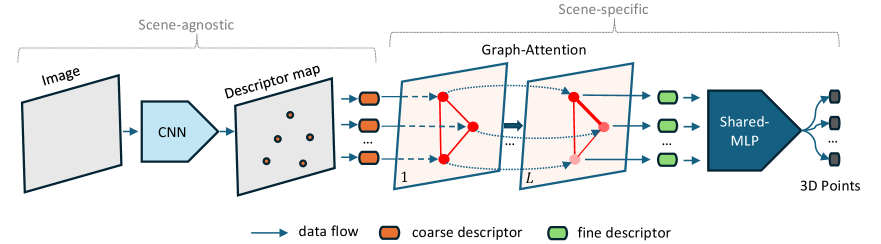
Given a set of reference images and its reconstructed SfM model , we aim to develop a sparse regression module, which can encode the entire environment using a compact function , where is a deep neural network. The proposed function inputs a set of local descriptors extracted from and outputs its corresponding 3D global cloud coordinates . The ultimate goal of the proposed module is to perform visual localization, a task of estimating camera pose of the query image . We illustrate the proposed architecture in Fig. 2.
III-A Representing Sparse Descriptors and 3D Coordinates
Inspired by the universal continuous set function approximator [29], we first propose a simple element set learning function . It receives a set of descriptors as input and outputs corresponding scene coordinates . Overall, the proposed function can be described as follows:
| (1) | ||||
where and . is the number of descriptors, and is descriptor dimension. The function is a shared nonlinear function. It receives a descriptor vector and outputs a scene coordinate vector . We introduce an additional dimension for the scene coordinate, which represents the reliability probability for localization of the input descriptor . To ensure that the range of the reliability probability output lies within while enabling function to produce , we compute the final reliability prediction using the following equation:
| (2) |
where is a scale factor chosen to make the expected value of reliability prediction easy to reach a small value when the input descriptors belong to high uncertainty regions.
The proposed module is theoretically simple. As illustrated in Eq. 1, it requires only a non-linear function to compute the scene coordinates of given descriptors. In practice, we approximate using a multi-layer perceptron (MLP) network, which is similar to [11].

III-B Optimizing with Graph Attention
Solely relying on independent descriptors to regress scene coordinates may lead to an insufficient understanding of the global context and the distinctiveness of feature clusters. To address this issue, we draw inspiration from recent works on feature matching [23], which leverage attention aggregation [30] to learn both local and global attributes of sparse features. We employ a simplified version for the scenes regression task, which can be described as follows:
| (3) | ||||
where , and represents a nested residual attention update for each descriptor across graph layers. Given a coarse local descriptor , is used to compute its fine regression descriptor by letting it communicate with each other across attention layers. This implicitly incorporates visual relationships and contextual cues with other descriptors in the same image, enabling it to extract robust features automatically through an end-to-end learning pipeline from scene coordinates. In addition, the proposed reliability-aware detection, as described in Eq. 2, can also encourage our attention module to favor features from reliable areas (e.g. buildings, stable objects) and suppress those from unreliable regions (e.g. trees, sky, human).
As is the representation for the output regression descriptor of element at layer , Eq. 3 can be simplified as follows:
| (4) |
which now has a similar form to the original Eq. 1, where the final regression layer is simply a shared MLP.
Similar to a previous study [23], we also consider the attentional module as a multi-layer graph neural network. However, we only leverage the self-edge, which is based on self-attention [30], to connect the descriptor to all others in the same image. The message passing formulation for element at the layer is described as
| (5) |
where denotes the aggregated message result from all descriptors , with indicating the set of descriptor indices, and denoting concatenation. This module consists of chained layers with different parameters. Therefore, the message is different in each layer.
The self-attention mechanism performs an interaction to map the query vector against a set of key vectors , associated with candidate descriptors, to compute the attention score Softmax. It then presents the best-matched descriptors with their value vectors represented by a scored average of values, which in practice is the computation of message :
| (6) |
The query, key, and value are derived from linear projections between the descriptor with three different weight matrices , , and . This linear projection for all descriptors is expressed as
| (7) |
III-C Updating D2S with Unlabeled Observations
-
-
training images,
-
-
training descriptors,
-
-
training scene coordinates,
-
-
unlabeled images,
-
-
unlabeled descriptors,
-
-
pseudo scene coordinates,
-
-
.
Due to the significant changes that can occur in environments over time since map creation, the ability to update from unlabeled data is crucial for most localization systems. We thus introduce a simple algorithm to update the proposed D2S with additional unlabeled data in a self-supervised learning manner.
Given a set of training images and its labeled database of correspondent 2D–3D descriptors and , we aim to find a set of pseudo-labels for new observation images . The pseudo-labels denote the newly generated 2D–3D correspondences of the unlabeled data . In detail, we extract the local descriptors of all images in , resulting in . For each unlabeled image , we then retrieve 10 nearest training images in the training database . Subsequently, we match two descriptor sources using a specific matching algorithm such as SuperGlue [23]. Finally, we merge the top 10 matching pairs by copying their ground truth world coordinates from to . This step is shown as line 6 of the algorithm 1, where the is the obtained pseudo scene coordinates of descriptor matrix and is the number of valid world coordinates. This process is summarized in algorithm 1.
III-D Loss Function
According to Eq. 1, the output of sparse scene coordinates , predicted by D2S, includes four variables . This output is rewritten as , where is the abbreviation of the estimated world coordinates vector and is the reliability probability. The loss function to minimize the estimated scene coordinates can be defined as
| (8) |
where is the number of mini-batch sizes, is the number of descriptors in the current frame, and is the ground truth scene coordinate. We multiply the difference between estimated and ground truth world coordinates by , which is the ground truth reliability of descriptors. The goal is to ensure that the optimization focuses on robust descriptors while learning to ignore unreliable descriptors.
Because the loss Eq. 8 is used to optimize only the robust features, we propose an additional loss function to simultaneously learn to be aware of this assumption, as follows:
| (9) |
As described in Section III-A, is a scale factor chosen to make the expected reliability prediction easy to reach a small value when the input descriptors belong to high uncertainty regions.
In addition, we also apply the re-projection error loss for each 2D descriptor’s position. The loss function aims to align the general scene coordinates following the correct camera rays, which is described as follows:
| (10) |
where is the rotation matrix and is the translation vector of camera pose obtained from SfM models. is a function to convert the estimated 3D camera coordinates to 2D pixel position, with as its ground truth pixel coordinate. , where if keypoint has 3D coordinate available in SfM models, and otherwise.
Finally, these loss functions are combined with the scale factor as follows:
| (11) |
where , denotes the relative training progress [11]. The if , otherwise , where and are current and total training iterations respectively.
III-E Camera Pose Estimation
We estimate the camera pose using the most robust 3D coordinates based on their predicted reliability . We visualize examples of predicted robust coordinates in Fig. 4. Finally, a robust minimal solver (PnP+RANSAC[31]) is used, followed by a Levenberg–Marquardt-based nonlinear refinement, to compute the camera pose.
In contrast to DSAC∗ [7] and several SCR-based works [5, 9, 6], which only focus on estimating dense 3D scene coordinates of the input image, our D2S learn to detect of salient keypoints and its coordinates. We believe that the SCR network should learn to pay more attention to salient features; this can lead to a better localization performance [10]. This is also supported by empirical evidence of D2S’s results.

IV Experiments
We evaluate the proposed re-localization method on three different datasets: one indoor[10] and two outdoor datasets[14] including a proposed dataset. We set for the number of graph attention with a subsequent MLP of , where is the dimensional number of SuperPoint[1] features. We used Pytorch [32] to implement the proposed method and trained the network with 1.5M iterations with the batch size of a single image. The learning rate was set at with the Adam optimizer [33], being reduced with a decay of 0.5 for every one-seventh total iterations. For data augmentation, we randomly applied brightness and contrast change of and rotated and resized the image . The random rate for applying augmentation on an image was 50% in each training batch. All the experiments were evaluated using an Nvidia GeForce GTX 1080ti GPU and an Intel Core i9-9900. The training time for each scene took approximately 9.4 hours.
IV-A Localization Results on Indoor-6
The Indoor-6 dataset [10], composed of images captured at different times and under varying lighting conditions, poses a considerable challenge. Table I shows the results of our method. D2S consistently surpasses PoseNet [14], DSAC* [7], ACE [11], and NBE+SLD [10] in localization accuracy across all six scenes.
Specifically, D2S achieves a 28.4% improvement in Scene 2a compared to NBE+SLD, lowering the error from 7.2cm/0.68° to 4.0cm/0.41°. Averaged across the six scenes, D2S records an error of 3.38cm/0.62° and an improvement of 16.2% in accuracy.
In terms of storage, NBE+SLD requires two separate models, consuming 132 MB, while our method reduces this to a single network requiring only 22 MB, achieving six times the storage efficiency. Although ACE [11] uses the least memory, its performance is 28.3% lower than that of D2S, highlighting the robustness of our approach in diverse environmental conditions.
| Indoor-6 | |||||||||||||||
| Method | Size | scene1 | scene2a | scene3 | scene4a | scene5 | scene6 | Average | |||||||
| (MB) | (cm/deg.) | (%) | (cm/deg.) | (%) | (cm/deg.) | (%) | (cm/deg.) | (%) | (cm/deg.) | (%.) | (cm/deg.) | (%) | (cm/deg.) | (%) | |
| Hloc [2, 23] | 730–2360 | 3.2/0.47 | 64.8 | -/- | 51.4 | 2.1/0.37 | 81.0 | -/- | 69.0 | 6.1/0.86 | 42.7 | 2.1/0.42 | 79.9 | -/- | 64.8 |
| PoseNet [14] | 50 | 159.0/7.46 | 0.0 | -/- | - | 141.0/9.26 | 0.0 | -/- | - | 179.3/9.37 | 0.0 | 118.2/9.26 | 0.0 | -/- | - |
| DSAC* [7] | 28 | 12.3/2.06 | 18.7 | 7.9/0.9 | 28.0 | 13.1/2.34 | 19.7 | 3.7/0.95 | 60.8 | 40.7/6.72 | 10.6 | 6.0/1.40 | 44.3 | 13.9/2.39 | 30.4 |
| ACE [11] | 4 | 13.6/2.1 | 24.9 | 6.8/0.7 | 31.9 | 8.1/1.3 | 33.0 | 4.8/0.9 | 55.7 | 14.7/2.3 | 17.9 | 6.1/1.1 | 45.5 | 9.02/1.40 | 34.8 |
| NBE+SLD(E) [10] | 29 | 7.5/1.15 | 28.4 | 7.3/0.7 | 30.4 | 6.2/1.28 | 43.5 | 4.6/1.01 | 54.4 | 6.3/0.96 | 37.5 | 5.8/1.3 | 44.6 | 6.28/1.07 | 39.8 |
| NBE+SLD [10] | 132 | 6.5/0.90 | 38.4 | 7.2/0.68 | 32.7 | 4.4/0.91 | 53.0 | 3.8/0.94 | 66.5 | 6.0/0.91 | 40.0 | 5.0/0.99 | 50.5 | 5.48/0.89 | 46.9 |
| D2S (ours) | 22 | 4.8/0.81 | 51.8 | 4.0/0.41 | 61.1 | 3.6/0.69 | 60.0 | 2.1/0.48 | 84.8 | 5.8/0.90 | 45.5 | 2.4/0.48 | 75.2 | 3.38/0.62 | 63.1 |
| Cambridge Landmarks | |||||||||||||
| Method | King’s College | Old Hospital | Shop Facade | St Mary’s Church | Great Court | Average | |||||||
| Size | Error | Size | Error | Size | Error | Size | Error | Size | Error | Size | Error | ||
| (MB) | (m/deg.) | (MB) | (m/deg.) | (MB) | (m/deg.) | (MB) | (m/deg.) | (MB) | (m/deg.) | (MB) | (m/deg.) | ||
| FM | Hloc [2, 23] | 1877 | 0.06/0.10 | 1335 | 0.13/0.23 | 316 | 0.03/0.14 | 2009 | 0.04/0.13 | 1746 | 0.1/0.05 | 1459 | 0.07/0.13 |
| AS [21] | 275 | 0.57/0.70 | 140 | 0.52/1.12 | 37.7 | 0.12/0.41 | 359 | 0.22/0.62 | - | 0.24/0.13 | - | 0.33/0.60 | |
| SS [26] | 0.3 | 0.27/0.38 | 0.53 | 0.37/0.53 | 0.13 | 0.11/0.38 | 0.95 | 0.15/0.37 | - | -/- | - | -/- | |
| APR | PoseNet [14] | 50 | 0.88/1.04 | 50 | 3.2/3.29 | 50 | 0.88/3.78 | 50 | 1.6/3.32 | 50 | 6.83/3.47 | 50 | 2.78/2.98 |
| FeatLoc [15] | 34 | 1.3/3.84 | 34 | 2.1/6.1 | 34 | 0.91/7.5 | 34 | 3.0/10.4 | - | -/- | - | -/- | |
| DFNet [16] | 60 | 0.73/2.37 | 60 | 2.0/2.98 | 60 | 0.67/2.21 | 60 | 1.37/4.03 | - | -/- | - | -/- | |
| SCR | DSAC++ [9] | 104 | 0.18/0.3 | 104 | 0.20/0.3 | 104 | 0.06/0.3 | 104 | 0.13/0.4 | 104 | 0.40/0.2 | 104 | 0.19/ 0.30 |
| SCoCR [6] | 165 | 0.18/0.3 | 165 | 0.19/0.3 | 165 | 0.06/0.3 | 165 | 0.09/0.3 | 165 | 0.28/0.2 | 165 | 0.16/0.28 | |
| DSAC* [7] | 28 | 0.15/0.3 | 28 | 0.21/0.4 | 28 | 0.05/0.3 | 28 | 0.13/0.4 | 28 | 0.49/0.3 | 28 | 0.21/0.34 | |
| ACE [11] | 4 | 0.28/0.4 | 4 | 0.31/0.6 | 4 | 0.05/0.3 | 4 | 0.18/0.6 | 4 | 0.43/0.2 | 4 | 0.25/0.42 | |
| HSCNet++ [34] | 85 | 0.19/0.34 | 85 | 0.20/0.31 | 85 | 0.06/0.24 | 85 | 0.09/0.27 | 85 | 0.39/0.23 | 85 | 0.19/0.28 | |
| D2S (ours) | 22 | 0.07/0.12 | 22 | 0.15/0.29 | 22 | 0.03/0.17 | 22 | 0.08/0.25 | 22 | 0.23/0.11 | 22 | 0.11/0.19 | |
IV-B Localization Results on Cambridge Landmarks
To evaluate the quality of re-localization performance on the Cambridge Landmarks[14] dataset, we report the median pose error for each scene, and the results are displayed in Table II. In comparison, APR-based approaches including PoseNet [14], FeatLoc [15], and DFNet [16], achieved the lowest performance with low memory demand for all scenes. In contrast, the FM-based Hloc [23, 2] pipeline achieved the highest re-localization accuracy but requires a high memory footprint. We also report the results of the compressed version SceneSqueezer (SS) [26] on this dataset, which has a significantly low memory footprint. However, its accuracy is much worse compared to Hloc.
Importantly, we report the results of SRC-based approaches as well as the storage demand of each scene. The proposed D2S achieved the highest performance in all scenes. In detail, for example, in the King’s College scene, our method shows 53% position improvement compared to the second-best method of DSAC*[7]. The reduction of error is from 0.15m/0.3∘ to 0.07m/0.12∘. On average, our method marks the top-1 accuracy among learning-based localization methods, which improved by 31.1% in positional error compared to the second-best method of SCoCR [6].

| Method | Ritsumeikan BKC | |||||||
| Seq-2 | Seq-3 | Seq-4 | Average | |||||
| (domain-shift) | (domain-shift) | (nighttime) | ||||||
| Errors | Acc. | Errors | Acc. | Errors | Acc. | Errors | Acc. | |
| (m/deg.) | (%) | (m/deg.) | (%) | (m/deg.) | (%) | (m/deg.) | (%) | |
| Hloc [2, 23] | 0.25/2.12 | 57.3 | 0.04/0.19 | 83.5 | 0.03/0.30 | 74.1 | 0.11/0.87 | 71.6 |
| DSAC* [7] | 29.6/67.1 | 0.0 | 8.92/28.5 | 0.0 | 8.85/57.0 | 0.0 | 15.8/50.8 | 0.0 |
| ACE [11] | 0.18/1.7 | 53.4 | 8.64/60.2 | 18.3 | 3.89/59.5 | 2.5 | 4.24/40.5 | 24.7 |
| †ACE0 [28] | 0.11/1.0 | 88.3 | 6.56/54.9 | 17.4 | 5.09/74.8 | 1.2 | 3.92/43.6 | 35.6 |
| D2S(ours) | 0.43/3.62 | 51.5 | 0.36/2.24 | 56.0 | 0.18/2.12 | 63.0 | 0.32/2.6 | 56.8 |
| †D2S+(ours) | 0.16/1.34 | 75.7 | 0.09/0.48 | 93.6 | 0.08/1.29 | 70.4 | 0.11/1.04 | 79.9 |
IV-C Results for Outdoor Localization on BKC Dataset
This section reports the performance of the proposed method and other baselines on the proposed Ritsumeikan BKC dataset, illustrated in Fig. 5. This dataset has not been evaluated by previous localization methods; therefore, we selected three state-of-the-art baselines, FM-based Hloc [2, 23], SCR-based DSAC* [7] and ACE[11], to draw a comparison with the proposed D2S. We used the same training and localization configurations stated in the original papers[2, 7, 11].
Table III reports the median localization errors of ACE, DSAC*, Hloc, and the proposed D2S on different test sequences of the BKC dataset. The BKC dataset features several challenges for visual localization methods on their capacity to generalize beyond the training data (high domain shifts and transition from day to night). Thus, it is particularly challenging for SCR approaches because significant domain shifts can result in substantial differences between training and test images. This is evident in the DSAC* and ACE’s worse results on testing sequences. On the other hand, the proposed D2S outperforms DSAC* and ACE with a remarkable improvement in localization accuracy of 32.1%.
Self-update with unlabeled data (D2S+). Importantly, the BKC dataset is proposed to evaluate localization methods in the capability of updating with unlabeled observations. Note that the previous datasets [14, 10] do not offer any available new observations for evaluating self-supervision. In the BKC dataset, each test sequence in has a corresponding unlabeled sequence recorded at different times. For self-supervision, we update the model with an additional 50k iterations using data generated by Algorithm 1.
We also report the results of D2S+ when updated with unlabeled data in Table III. Notably, the improvement in accuracy obtained through D2S, is from 56.8% to 79.9%, within the threshold of 0.5m/10∘. D2S+ even surpasses Hloc and ACE0 [28] accuracy by 8.3% and 44.3% respectively.


IV-D Ablation Study
System efficiency. The proposed method achieves an average processing speed of 21 frames per second (FPS) on the Cambridge dataset and 55 FPS on the Indoor-6 dataset. When compared to NBE+SLD [10] on the Indoor-6 dataset, D2S demonstrates a significant advantage, being 4.8X faster in inference speed and even more accurate (63.1% .vs 46.9%). NBE+SLD requires approximately 132MB, whereas the proposed method is 6X smaller by using only 22 MB for storing D2S parameters. In the details of the D2S pipeline, the SuperPoint feedforward process takes 10 ms for an Indoor-6 image with a resolution of 640 pixels, and 19 ms for a Cambridge image with a resolution of 1024 pixels. Additionally, the computation of 3D coordinates in D2S requires 4.0 ms. The PnP RANSAC process takes an average of 24.5 ms on the Cambridge dataset and 4.0 ms on the Indoor-6 dataset.
Reliability effects. The proposed method effectively eliminates low-reliability descriptors, achieved through the use of the simple loss function presented in Equation 2 in Section III-A. We guide this loss function using the pre-built SfM model for each scene. An ablation study demonstrating this capability is provided in Fig. 6, which shows a significant improvement in localization performance upon removing the uncertain descriptors identified by D2S.
Different feature extractors (FEs). We present a brief comparison between the proposed D2S and FM-based Hloc when using different FEs, as shown in Table IV and Fig. 7. The results demonstrate that the proposed D2S can significantly reduce memory requirements for localization using different FEs while maintaining comparable accuracies.
Graph Attention. We show that graph attention (GA) layers are critical for achieving the best performance of D2S, shown in Fig. 8. We evaluate our method by varying the number of GA layers from 0 to 9 on the Indoor-6 dataset. As depicted in Fig. 8(a), without GA layers, D2S reaches only 16.5% accuracy, while the introduction of a single GA layer raises accuracy to 40.52%. The highest accuracy of 66.3% is observed with 9 GA layers. However, to ensure a lightweight model, we utilize only 5 GA layers in this study. Additionally, Fig. 8(b) shows that the inclusion of GA layers improves pose estimation time, likely due to the enhanced quality of 3D point predictions with more GA layers.
Loss functions. We highlight the importance of the loss components and in training D2S by reporting the average median errors and accuracies at thresholds of 5cm/5% on the Cambridge Landmarks dataset. When both and are utilized, D2S achieves its best performance with an average median error of 11.2cm/0.19∘, and an accuracy of 30.5%. Dropping leads to a performance decline, increasing the average median error to 14.1cm/0.23∘, while reducing the accuracy to 24.3%. Similarly, excluding results in an average median error of 11.6cm/0.20∘, with an accuracy of 25.9%.
Limitations. Since the proposed method relies on sparse keypoints, it inherits the typical challenges faced by sparse feature-based methods, particularly in low-texture or repetitive-structure regions. Additionally, when applied to large-scale environments, it is recommended to train multiple D2S models for each sub-region to ensure optimal performance. However, this approach may result in significantly longer training times.
V Conclusion
In this study, we introduced D2S, a novel direct sparse regression approach for establishing 2D–3D correspondences in visual localization. Our proposed pipeline is both simple and cost-effective, enabling the efficient representation of complex descriptors in 3D SfM maps. By utilizing an attention graph and straightforward loss functions, D2S was able to accurately classify and learn to focus on the most reliable descriptors, leading to significant improvements in re-localization performance. We conducted a comprehensive evaluation of our proposed D2S method on three distinct indoor and outdoor datasets, demonstrating its superior re-localization accuracy compared to state-of-the-art baselines. Furthermore, we introduced a new dataset for assessing the generalization capabilities of visual localization approaches. The obtained results demonstrate that D2S can generalize beyond its training data, even in challenging domain shifts such as day-to-night transitions and in locations lacking labeled data. Additionally, D2S is capable of being self-supervised with new observations, eliminating the need for camera poses, camera parameters, and ground truth scene coordinates.
References
- [1] D. DeTone, T. Malisiewicz, and A. Rabinovich, “Superpoint: Self-supervised interest point detection and description,” in Proc. IEEE Conf. Comput. Vis. Pattern Recognit. workshops, 2018, pp. 224–236.
- [2] P.-E. Sarlin, C. Cadena, R. Siegwart, and M. Dymczyk, “From coarse to fine: Robust hierarchical localization at large scale,” in Proc. IEEE/CVF Conf. Comput. Vis. Pattern Recognit., 2019, pp. 12 716–12 725.
- [3] D. G. Lowe, “Distinctive image features from scale-invariant keypoints,” Int. J. Comput. Vis., vol. 60, pp. 91–110, 2004.
- [4] R. Arandjelovic, P. Gronat, A. Torii, T. Pajdla, and J. Sivic, “Netvlad: Cnn architecture for weakly supervised place recognition,” in Proc. IEEE Conf. Comput. Vis. Pattern Recognit., 2016, pp. 5297–5307.
- [5] E. Brachmann, A. Krull, S. Nowozin, J. Shotton, F. Michel, S. Gumhold, and C. Rother, “Dsac-differentiable ransac for camera localization,” in Proc. IEEE Conf. Comput. Vis. Pattern Recognit., 2017, pp. 6684–6692.
- [6] X. Li, S. Wang, Y. Zhao, J. Verbeek, and J. Kannala, “Hierarchical scene coordinate classification and regression for visual localization,” in Proc. IEEE/CVF Conf. Comput. Vis. Pattern Recognit., 2020, pp. 11 983–11 992.
- [7] E. Brachmann and C. Rother, “Visual camera re-localization from rgb and rgb-d images using dsac,” IEEE Trans. Pattern Anal. Mach. Intell., vol. 44, no. 9, pp. 5847–5865, 2021.
- [8] X. Li, J. Ylioinas, and J. Kannala, “Full-frame scene coordinate regression for image-based localization,” arXiv:1802.03237, 2018.
- [9] E. Brachmann and C. Rother, “Learning less is more-6d camera localization via 3d surface regression,” in Proc. IEEE Conf. Comput. Vis. Pattern Recognit., 2018, pp. 4654–4662.
- [10] T. Do, O. Miksik, J. DeGol, H. S. Park, and S. N. Sinha, “Learning to detect scene landmarks for camera localization,” in Proc. IEEE/CVF Conf. Comput. Vis. Pattern Recognit., 2022, pp. 11 132–11 142.
- [11] E. Brachmann, T. Cavallari, and V. A. Prisacariu, “Accelerated coordinate encoding: Learning to relocalize in minutes using rgb and poses,” in Proc. IEEE/CVF Conf. Comput. Vis. Pattern Recognit., 2023, pp. 5044–5053.
- [12] G. Schindler, M. Brown, and R. Szeliski, “City-scale location recognition,” in 2007 IEEE Conf. Comput. Vis. Pattern Recognit. IEEE, 2007, pp. 1–7.
- [13] A. Torii, R. Arandjelovic, J. Sivic, M. Okutomi, and T. Pajdla, “24/7 place recognition by view synthesis,” in Proc. IEEE Conf. Comput. Vis. Pattern Recognit., 2015, pp. 1808–1817.
- [14] A. Kendall, M. Grimes, and R. Cipolla, “Posenet: A convolutional network for real-time 6-dof camera relocalization,” in Proc. IEEE Int. Conf. Comput. Vis., 2015, pp. 2938–2946.
- [15] T. B. Bach, T. T. Dinh, and J.-H. Lee, “Featloc: Absolute pose regressor for indoor 2d sparse features with simplistic view synthesizing,” ISPRS J. Photogramm. Remote Sens., vol. 189, pp. 50–62, 2022.
- [16] S. Chen, X. Li, Z. Wang, and V. A. Prisacariu, “Dfnet: Enhance absolute pose regression with direct feature matching,” in Eur. Conf. Comput. Vis. Springer, 2022, pp. 1–17.
- [17] T. Sattler, Q. Zhou, M. Pollefeys, and L. Leal-Taixe, “Understanding the limitations of cnn-based absolute camera pose regression,” in Proc. IEEE/CVF Conf. Comput. Vis. Pattern Recognit., 2019, pp. 3302–3312.
- [18] J. L. Schonberger and J.-M. Frahm, “Structure-from-motion revisited,” in Proc. IEEE Conf. Comput. Vis. Pattern Recognit., 2016, pp. 4104–4113.
- [19] L. Svärm, O. Enqvist, F. Kahl, and M. Oskarsson, “City-scale localization for cameras with known vertical direction,” IEEE Trans. Pattern Anal. Mach. Intell., vol. 39, no. 7, pp. 1455–1461, 2016.
- [20] C. Toft, E. Stenborg, L. Hammarstrand, L. Brynte, M. Pollefeys, T. Sattler, and F. Kahl, “Semantic match consistency for long-term visual localization,” in Proceedings of the Eur. Conf. Comput. Vis. (ECCV), 2018, pp. 383–399.
- [21] T. Sattler, B. Leibe, and L. Kobbelt, “Efficient & effective prioritized matching for large-scale image-based localization,” IEEE Trans. Pattern Anal. Mach. Intell., vol. 39, no. 9, pp. 1744–1756, 2016.
- [22] L. Liu, H. Li, and Y. Dai, “Efficient global 2d-3d matching for camera localization in a large-scale 3d map,” in Proc. IEEE Int. Conf. Comput. Vis., 2017, pp. 2372–2381.
- [23] P.-E. Sarlin, D. DeTone, T. Malisiewicz, and A. Rabinovich, “Superglue: Learning feature matching with graph neural networks,” in Proc. IEEE/CVF Conf. Comput. Vis. Pattern Recognit., 2020, pp. 4938–4947.
- [24] M. Pietrantoni, M. Humenberger, T. Sattler, and G. Csurka, “Segloc: Learning segmentation-based representations for privacy-preserving visual localization,” in Proc. IEEE/CVF Conf. Comput. Vis. Pattern Recognit., 2023, pp. 15 380–15 391.
- [25] S. Sumikura, M. Shibuya, and K. Sakurada, “Openvslam: A versatile visual slam framework,” in Proc. 27th ACM Int. Conf. Multimedia, 2019, pp. 2292–2295.
- [26] L. Yang, R. Shrestha, W. Li, S. Liu, G. Zhang, Z. Cui, and P. Tan, “Scenesqueezer: Learning to compress scene for camera relocalization,” in Proc. IEEE/CVF Conf. Comput. Vis. Pattern Recognit., 2022, pp. 8259–8268.
- [27] S. Brahmbhatt, J. Gu, K. Kim, J. Hays, and J. Kautz, “Geometry-aware learning of maps for camera localization,” in Proc. IEEE Conf. Comput. Vis. Pattern Recognit., 2018, pp. 2616–2625.
- [28] E. Brachmann, J. Wynn, S. Chen, T. Cavallari, Á. Monszpart, D. Turmukhambetov, and V. A. Prisacariu, “Scene coordinate reconstruction: Posing of image collections via incremental learning of a relocalizer,” Proceedings of the Eur. Conf. Comput. Vis. (ECCV), 2024.
- [29] T. B. Bui, D.-T. Tran, and J.-H. Lee, “Fast and lightweight scene regressor for camera relocalization,” arXiv:2212.01830, 2022.
- [30] A. Vaswani, N. Shazeer, N. Parmar, J. Uszkoreit, L. Jones, A. N. Gomez, Ł. Kaiser, and I. Polosukhin, “Attention is all you need,” Adv. Neural Inf. Process. Syst., vol. 30, 2017.
- [31] V. Larsson and contributors, “PoseLib - Minimal Solvers for Camera Pose Estimation,” 2020. [Online]. Available: https://github.com/vlarsson/PoseLib
- [32] A. Paszke, S. Gross, F. Massa, A. Lerer, J. Bradbury, G. Chanan, T. Killeen, Z. Lin, N. Gimelshein, L. Antiga et al., “Pytorch: An imperative style, high-performance deep learning library,” Adv. Neural Inf. Process. Syst., vol. 32, 2019.
- [33] D. P. Kingma and J. Ba, “Adam: A method for stochastic optimization,” arXiv:1412.6980, 2014.
- [34] S. Wang, Z. Laskar, I. Melekhov, X. Li, Y. Zhao, G. Tolias, and J. Kannala, “Hscnet++: Hierarchical scene coordinate classification and regression for visual localization with transformer,” Int. J. Comput. Vis., pp. 1–21, 2024.
- [35] J. Revaud, P. Weinzaepfel, C. De Souza, N. Pion, G. Csurka, Y. Cabon, and M. Humenberger, “R2d2: repeatable and reliable detector and descriptor,” Adv. Neural Inf. Process. Syst., vol. 32, 2019.