Cylindrical and Asymmetrical 3D Convolution Networks for LiDAR-based Perception
Abstract
State-of-the-art methods for driving-scene LiDAR-based perception (including point cloud semantic segmentation, panoptic segmentation and 3D detection, etc.) often project the point clouds to 2D space and then process them via 2D convolution. Although this cooperation shows the competitiveness in the point cloud, it inevitably alters and abandons the 3D topology and geometric relations. A natural remedy is to utilize the 3D voxelization and 3D convolution network. However, we found that in the outdoor point cloud, the improvement obtained in this way is quite limited. An important reason is the property of the outdoor point cloud, namely sparsity and varying density. Motivated by this investigation, we propose a new framework for the outdoor LiDAR segmentation, where cylindrical partition and asymmetrical 3D convolution networks are designed to explore the 3D geometric pattern while maintaining these inherent properties. The proposed model acts as a backbone and the learned features from this model can be used for downstream tasks such as point cloud semantic and panoptic segmentation or 3D detection. In this paper, we benchmark our model on these three tasks. For semantic segmentation, we evaluate the proposed model on several large-scale datasets, i.e., SemanticKITTI, nuScenes and A2D2. Our method achieves the state-of-the-art on the leaderboard of SemanticKITTI (both single-scan and multi-scan challenge), and significantly outperforms existing methods on nuScenes and A2D2 dataset. Furthermore, the proposed 3D framework also shows strong performance and good generalization on LiDAR panoptic segmentation and LiDAR 3D detection.
Index Terms:
cylindrical partition, asymmetrical convolution, point cloud semantic segmentation, point cloud 3D detection, point cloud panoptic segmentation1 Introduction
3D LiDAR sensor has become an indispensable device in modern autonomous driving vehicles [1]. It captures more precise and farther-away distance measurements [2] of the surrounding environments than conventional visual cameras [3, 4, 5]. The measurements of the sensor naturally form 3D point clouds that can be used to realize a thorough scene understanding for autonomous driving planning and execution, in which LiDAR-based segmentation and detection are crucial for driving-scene perception and understanding.
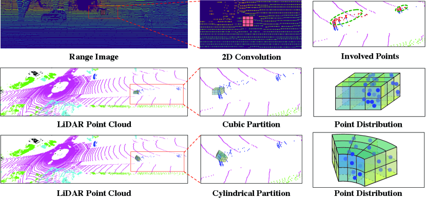
Recently, the advances in deep learning have significantly pushed forward the state of the art in image domain such as image segmentation and detection. Some existing LiDAR-based perception approaches follow this route to project the 3D point clouds onto a 2D space and process them via 2D convolution networks, including range image based [8, 10] and bird’s-eye-view image based [6, 11]. However, this group of methods lose and alter the accurate 3D geometric information during the 3D-to-2D projection (as shown in the top row of Fig. 1(a)).
A natural alternative is to utilize the 3D partition and 3D convolution networks to process the point cloud and maintain their 3D geometric relations. However, in our initial attempts, we directly apply the 3D voxelization [12, 13] and 3D convolution networks to outdoor LiDAR point cloud, only to find very limited performance gain (as shown in Fig. 1(b)). Our investigation into this issue reveals a key difficulty of outdoor LiDAR point cloud, namely sparsity and varying density, which is also the key difference to indoor scenes with dense and uniform-density points. However, previous 3D voxelization methods consider the point cloud as a uniform one and split them via the uniform cube, while neglecting the varying-density property of outdoor point cloud. Consequently, this effect to apply the 3D partition to outdoor point cloud is met with fundamental difficulty.
Motivated by these findings, we propose a new framework to outdoor LiDAR segmentation that consists of two key components, i.e., 3D cylindrical partition and asymmetrical 3D convolution networks, which maintain the 3D geometric information and handle these issues from partition and networks, respectively. Here, cylindrical partition resorts to the cylinder coordinates to divide the point cloud dynamically according to the distance (Regions that are far away from the origin have much sparse points, thus requiring a larger cell), which produces a more balanced point distribution (as shown in Fig. 1(a)); while asymmetrical 3D convolution networks strengthen the horizontal and vertical kernels to match the point distribution of objects in the driving scene and enhance the robustness to the sparsity. Moreover, voxel based methods might divide the points with different categories into the same cell and cell label encoding would inevitably cause the information loss (for LiDAR-based segmentation tasks). To alleviate the interference of lossy label encoding, a point-wise module is introduced to further refine the features obtained from voxel-based network. Overall, the cooperation of these components well maintains the geometric relation and tackle the difficulty of outdoor point cloud, thus improving the effectiveness of 3D frameworks.
Since the learned features from our model can be used for downstream tasks, we benchmark our model on a variety of LiDAR-based perception tasks such LiDAR-based semantic segmentation, panoptic segmentation and 3D detection. For semantic segmentation, we evaluate the proposed method on several large-scale outdoor datasets, including SemanticKITTI [14], nuScenes [15] and A2D2 [16]. Our method achieves the state-of-the-art on the leaderboard of SemanticKITTI (both single-scan and multi-scan challenges) and also outperforms the existing methods on nuScenes and A2D2 with a large margin. We also extend the proposed cylindrical partition and asymmetrical 3D convolution networks to LiDAR panoptic segmentation and LiDAR 3D detection. For panoptic segmentation and 3D detection, experimental results on SemanticKITTI and nuScenes, respectively, show its strong performance and good generalization capability.
The contributions of this work mainly lie in three aspects:
-
(1)
We reposition the focus of outdoor LiDAR segmentation from 2D projection to 3D structure, and further investigate the inherent properties (difficulties) of outdoor point cloud.
-
(2)
We introduce a new framework to explore the 3D geometric pattern and tackle these difficulties caused by sparsity and varying density, through cylindrical partition and asymmetrical 3D convolution networks.
-
(3)
The proposed method achieves the state of art on LiDAR-based semantic segmentation, LiDAR panoptic segmentation and LiDAR point cloud 3D detection, which also demonstrates its strong generalization capability.
2 Related Work
Deep Learning for Indoor-scene Point Cloud. Indoor-scene point clouds carry out some properties, including generally uniform density, small number of points, and small range of the scene. Mainstream methods [17, 18, 19, 20, 21, 22, 23, 24, 25, 26, 27, 28] of indoor point cloud segmentation learn the point features based on the raw point directly, which are often based on the pioneering work, i.e., PointNet, and promote the effectiveness of sampling, grouping and ordering to achieve the better performance. Another group of methods utilize the clustering algorithm [20, 21] to extract the hierarchical point features. However, these methods focusing on indoor point cloud are limited to adapt to the outdoor point cloud under the property of varying density and large range of scenes, and the large number of points also result in the computational difficulties for these methods when deploying from indoor to outdoor.
Deep Learning for Outdoor-scene Point Cloud. Most existing approaches for outdoor-scene point cloud [7, 29, 30, 8, 31, 32, 33, 34, 35] focus on converting the 3D point cloud to 2D grids, to enable the usage of 2D Convolutional Neural Networks. SqueezeSeg [10], Darknet [14], SqueezeSegv2 [36], and RangeNet++ [8] utilize the spherical projection mechanism, which converts the point cloud to a frontal-view image or a range image, and adopt the 2D convolution network on the pseudo image for point cloud segmentation or detection task. PolarNet [6] follows the bird’s-eye-view projection, which projects point cloud data into bird’s-eye-view representation under the polar coordinates. However, these 3D-to-2D projection methods inevitably loss and alter the 3D topology and fails to model the geometric information. Moreover, in most outdoor scenes, LiDAR device is often used to produce the point cloud data, where its inherent properties, i.e., sparsity and varying density , are often neglected.
3D Voxel Partition. 3D voxel partition is another routine of point cloud encoding [37, 38, 12, 13, 39, 40, 41]. It converts a point cloud into 3D voxels, which mainly retains the 3D geometric information. OccuSeg [37], SSCN [12] and SEGCloud [38] follow this line to utilize the voxel partition and apply regular 3D convolutions for LiDAR segmentation. It is worth noting that while the aforementioned efforts have shown encouraging results, the improvement in the outdoor LiDAR point cloud remains limited. As mentioned above, a common issue is that these methods neglect the inherent properties of outdoor LiDAR point cloud, namely, sparsity and varying density. Compared to these methods, our proposed method resorts to the 3D cylindrical partition and asymmetrical 3D convolution networks to tackle these difficulties.
Network Architectures for Feature Extraction . Fully Convolutional Network [42] is the fundamental work for segmentation tasks in the deep-learning era. Built upon the FCN, many works aim to improve the performance via exploring the dilated convolution, multi-scale context modeling and attention modeling, including DeepLab[43, 44] and PSP [45]. Recent work utilizes the neural architecture search to find the more effective backbone for the segmentation [46, 47]. Particularly, U-Net [48] proposes a symmetric architecture to incorporate the low-level features. With the great success of U-Net on 2D benchmarks and its good flexibility , many studies for LiDAR-based perception often adapt the U-Net to the 3D space [13]. We also follow this structure to construct our asymmetrical 3D convolution networks.
3 Methodology
3.1 Framework Overview
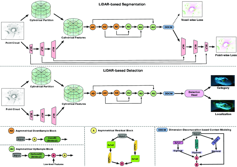
As shown in the top and middle row of Fig. 2, we elaborate the pipeline of our model in LiDAR-based segmentation and detection task. In the context of semantic segmentation, given a point cloud, the task is to assign the semantic label to each point. Based on the comparison between 2D and 3D representation and investigation of the inherent properties of outdoor LiDAR point cloud, we desire to obtain a framework which explores the 3D geometric information and handles the difficulty caused by sparsity and varying-density. To this end, we propose a new outdoor segmentation approach based on the 3D partition and 3D convolution networks. To handle these difficulties of outdoor LiDAR point cloud, namely sparsity and varying density, we first employ the cylindrical partition to generate the more balanced point distribution (more robust to varying density), then apply the asymmetrical 3D convolution networks to power the horizontal and vertical weights, thus well matching the object point distribution in driving scene and enhancing the robustness to the sparsity. Same backbone with cylindrical partition and asymmetrical convolution network is also adapted to LiDAR-based 3D detection (shown in the middle row of Fig. 2).
Specifically, the framework consists of two major components, including cylindrical partition and asymmetrical 3D convolution networks. The LiDAR point cloud is first divided by the cylindrical partition and the features extracted from MLP is then reassigned based on this partition. Asymmetrical 3D convolution networks are then used to generate the voxel-wise outputs. For segmentation tasks, a point-wise module is introduced to alleviate the interference of lossy cell-label encoding, thus refining the outputs. In the following sections, we will present these components in detail.
3.2 Cylindrical Partition
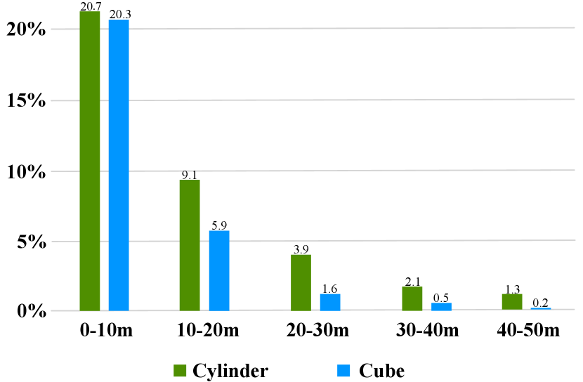
As mentioned above, outdoor-scene LiDAR point cloud possesses the property of varying density, where nearby region has much greater density than farther-away region. Therefore, uniform cells splitting the varying-density points would fall into an imbalanced distribution (for example, larger proportion of empty cells). While in the cylinder coordinate system, it utilizes the increasing grid size to cover the farther-away region, and thus more evenly distributes the points across different regions and gives an more balanced representation against the varying density. We perform a statistic to show the proportion of non-empty cells across different distances in Fig. 3. It can be found that with the distance goes far, cylindrical partition maintains a balanced non-empty proportion due to the increasing grid size while cubic partition suffers the imbalanced distribution, especially in the farther-away regions (about 6 times less than cylindrical partition). Moreover, unlike these projection-based methods project the point to the 2D view, cylindrical partition maintains the 3D grid representation to retain the geometric structure.
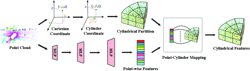
The workflow is illustrated in Fig. 4. We first transform the points on Cartesian coordinate system to the Cylinder coordinate system. This step transforms the points () to points (), where radius (distance to origin in x-y axis) and azimuth (angle from x-axis to y-axis) are calculated. Then cylindrical partition performs the split on these three dimensions, note that in the cylinder coordinate, the farther-away the region is, the larger the cell will be. Point-wise features obtained from the MLP are reassigned based on the result of this partition to get the cylindrical features. Specifically, the point-cylinder mapping contains the index of point-wise features to cylinder. Based on this mapping function, point-wise features within same cylinder are mapped together and processed via max-pooling to get the cylindrical features. After these steps, we unroll the cylinder from 0-degree and get the 3D cylindrical representation , where denotes the feature dimension and mean the radius, azimuth and height. Subsequent asymmetrical 3D convolution networks will be performing on this representation.
3.3 Asymmetrical 3D Convolution Network
Since the driving-scene point cloud carries out the specific object shape distribution, including car, truck, bus, motorcycle and other cubic objects, we aim to follow this observation to enhance the representational power of a standard 3D convolution. Moreover, recent literature [49, 50] also shows that the central crisscross weights count more in the square convolution kernel. In this way, we devise the asymmetrical residual block to strengthen the horizontal and vertical responses and match the object point distribution. Based on the proposed asymmetrical residual block, we further build the asymmetrical downsample block and asymmetrical upsample block to perform the downsample and upsample operation. Moreover, a dimension-decomposition based context modeling (termed as DDCM) is introduced to explore the high-rank global context in decomposite-aggregate strategy. We detail these components in the bottom of Fig. 2
Asymmetrical Residual Block Motivated by the observation and conclusion in [49, 50], the asymmetrical residual block strengthens the horizontal and vertical kernels, which matches the point distribution of object in the driving scene and explicitly makes the skeleton of the kernel powerful, thus enhancing the robustness to the sparsity of outdoor LiDAR point cloud. We use the Car and Motorcycle as the example to show the asymmetrical residual block in Fig. 6, where 3D convolutions are performing on the cylindrical grids. Moreover, the proposed asymmetrical residual block also saves the computation and memory cost compared to the regular square-kernel 3D convolution block. By incorporating the asymmetrical residual block, the asymmetrical downsample block and upsample block are designed and our asymmetrical 3D convolution networks are built via stacking these downsample and upsample blocks.
Dimension-Decomposition based Context Modeling Since the global context features should be high-rank to have enough capacity to capture the large context varieties [51], it is hard to construct these features directly. We follow the tensor decomposition theory [52] to build the high-rank context as a combination of low-rank tensors, where we use three rank-1 kernels to obtain the low-rank features and then aggregate them together to get the final global context.
3.4 Sparse Activation Visualization
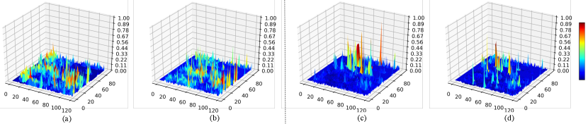
As mentioned above, the proposed cylindrical partition and asymmetrical 3D networks aim to tackle the difficulties caused by sparsity and varying-density in outdoor point cloud. We thus visualize some filter activations from regular 3D convolution networks (with regular cubic partition) and asymmetrical 3D convolution networks (with cylindrical partition), respectively. The results are shown in Fig. 5. Fig. 5(a) and (b) are extracted from regular 3D convolution networks, which are activated at almost regions; While the proposed asymmetrical 3D convolution networks strengthen sparser activations and focus on them (as shown in Fig. 5(c) and (d)), they mainly focus on some certain regions. It demonstrates that the proposed model could adaptively handle the sparse point cloud input and focus on some certain regions.
3.5 Point-wise Refinement Module
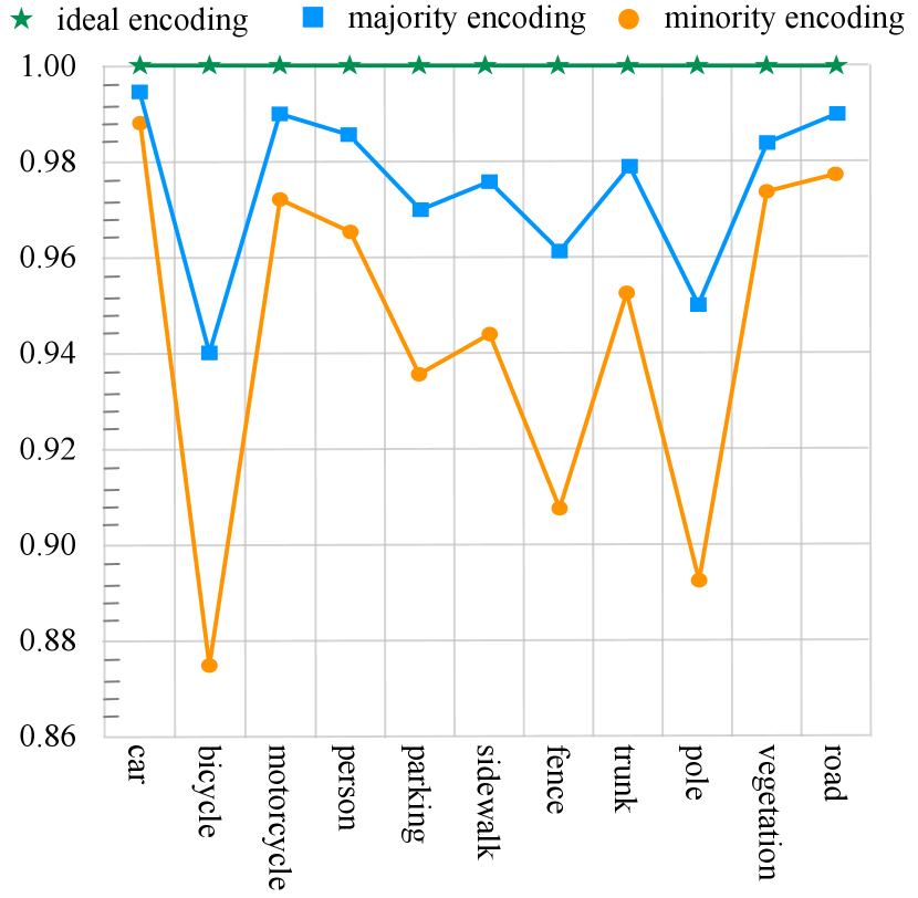
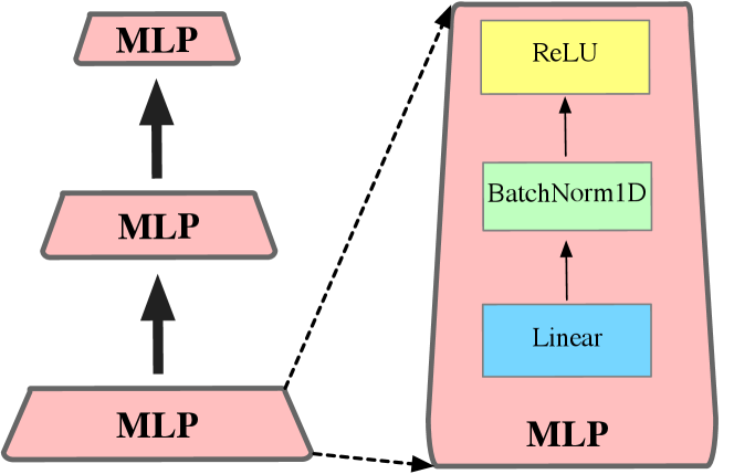
Partition-based methods predict one label for each cell. Although partition-based methods effectively explore the large-range point cloud, however, this group of method, including cube-based and cylinder-based, inevitably suffers from the lossy cell-label encoding, e.g., points with different categories are divided into same cell, and this case would cause the information loss for point cloud semantic segmentation task (as shown in the middle row of Fig. 2). We make a statistic to show the effect of different label encoding methods with cylindrical partition in Fig. 7, where majority encoding means using the major category of points inside a cell as the cell label and minority encoding indicates using the minor category as the cell label. It can be observed that both of them cannot reach the 100 percent mIoU (ideal encoding) and inevitably have the information loss. Here, the point-wise refinement module is introduced to alleviate the interference of lossy cell-label encoding. We first project the cylindrical features to the point-wise based on the inverse point-cylinder mapping table (note that points inside same cylinder would be assigned to the same cylindrical features). Then the point-wise module takes both point features before and after 3D convolution networks as the input, and fuses them together to refine the output. We also show the detailed structure of MLPs in point-wise refinement module and cylindrical partition in Fig. 8.
3.6 Objective Function
For LiDAR-based semantic segmentation task, the total objective of our method consists of two components, including voxel-wise loss and point-wise loss. It can be formulated as . For the voxel-wise loss (), we follow the existing methods [29, 7] and use the weighted cross-entropy loss and lovasz-softmax [53] loss to maximize the point accuracy and the intersection-over-union score, respectively. For point-wise loss (), we only use the weighted cross-entropy loss to supervise the training. During inference, the output from point-wise refinement module is used as the final output.
For LiDAR-based panoptic segmentation task, except the loss of semantic segmentation, it also contains the loss of instance branch [34], which utilizes center regression to achieve the clustering.
4 Experiments
In this section, we benchmark the proposed model on three downstream tasks. For semantic segmentation task, we evaluate the proposed method on several large-scale datasets, i.e., SemanticKITTI, nuScenes and A2D2. SemanticKITTI and nuScenes are also used in panoptic segmentation and 3D detection, respectively. Furthermore, extensive ablation studies on LiDAR semantic segmentation task are conducted to validate each component.
Methods mIoU car bicycle motorcycle truck other-vehicle person bicyclist motorcyclist road parking sidewalk other-ground building fence vegetation trunk terrain pole traffic TangentConv [56] 35.9 86.8 1.3 12.7 11.6 10.2 17.1 20.2 0.5 82.9 15.2 61.7 9.0 82.8 44.2 75.5 42.5 55.5 30.2 22.2 Darknet53 [14] 49.9 86.4 24.5 32.7 25.5 22.6 36.2 33.6 4.7 91.8 64.8 74.6 27.9 84.1 55.0 78.3 50.1 64.0 38.9 52.2 RandLA-Net [7] 50.3 94.0 19.8 21.4 42.7 38.7 47.5 48.8 4.6 90.4 56.9 67.9 15.5 81.1 49.7 78.3 60.3 59.0 44.2 38.1 RangeNet++ [8] 52.2 91.4 25.7 34.4 25.7 23.0 38.3 38.8 4.8 91.8 65.0 75.2 27.8 87.4 58.6 80.5 55.1 64.6 47.9 55.9 PolarNet [6] 54.3 93.8 40.3 30.1 22.9 28.5 43.2 40.2 5.6 90.8 61.7 74.4 21.7 90.0 61.3 84.0 65.5 67.8 51.8 57.5 SqueezeSegv3 [9] 55.9 92.5 38.7 36.5 29.6 33.0 45.6 46.2 20.1 91.7 63.4 74.8 26.4 89.0 59.4 82.0 58.7 65.4 49.6 58.9 Salsanext [29] 59.5 91.9 48.3 38.6 38.9 31.9 60.2 59.0 19.4 91.7 63.7 75.8 29.1 90.2 64.2 81.8 63.6 66.5 54.3 62.1 KPConv [18] 58.8 96.0 32.0 42.5 33.4 44.3 61.5 61.6 11.8 88.8 61.3 72.7 31.6 95.0 64.2 84.8 69.2 69.1 56.4 47.4 FusionNet [32] 61.3 95.3 47.5 37.7 41.8 34.5 59.5 56.8 11.9 91.8 68.8 77.1 30.8 92.5 69.4 84.5 69.8 68.5 60.4 66.5 KPRNet [57] 63.1 95.5 54.1 47.9 23.6 42.6 65.9 65.0 16.5 93.2 73.9 80.6 30.2 91.7 68.4 85.7 69.8 71.2 58.7 64.1 TORANDONet [58] 63.1 94.2 55.7 48.1 40.0 38.2 63.6 60.1 34.9 89.7 66.3 74.5 28.7 91.3 65.6 85.6 67.0 71.5 58.0 65.9 SPVNAS [47] 66.4 - - - - - - - - - - - - - - - - - - - Ours 67.8 97.1 67.6 64.0 59.0 58.6 73.9 67.9 36.0 91.4 65.1 75.5 32.3 91.0 66.5 85.4 71.8 68.5 62.6 65.6
Methods mIoU barrier bicycle bus car construction motorcycle pedestrian traffic-cone trailer truck driveable other sidewalk terrain manmade vegetation RangeNet++ [8] 65.5 66.0 21.3 77.2 80.9 30.2 66.8 69.6 52.1 54.2 72.3 94.1 66.6 63.5 70.1 83.1 79.8 PolarNet [6] 71.0 74.7 28.2 85.3 90.9 35.1 77.5 71.3 58.8 57.4 76.1 96.5 71.1 74.7 74.0 87.3 85.7 Salsanext [29] 72.2 74.8 34.1 85.9 88.4 42.2 72.4 72.2 63.1 61.3 76.5 96.0 70.8 71.2 71.5 86.7 84.4 Ours 76.1 76.4 40.3 91.2 93.8 51.3 78.0 78.9 64.9 62.1 84.4 96.8 71.6 76.4 75.4 90.5 87.4
4.1 Dataset and Metric
SemanticKITTI [14] is a large-scale driving-scene dataset for point cloud segmentation, including semantic segmentation and panoptic segmentation. It is derived from the KITTI Vision Odometry Benchmark and collected in Germany with the Velodyne-HDLE64 LiDAR. The dataset consists of 22 sequences, splitting sequences 00 to 10 as training set (where sequence 08 is used as the validation set), and sequences 11 to 21 as test set. 19 classes are remained for training and evaluation after merging classes with different moving status and ignore classes with very few points. In this dataset, it consists of two challenges, namely, single-scan and multi-scan point-cloud semantic segmentation, where single-scan denotes the single-frame point cloud semantic segmentation and multi-scan denotes the multiple-frame point cloud segmentation, respectively. The key difference is that multi-scan semantic segmentation requires classifying the moving categories, including moving car, moving truck, moving person, moving bicyclist, moving motorcyclist.
nuScenes [15] It collects 1000 scenes of 20s duration with 32 beams LiDAR sensor. The number of total frames is 40,000, which is sampled at 20Hz. They also officially split the data into training and validation set. After merging similar classes and removing rare classes, total 16 classes for the LiDAR semantic segmentation are remained.
A2D2 [16] We follow the data pre-processing in [6] to generate the label and process the point cloud data. A2D2 uses five asynchronous LiDAR sensors where each sensor covers a potion of the surrounding view. After LiDAR panoramic stitching, the A2D2 dataset is split into 22408, 2774 and 13264 training, validation and test scans, respectively with 38-class segmentation annotation. Since there are 38 categories in A2D2 dataset where some of them only have subtle differences, it is harder than other datasets, SemanticKITTI and nuScenes.
 |
 |
Implementation Details For these datasets, the Cartesian spaces are different which are related to the LiDAR sensor range. In our implementation, we fix the Cartesian spaces to be , , and for SemanticKITTI, nuScenes and A2D2, respectively. After transforming to the Cylindrical spaces, they are fixed to be , , and . In this way, the proposed cylindrical spaces can cover more than 99% of points for each point cloud scan on average and points out of the spaces are assigned to the closest cylindrical cell. For all datasets, cylindrical partition splits these point clouds into 3D representation with the size = , where three dimensions indicate the radius, angle and height, respectively. We also perform the ablation studies to investigate and cross-validate the effect of these parameters . We use NVIDIA V100 GPU with 16G memory to train the proposed model with batch size = 2.
Evaluation Metric To evaluate the proposed method, we follow the official guidance to leverage mean intersection-over-union (mIoU) as the evaluation metric defined in [14, 15], which can be formulated as: where represent true positive, false positive, and false negative predictions for class and the mIoU is the mean value of over all classes.
4.2 LiDAR-based Semantic Segmentation
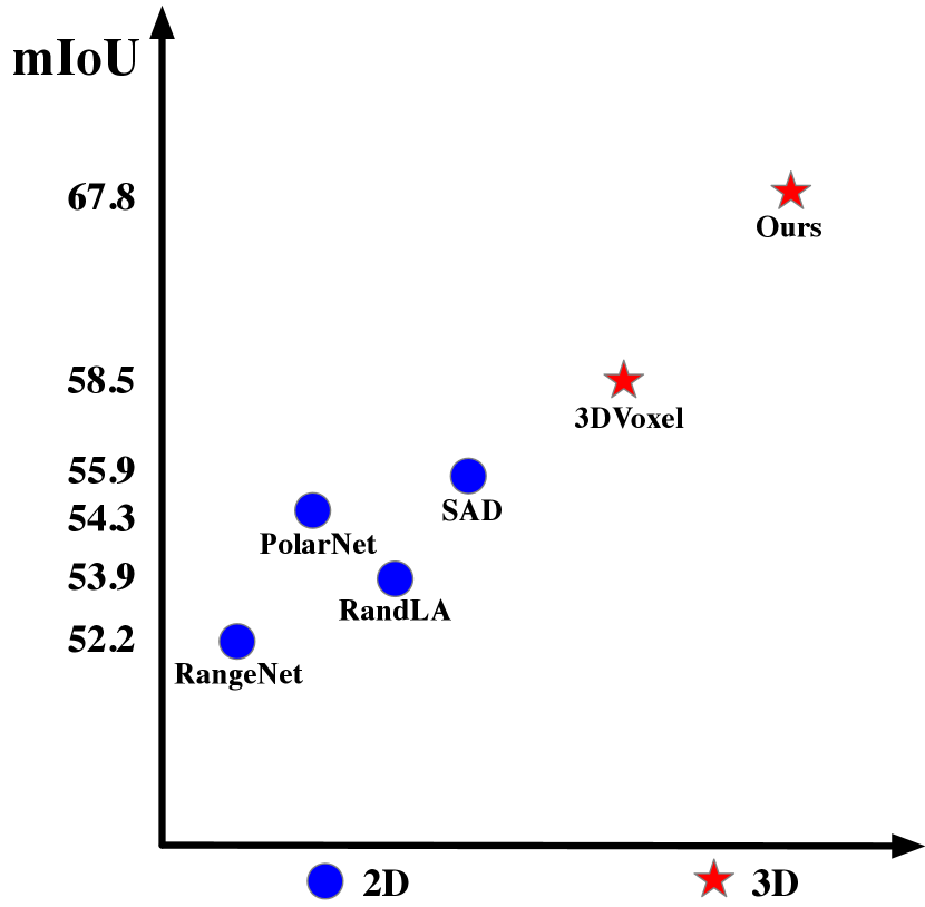
Results on SemanticKITTI Single-scan Semantic Segmentation In this experiment, we compare the results of our proposed method with existing state-of-the-art LiDAR segmentation methods on SemanticKITTI single-scan test set. The target is to generate the semantic prediction for single frame point cloud. As shown in Table I, our method outperforms all existing methods in term of mIoU. Compared to the projection-based methods on 2D space, including Darknet53 [14], SqueezeSegv3 [9], RangeNet++ [8] and PolarNet [6], our method achieves 8% 17% performance gain in term of mIoU due to the modeling of 3D geometric information. Compared to some voxel partition and 3D convolution based methods, including FusionNet [32], TORANDONet [58] (multi-view fusion based method) and SPVNAS [47] (utilizing the neural architecture search for LiDAR segmentation), the proposed method also performs better than these 3D convolution based methods, where the cylindrical partition and asymmetrical 3D convolution networks well handle the difficulty of driving-scene LiDAR point cloud that is neglected by these methods.
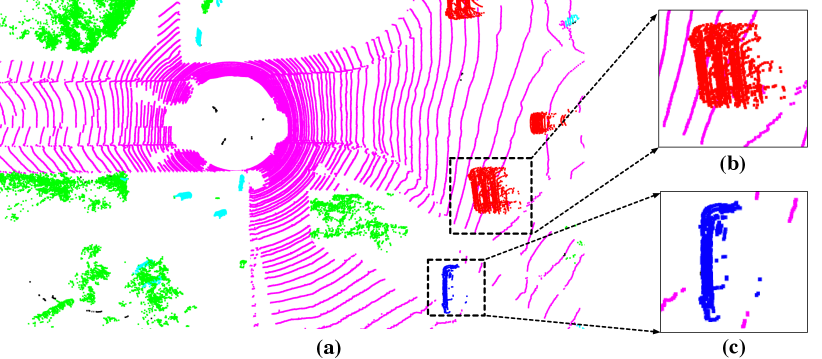
Visualization We show some visualization results of single-scan segmentation in Fig.9, which are sampled from the SemanticKITTI validation set. It can be observed that the proposed method mainly achieves decent accuracy, and well separates the nearby objects and accurately identifies them because it maintains the 3D topology and utilizes the geometric information (we highlight corresponding regions with red rectangles). These visualization can verify our claim that keeping 3D structure and more balanced point distribution could benefit the segmentation results.
Methods mIoU car bicycle motorcycle truck other-vehicle person bicyclist motorcyclist road parking sidewalk other-ground building fence TangentConv [56] 34.1 84.9 2.0 18.2 21.1 18.5 1.6 0.0 0.0 83.9 38.3 64.0 15.3 85.8 49.1 DarkNet53 [59] 41.6 84.1 30.4 32.9 20.0 20.7 7.5 0.0 0.0 91.6 64.9 75.3 27.5 85.2 56.5 SpSeqnet [60] 43.1 88.5 24.0 26.2 29.2 22.7 6.3 0.0 0.0 90.1 57.6 73.9 27.1 91.2 66.8 KPConv [18] 51.2 93.7 44.9 47.2 42.5 38.6 21.6 0.0 0.0 86.5 58.4 70.5 26.7 90.8 64.5 Ours 51.5 93.8 67.6 63.3 41.2 37.6 12.9 0.1 0.1 90.4 66.3 74.9 32.1 92.4 65.8
Methods mIoU vegetation trunk terrain pole traffic mov car mov truck moving other mov person mov biclist mov motorlist TangentConv [56] 34.1 79.5 43.2 56.7 36.4 31.2 40.3 1.1 6.4 1.9 30.1 42.2 DarkNet53 [59] 41.6 78.4 50.7 64.8 38.1 53.3 61.5 14.1 15.2 0.2 28.9 37.8 SpSeqnet [60] 43.1 84.0 66.0 65.7 50.8 48.7 53.2 41.2 26.2 36.2 2.3 0.1 KPConv [18] 51.2 84.6 70.3 66.0 57.0 53.9 69.4 0.5 0.5 67.5 67.4 47.2 Ours 51.5 85.4 72.8 68.1 62.6 61.3 68.1 0.0 0.1 63.1 60.0 0.4
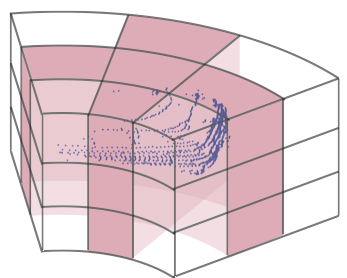
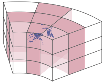
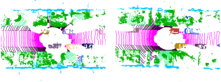
Results on SemanticKITTI Multi-scan Semantic Segmentation Unlike the single-scan semantic segmentation, the multi-scan segmentation in SemanticKITTI takes multiple frame point cloud as input and generates the more categories under moving status, including moving car, moving truck, moving other-vehicle, moving person, moving bicyclist and moving motorcyclist. In this experiment, we first perform the multiple-frame point cloud fusion. Specifically, the sequential point clouds in LiDAR coordinate are firstly transformed to global coordinate. Then, these sequential point clouds are fused in the global coordinate. Finally, all these points are transformed to the coordinate of last frame. In this way, we can achieve the multiple-frame fusion and we use 3 sequential point clouds as input data in our implementation. We show an example in Fig. 10. It can be found that moving cars have multiple shifting point clouds while stationary cars keep all points in same location.
The results of multi-scan semantic segmentation are shown in Table III and IV. Generally, our method outperforms all existing methods in terms of mIoU, where it achieves 0.3% and 8.4% gain compared to KPConv [18] (ICCV2019) and SpSeqnet [60] (CVPR2020), respectively. Our method obtains superior performance for most categories, even for some small objects, like bicycle and motorcycle, etc. For these moving categories, our method achieves the best performance on moving car and moving truck.
Results on nuScenes For nuScenes LiDARseg dataset, we report the results on its validation set. As shown in Table II, our method achieves better performance than existing methods in all categories, and this consistent performance improvement demonstrates the capability of the proposed model. Specifically, the proposed method obtains about 4% 7% performance gain than projection-based methods. Moreover, for these categories with sparse points, such as bicycle and pedestrian, our method significantly outperforms existing approaches, which also demonstrates the effectiveness of the proposed method to tackle the sparsity and varying density. Note that RangeNet++ [8] and Salsanext [29] perform the post-processing, including KNN, etc.
Methods mIoU car bicycle pedestrian truck small-vehi traffic-signal traffic-sign utility-vehi sidebars bumper curbstone solid line irrelevant signs road blocks tractor non-drivable zebra crossing Squeezeseg [10] 8.9 9.7 0.0 0.0 15.8 0.0 0.7 64.4 0.0 0.4 0.0 2.2 15.6 0.5 15.9 0.0 0.0 0.0 Squeezesegv2 [36] 16.4 15.4 0.2 8.6 63.8 0.0 16.8 61.7 0.6 0.1 0.0 14.8 24.7 12.7 33.2 0.0 5.8 0.0 DarkNet53 [59] 17.2 15.2 0.8 6.1 68.5 0.0 15.5 63.8 0.4 0.3 0.0 17.3 23.8 13.3 35.6 0.0 6.3 0.0 PolarNet [6] 23.9 23.8 10.1 18.2 69.7 9.6 49.1 58.5 0.0 11.3 0.0 28.3 37.6 24.8 42.8 0.0 14.8 0.0 Ours 27.1 20.1 21.1 29.6 77.8 26.7 58.6 67.6 4.6 10.3 0.0 33.4 43.9 29.9 51.0 0.0 19.9 0.0
Methods mIoU Obstacles Poles RD restricted area Animals Grid structure Signal corpus Drivable cobbleston Electronic traffic Slow drive area Nature object Parking area Sidewalk Ego car Painted driv instr Traffic guide obj Dashed line RD normal street Sky Buildings Blurred area Rain dirt Squeezeseg [10] 8.9 0.0 0.3 0.0 0.0 0.0 0.0 0.0 0.0 0.0 64.5 0.0 13.7 0.0 0.0 0.1 0.2 77.7 10.4 27.7 0.0 0.0 Squeezesegv2 [36] 16.4 0.2 5.2 29.5 0.0 10.3 5.5 2.7 0.0 1.9 76.4 3.8 29.2 0.0 6.4 12.4 17.1 85.8 12.1 50.9 0.0 0.0 DarkNet53 [59] 17.2 3.9 7.6 38.7 0.0 10.8 4.4 3.3 0.0 0.0 77.9 3.1 31.5 0.0 9.4 7.3 15.7 86.4 12.9 55.2 0.0 0.0 PolarNet [6] 23.9 8.0 11.0 55.6 0.0 14.8 11.9 7.0 0.0 4.4 81.6 12.8 42.5 0.0 12.7 11.5 31.8 90.3 9.2 57.0 0.0 0.0 Ours 27.1 15.6 14.0 60.8 0.0 23.4 21.1 13.5 0.41 0.29 84.8 10.2 46.7 0.0 20.0 23.8 34.6 91.3 10.0 64.0 0.0 0.0
Results on A2D2 We report the results on A2D2 [16] validation set. As shown in Table V and VI, it can be observed that the proposed method performs much better than existing methods about 3% in terms of mIoU, including Squeezeseg [10], SqueezesegV2 [36], DarkNet53 [59] and PolarNet [6], where all of them are based on the 2D projection and 2D convolution networks. Specifically, our method achieves better performance on almost all categories consistently, which also demonstrates the effectiveness of our method. Note that due to the more fine-grained categories in A2D2 (38 categories in total), it is harder than other datasets, such as SemanticKITTI and nuScenes, and there exist more categories with zero values.
In general, our method achieves the consistent state-of-the-art performance in all three datasets with different settings (single-scan and multi-scan) and sensor ranges. It clearly demonstrates the effectiveness of the proposed method and its good generalization capability across different datasets.
4.3 LiDAR-based Panoptic Segmentation
Panoptic segmentation is first proposed in [61] as a new task, in which semantic segmentation is performed for background classes and instance segmentation for foreground classes and these two groups of category are also termed as stuff and things classes, respectively. Behley et al. [62] extend the task to LiDAR point clouds and propose the LiDAR panoptic segmentation. In this experiment, we conduct the panoptic segmentation on SemanticKITTI dataset and report results on the validation set. For the evaluation metrics, we follow the metrics defined in [62], where they are the same as that of image panoptic segmentation defined in [61] including Panoptic Quality (PQ), Segmentation Quality (SQ) and Recognition Quality (RQ) which are calculated across all classes. PQ is defined by swapping PQ of each stuff class to its IoU and averaging over all classes like PQ does. Since the categories in panoptic segmentation contain two groups, i.e., stuff and things, these metrics are also performed separately on these two groups, including PQTh, PQSt, RQTh, RQSt, SQTh and SQSt, where Panoptic Quality (PQ) is usually used as the first criteria. For the experimental setting, we follow the LiDAR semantic segmentation, where Adam optimizer with learning rate = is used for optimization.
In this experiment, we use the proposed cylindrical partition as the partition method and asymmetrical 3D convolution networks as the backbone. Moreover, a semantic branch is used to output the semantic labels for stuff categories, and an instance branch is introduced to generate the instance-level features and further extract their instance IDs for things categories through heuristic clustering algorithms (we use mean-shift in the implementation and the bandwidth of the Mean Shift used in our backbone method is set to while the minimum number of points in a valid instance is set to 50 for SemanticKITTI).
We report the results in Table VII. It can be found that our method achieves much better performance than existing methods [63, 64]. In terms of PQ, we have about 4.7% point improvement, and particularly for the thing categories, our method significantly outperforms state-of-the-art in terms of PQTh and RQTh with a large margin of 10% points. It indicates that our cylindrical partition and asymmetrical 3D convolution networks significantly benefit the recognition of the things classes. It is worthy of noting that PointGroup and LPASD perform poorly on the outdoor LiDAR segmentation task which indicates that these indoor methods are not suitable for the challenging outdoor point clouds due to the different scenarios and inherent properties. Experimental results demonstrate the effectiveness of the proposed method and its good generalization ability. We show several samples of panoptic segmentation results in Fig. 11, where different colors represent different vehicles.
| Method | PQ | PQ | RQ | SQ | PQTh | RQTh | SQTh | PQSt | RQSt | SQSt | mIoU |
| KPConv [18] + PV-RCNN [65] | 51.7 | 57.4 | 63.1 | 78.9 | 46.8 | 56.8 | 81.5 | 55.2 | 67.8 | 77.1 | 63.1 |
| PointGroup [64] | 46.1 | 54.0 | 56.6 | 74.6 | 47.7 | 55.9 | 73.8 | 45.0 | 57.1 | 75.1 | 55.7 |
| LPASD [63] | 36.5 | 46.1 | - | - | - | 28.2 | - | - | - | - | 50.7 |
| Ours | 56.4 | 62.0 | 67.1 | 76.5 | 58.8 | 66.8 | 75.8 | 54.8 | 67.4 | 77.1 | 63.5 |
| Methods | mAP | NDS |
|---|---|---|
| PointPillar [11] | 30.5 | 45.3 |
| PP + Reconfig [66] | 32.5 | 50.6 |
| SECOND [55] | 31.6 | 46.8 |
| SECOND [55] + Cylinder | 34.3 | 49.6 |
| SECOND [55] + Asym-CNN | 33.0 | 48.3 |
| SECOND [55] + CyAs | 36.4 | 51.7 |
| SSN [54] | 46.3 | 56.9 |
| SSN [54] + CyAs | 47.7 | 58.2 |
| SSNv2 [54]⋆ | 50.6 | 61.6 |
| SSNv2 [54]⋆ + CyAs | 52.8 | 64.0 |
4.4 LiDAR-based 3D Detection
LiDAR 3D detection aims to localize and classify the multi-class objects in the point cloud. SECOND [55] first utilizes the 3D voxelization and 3D convolution networks to perform the single-stage 3D detection. In this experiment, we follow SECOND method and replace the regular voxelization and 3D convolution with the proposed cylindrical partition and asymmetrical 3D convolution networks, respectively. Similarly, to verify its scalability, we also extend the proposed modules to SSN [54]. Furthermore, another strong baseline, SSNv2 [54], is also adapted to verify the effectiveness of our method when the baseline is very competitive. The experiments are conducted on nuScenes dataset and the cylindrical partition also generates the representation. For the evaluation metrics, we follow the official metrics defined in nuScenes, i.e., mean average precision (mAP) and nuScenes detection score (NDS). For other experimental settings, including the optimization method, target assignment, anchor size and network architecture of multiple heads, we all follow the setting in SSN [54].
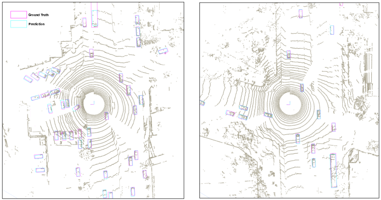
The results are shown in Table VIII. PP + Reconfig [66] is a partition enhancement approach based on PointPillar [11], while our SECOND + CyAs performs better with similar backbone, which indicates the superiority of the cylindrical partition. To verify the effect of different components (i.e., Cylinder partition and Asymmetrical 3D convolution networks) of our method on LiDAR 3D detection, we design two variants, i.e., SECOND [55] + Cylinder and SECOND [55] + Asym-CNN. The results shown in Table VIII demonstrate that these two components in our method consistently improve the baseline method with 2.8% points and 1.5% points in terms of NDS, respectively. We then extend the proposed method (i.e., CyAs) to two baseline methods, termed as SECOND + CyAs and SSN + CyAs, respectively. By comparing these two models with their extensions, it can be observed that the proposed Cylindrical partition and Asymmetrical 3D convolution networks boost the performance consistently, even for the strong baseline i.e., SSNv2, which demonstrates the effectiveness and scalability of our model. For different backbones, like SECOND and SSN, our method could consistently benefit them, showing its good generalization ability. Several qualitative results on nuScenes dataset are shown in Fig. 12.
4.5 Ablation Studies
In this section, we perform the thorough ablation experiments on LiDAR-based semantic segmentation task to investigate the effect of different components in our method. We also design several variants of asymmetrical residual block to verify our claim that strengthening the horizontal and vertical kernels power the representation ability for driving-scene point cloud. For the 3D representation after cylindrical partition, we also try several other hyper-parameters to cross-validate these values.
| Baseline | Cylinder | Asym-CNN | DDCM | PR | mIoU |
|---|---|---|---|---|---|
| ✓ | 58.1 | ||||
| ✓ | ✓ | 61.0 | |||
| ✓ | ✓ | ✓ | 63.8 | ||
| ✓ | ✓ | ✓ | ✓ | 65.2 | |
| ✓ | ✓ | ✓ | ✓ | ✓ | 65.9 |
Effects of Network Components In this part, we make several variants of our model to validate the contributions of different components. The results on SemanticKITTI validation set are reported in Table IX. Baseline method denotes the framework using 3D voxel partition (with cubic partition) and 3D convolution networks. It can be observed that cylindrical partition performs much better than cubic-based partition with about 3% mIoU gain and asymmetrical 3D convolution networks also significantly boost the performance about 3% improvement, which demonstrates that both cylindrical partition and asymmetrical 3D convolution networks are crucial in the proposed method. Furthermore, dimension-decomposition based context modeling delivers the effective global context features, which yields an improvement of 1.4%. Point-wise refinement module further pushes forward the performance based on the strong model, about 0.7%. Generally, the proposed cylindrical partition and asymmetrical 3D convolution networks make the most contribution to the performance improvement.
Methods mIoU car bicycle motorcycle truck other-vehicle person bicyclist motorcyclist road parking sidewalk other-ground building fence vegetation trunk terrain pole traffic Regular 60.8 96.7 43.5 50.6 78.0 56.4 64.5 81.7 0.1 93.5 38.2 78.6 0.2 89.5 54.0 86.9 61.4 71.8 62.8 46.2 1D-asymmetrical 61.9 96.7 44.3 56.4 83.2 60.6 64.8 89.9 2.3 93.1 36.2 78.0 0.4 88.5 49.5 86.7 64.8 70.6 63.3 48.7 Asymmetrical(ours) 63.9 96.8 54.4 76.1 80.1 65.3 74.2 88.7 6.2 90.1 36.6 75.1 0.4 83.3 55.2 86.4 67.3 67.1 63.4 46.7
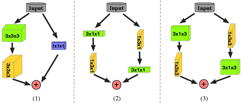
Variants of Asymmetrical Residual Block To verify the effectiveness of the proposed asymmetrical residual block, we design several variants of asymmetrical residual block to investigate the effect of horizontal and vertical kernel enhancement (as shown in Fig. 13). The first variant is the regular residual block without any asymmetrical structure. The second one is the 1D-asymmetrical residual block, which utilizes the 1D asymmetrical kernels without height and also strengthens the horizontal or vertical kernels in one-dimension. The third one is the proposed asymmetrical residual block, which strengthens both horizontal and vertical kernels. These variants strengthen the skeleton of convolution kernels step by step (from regular residual block to asymmetrical kernel without height, then to both horizontal and vertical kernels with height).
We conduct the ablation studies on SemanticKITTI validation set. Note that we use the cylindrical partition as the partition method and stack these proposed variants to build the 3D convolution networks for this ablation experiment. We report the results in Table X. It can be found that although the 1D-Asymmetrical residual block only powers the horizontal and vertical kernels in one-dimension, it still achieves 1.3% gain in terms of mIoU and it obtains about more than 5% performance gain for motorcycle, other-vehicle and bicyclist, which demonstrates the effectiveness of strengthening skeleton of convolution kernel, even without height dimension. After taking the height into the consideration, the proposed asymmetrical residual block further matches the object distribution in driving scene and powers the skeleton of kernels, which enhances the robustness to the sparsity. From Table X, the proposed asymmetrical residual block significantly boosts the performance with about 3% improvements, where large improvement can be observed on some instance categories (about 10% gain), including bicycle, person, other-vehicle and motorcycle, because it matches the point distribution of object and enhances the representational power.
Size of 3D Representation As mentioned in implementation details, we set the size of 3D representation to . In this experiment, we use other hyper-parameters to cross-validate these values, including and . They cover the denser and sparser representations compared with representation. Furthermore, we also introduce a cubic partition with size of as the counterpart to investigate the effectiveness and compactness of cylindrical partition.
We conduct the experiments on SemanticKITTI validation set and all experiments are under same settings except the different representation size. The results are shown in Table XI. It can be found that the 3D representation with performs better than other two representations with 2% point improvement than and . Since representation delivers compacter representation with larger cylindrical cells, it however might mis-split the points across different categories into same cell, which inevitably increases the information loss; While for representation, it contains fine-grained cylindrical cell, but generates the larger representation, which might burden the training of 3D convolution and cause the degradation of performance. Compared to the cubic partition with , all cylindrical partitions achieve much better performance and this consistent performance gain demonstrates its effectiveness. From this experiment, we cross-validate the representation and investigate the effect of different size of 3D representations.
| Size of Representation | mIoU |
|---|---|
| (cubic) | 58.1 |
| 63.4 | |
| 64.1 | |
| 65.9 |
5 Discussion
5.1 Comparison of Inference Time
| Methods | Latency (ms) | mIoU(%) |
|---|---|---|
| TangentConv [56] | 3000 | 40.9 |
| RandLA [7] | 800 | 53.9 |
| KPConv [18] | 263 | 58.8 |
| MinkowskiNet [67] | 294 | 63.1 |
| SPVNAS-lite [47] | 110 | 63.7 |
| SPVNAS [47] | 259 | 66.4 |
| Ours | 170 | 67.8 |
To investigate the efficiency of the proposed method, we further make a statistic of inference time compared to existing methods. In the experiment, we keep the setting unchanged and set the mode as the evaluation mode to calculate the inference time. The results of inference time of existing methods are directly token from [59].
The results are shown in Table XII. Compared to 2D projection based method (inference time consists of computation time and post-processing time), i.e., RandLA [7], our method achieves about 5.0 speedup with 14% performance improvement due to no requirement for post-processing. Moreover, compared to other 3D based methods, including MinkowskiNet [67] and SPVNAS [47], we also achieve the better performance and less inference time. The main reasons lie in two aspects: 1) the proposed cylindrical partition generates compacter representation compared to regular cubic partition. For example, the regular cubic partition often has the cell of , and it thus generates a 3D representation of , which is more than 4 times larger than the cylindrical partition. 2) the asymmetrical 3D convolution networks consume smaller computational overhead and less parameters compared to the regular 3D convolution networks. Specifically, using a convolution with kernel= followed by a convolution is equivalent to sliding a two layer network with the same receptive field as in a 3D convolution with kernel= , but it has 33% cheaper computational cost than a convolution with same number of output filters. The corporation of these two parts leads to the effective and efficient approach.
5.2 Comparison with other methods dealing with sparsity issue
Our proposed method utilizes the cylindrical partition and asymmetrical 3D convolution networks to handle the inherent difficulties, i.e., sparsity and varying density. Hence, we further compare the proposed method with other methods tackling the sparsity issue, to verify its effectiveness. Specifically, SPVNAS [47] proposes a sparse point-voxel convolution to preserve the fine details and deal with sparsity. MinkowskiNet [67] adopts sparse tensors and proposes a generalized sparse convolution. We take them as the counterpart dealing with the sparsity issue and make a comparison with them. Note that in our implementation, we also use the sparse convolution [55] to build up the asymmetrical 3D convolution networks.
| Methods | SparseConv | Latency (ms) | mIoU(%) |
|---|---|---|---|
| MinkowskiNet [67] | ✓ | 294 | 63.1 |
| SPVNAS [47] | ✓ | 259 | 66.4 |
| Ours | ✓ | 170 | 67.8 |
The results are shown in Table XIII. Compared to other methods handling the sparsity issue, our method achieves both better performance and efficiency, which also demonstrates the superiority of our method.
6 Conclusion
In this paper, we have proposed a cylindrical and asymmetrical 3D convolution networks for LiDAR segmentation, where it maintains the 3D geometric relation. Specifically, two key components, the cylinder partition and asymmetrical 3D convolution networks, are designed to handle the inherent difficulties in outdoor LiDAR point cloud, namely sparsity and varying density, effectively and robustly. We conduct the extensive experiments and ablation studies, where the model achieves the state-of-the-art in SemanticKITTI, A2D2 and nuScenes, and keeps good generalization ability to other LiDAR based tasks, including LiDAR panoptic segmentation and LiDAR 3D detection.
References
- [1] Y. Ma, X. Zhu, S. Zhang, R. Yang, W. Wang, and D. Manocha, “Trafficpredict: Trajectory prediction for heterogeneous traffic-agents,” in Proceedings of the AAAI Conference on Artificial Intelligence, vol. 33, no. 01, 2019, pp. 6120–6127.
- [2] Y. Xu, X. Zhu, J. Shi, G. Zhang, H. Bao, and H. Li, “Depth completion from sparse lidar data with depth-normal constraints,” in Proceedings of the IEEE/CVF International Conference on Computer Vision, 2019, pp. 2811–2820.
- [3] T. Wang, X. Zhu, J. Pang, and D. Lin, “Probabilistic and geometric depth: Detecting objects in perspective,” arXiv preprint arXiv:2107.14160, 2021.
- [4] ——, “Fcos3d: Fully convolutional one-stage monocular 3d object detection,” arXiv preprint arXiv:2104.10956, 2021.
- [5] X. Peng, X. Zhu, T. Wang, and Y. Ma, “Side: Center-based stereo 3d detector with structure-aware instance depth estimation,” arXiv preprint arXiv:2108.09663, 2021.
- [6] Y. Zhang, Z. Zhou, P. David, X. Yue, Z. Xi, B. Gong, and H. Foroosh, “Polarnet: An improved grid representation for online lidar point clouds semantic segmentation,” in CVPR, 2020, pp. 9601–9610.
- [7] Q. Hu, B. Yang, L. Xie, S. Rosa, Y. Guo, Z. Wang, N. Trigoni, and A. Markham, “Randla-net: Efficient semantic segmentation of large-scale point clouds,” in CVPR, 2020, pp. 11 108–11 117.
- [8] A. Milioto, I. Vizzo, J. Behley, and C. Stachniss, “Rangenet++: Fast and accurate lidar semantic segmentation,” in IROS. IEEE, 2019, pp. 4213–4220.
- [9] C. Xu, B. Wu, Z. Wang, W. Zhan, P. Vajda, K. Keutzer, and M. Tomizuka, “Squeezesegv3: Spatially-adaptive convolution for efficient point-cloud segmentation,” arXiv preprint arXiv:2004.01803, 2020.
- [10] B. Wu, A. Wan, X. Yue, and K. Keutzer, “Squeezeseg: Convolutional neural nets with recurrent crf for real-time road-object segmentation from 3d lidar point cloud,” in ICRA. IEEE, 2018, pp. 1887–1893.
- [11] A. H. Lang, S. Vora, H. Caesar, L. Zhou, J. Yang, and O. Beijbom, “Pointpillars: Fast encoders for object detection from point clouds,” in CVPR, 2019, pp. 12 697–12 705.
- [12] B. Graham, M. Engelcke, and L. Van Der Maaten, “3d semantic segmentation with submanifold sparse convolutional networks,” in CVPR, 2018, pp. 9224–9232.
- [13] Ö. Çiçek, A. Abdulkadir, S. S. Lienkamp, T. Brox, and O. Ronneberger, “3d u-net: learning dense volumetric segmentation from sparse annotation,” in MICCAI. Springer, 2016, pp. 424–432.
- [14] J. Behley, M. Garbade, A. Milioto, J. Quenzel, S. Behnke, C. Stachniss, and J. Gall, “Semantickitti: A dataset for semantic scene understanding of lidar sequences,” in ICCV, 2019, pp. 9297–9307.
- [15] H. Caesar, V. Bankiti, A. H. Lang, S. Vora, V. E. Liong, Q. Xu, A. Krishnan, Y. Pan, G. Baldan, and O. Beijbom, “nuscenes: A multimodal dataset for autonomous driving,” arXiv preprint arXiv:1903.11027, 2019.
- [16] J. Geyer, Y. Kassahun, M. Mahmudi, X. Ricou, and R. Durgesh, “A2d2: Aev autonomous driving dataset,” Note: http://www. a2d2. audi, vol. 1, no. 4, 2019.
- [17] C. R. Qi, H. Su, K. Mo, and L. J. Guibas, “Pointnet: Deep learning on point sets for 3d classification and segmentation,” in CVPR, 2017, pp. 652–660.
- [18] H. Thomas, C. R. Qi, J.-E. Deschaud, B. Marcotegui, F. Goulette, and L. J. Guibas, “Kpconv: Flexible and deformable convolution for point clouds,” in ICCV, 2019, pp. 6411–6420.
- [19] W. Wu, Z. Qi, and L. Fuxin, “Pointconv: Deep convolutional networks on 3d point clouds,” in CVPR, 2019, pp. 9621–9630.
- [20] Y. Wang, Y. Sun, Z. Liu, S. E. Sarma, M. M. Bronstein, and J. M. Solomon, “Dynamic graph cnn for learning on point clouds,” Acm Transactions On Graphics (tog), vol. 38, no. 5, pp. 1–12, 2019.
- [21] P. Veličković, G. Cucurull, A. Casanova, A. Romero, P. Lio, and Y. Bengio, “Graph attention networks,” arXiv preprint arXiv:1710.10903, 2017.
- [22] Y. Lyu, X. Huang, and Z. Zhang, “Learning to segment 3d point clouds in 2d image space,” in CVPR, 2020, pp. 12 255–12 264.
- [23] F. Engelmann, M. Bokeloh, A. Fathi, B. Leibe, and M. Nießner, “3d-mpa: Multi-proposal aggregation for 3d semantic instance segmentation,” in CVPR, 2020, pp. 9031–9040.
- [24] J. Zhang, C. Zhu, L. Zheng, and K. Xu, “Fusion-aware point convolution for online semantic 3d scene segmentation,” in CVPR, 2020, pp. 4534–4543.
- [25] X. Yan, C. Zheng, Z. Li, S. Wang, and S. Cui, “Pointasnl: Robust point clouds processing using nonlocal neural networks with adaptive sampling,” in CVPR, 2020, pp. 5589–5598.
- [26] L. Wang, Y. Huang, Y. Hou, S. Zhang, and J. Shan, “Graph attention convolution for point cloud semantic segmentation,” in CVPR, 2019, pp. 10 296–10 305.
- [27] Q.-H. Pham, T. Nguyen, B.-S. Hua, G. Roig, and S.-K. Yeung, “Jsis3d: joint semantic-instance segmentation of 3d point clouds with multi-task pointwise networks and multi-value conditional random fields,” in CVPR, 2019, pp. 8827–8836.
- [28] X. Qi, R. Liao, J. Jia, S. Fidler, and R. Urtasun, “3d graph neural networks for rgbd semantic segmentation,” in ICCV, 2017, pp. 5199–5208.
- [29] T. Cortinhal, G. Tzelepis, and E. E. Aksoy, “Salsanext: Fast, uncertainty-aware semantic segmentation of lidar point clouds for autonomous driving,” 2020.
- [30] L. Zhao, H. Zhou, X. Zhu, X. Song, H. Li, and W. Tao, “Lif-seg: Lidar and camera image fusion for 3d lidar semantic segmentation,” arXiv preprint arXiv:2108.07511, 2021.
- [31] I. Alonso, L. Riazuelo, L. Montesano, and A. C. Murillo, “3d-mininet: Learning a 2d representation from point clouds for fast and efficient 3d lidar semantic segmentation,” arXiv preprint arXiv:2002.10893, 2020.
- [32] F. Zhang, J. Fang, B. Wah, and P. Torr, “Deep fusionnet for point cloud semantic segmentation,” ECCV, 2020.
- [33] L. Landrieu and M. Simonovsky, “Large-scale point cloud semantic segmentation with superpoint graphs,” in CVPR, 2018, pp. 4558–4567.
- [34] F. Hong, H. Zhou, X. Zhu, H. Li, and Z. Liu, “Lidar-based panoptic segmentation via dynamic shifting network,” arXiv preprint arXiv:2011.11964, 2020.
- [35] P. Cong, X. Zhu, and Y. Ma, “Input-output balanced framework for long-tailed lidar semantic segmentation,” in 2021 IEEE International Conference on Multimedia and Expo (ICME). IEEE, 2021, pp. 1–6.
- [36] B. Wu, X. Zhou, S. Zhao, X. Yue, and K. Keutzer, “Squeezesegv2: Improved model structure and unsupervised domain adaptation for road-object segmentation from a lidar point cloud,” in ICRA. IEEE, 2019, pp. 4376–4382.
- [37] L. Han, T. Zheng, L. Xu, and L. Fang, “Occuseg: Occupancy-aware 3d instance segmentation,” in CVPR, 2020, pp. 2940–2949.
- [38] L. Tchapmi, C. Choy, I. Armeni, J. Gwak, and S. Savarese, “Segcloud: Semantic segmentation of 3d point clouds,” in 3DV. IEEE, 2017, pp. 537–547.
- [39] H.-Y. Meng, L. Gao, Y.-K. Lai, and D. Manocha, “Vv-net: Voxel vae net with group convolutions for point cloud segmentation,” in ICCV, 2019, pp. 8500–8508.
- [40] H. Zhou, X. Zhu, X. Song, Y. Ma, Z. Wang, H. Li, and D. Lin, “Cylinder3d: An effective 3d framework for driving-scene lidar semantic segmentation,” arXiv preprint arXiv:2008.01550, 2020.
- [41] X. Zhu, H. Zhou, T. Wang, F. Hong, Y. Ma, W. Li, H. Li, and D. Lin, “Cylindrical and asymmetrical 3d convolution networks for lidar segmentation,” in Proceedings of the IEEE/CVF Conference on Computer Vision and Pattern Recognition, 2021, pp. 9939–9948.
- [42] J. Long, E. Shelhamer, and T. Darrell, “Fully convolutional networks for semantic segmentation,” in CVPR, 2015, pp. 3431–3440.
- [43] L.-C. Chen, G. Papandreou, I. Kokkinos, K. Murphy, and A. L. Yuille, “Deeplab: Semantic image segmentation with deep convolutional nets, atrous convolution, and fully connected crfs,” IEEE transactions on pattern analysis and machine intelligence, vol. 40, no. 4, pp. 834–848, 2017.
- [44] L.-C. Chen, Y. Zhu, G. Papandreou, F. Schroff, and H. Adam, “Encoder-decoder with atrous separable convolution for semantic image segmentation,” in ECCV, 2018, pp. 801–818.
- [45] H. Zhao, J. Shi, X. Qi, X. Wang, and J. Jia, “Pyramid scene parsing network,” in CVPR, 2017, pp. 2881–2890.
- [46] C. Liu, L.-C. Chen, F. Schroff, H. Adam, W. Hua, A. L. Yuille, and L. Fei-Fei, “Auto-deeplab: Hierarchical neural architecture search for semantic image segmentation,” in CVPR, 2019, pp. 82–92.
- [47] H. Tang, Z. Liu, S. Zhao, Y. Lin, J. Lin, H. Wang, and S. Han, “Searching efficient 3d architectures with sparse point-voxel convolution,” arXiv preprint arXiv:2007.16100, 2020.
- [48] O. Ronneberger, P. Fischer, and T. Brox, “U-net: Convolutional networks for biomedical image segmentation,” in MICCAI. Springer, 2015, pp. 234–241.
- [49] W. Wang, E. Xie, X. Li, W. Hou, T. Lu, G. Yu, and S. Shao, “Shape robust text detection with progressive scale expansion network,” in CVPR, 2019, pp. 9336–9345.
- [50] X. Ding, Y. Guo, G. Ding, and J. Han, “Acnet: Strengthening the kernel skeletons for powerful cnn via asymmetric convolution blocks,” in ICCV, 2019, pp. 1911–1920.
- [51] H. Zhang, H. Zhang, C. Wang, and J. Xie, “Co-occurrent features in semantic segmentation,” in CVPR, 2019, pp. 548–557.
- [52] W. Chen, X. Zhu, R. Sun, J. He, R. Li, X. Shen, and B. Yu, “Tensor low-rank reconstruction for semantic segmentation,” arXiv preprint arXiv:2008.00490, 2020.
- [53] M. Berman, A. Rannen Triki, and M. B. Blaschko, “The lovász-softmax loss: A tractable surrogate for the optimization of the intersection-over-union measure in neural networks,” in CVPR, 2018, pp. 4413–4421.
- [54] X. Zhu, Y. Ma, T. Wang, Y. Xu, J. Shi, and D. Lin, “Ssn: Shape signature networks for multi-class object detection from point clouds,” ECCV, 2020.
- [55] Y. Yan, Y. Mao, and B. Li, “Second: Sparsely embedded convolutional detection,” Sensors, vol. 18, no. 10, p. 3337, 2018.
- [56] M. Tatarchenko, J. Park, V. Koltun, and Q.-Y. Zhou, “Tangent convolutions for dense prediction in 3d,” in CVPR, 2018, pp. 3887–3896.
- [57] D. Kochanov, F. K. Nejadasl, and O. Booij, “Kprnet: Improving projection-based lidar semantic segmentation,” arXiv preprint arXiv:2007.12668, 2020.
- [58] M. Gerdzhev, R. Razani, E. Taghavi, and B. Liu, “Tornado-net: multiview total variation semantic segmentation with diamond inception module,” arXiv preprint arXiv:2008.10544, 2020.
- [59] J. Behley, M. Garbade, A. Milioto, J. Quenzel, S. Behnke, C. Stachniss, and J. Gall, “SemanticKITTI: A Dataset for Semantic Scene Understanding of LiDAR Sequences,” in ICCV, 2019.
- [60] H. Shi, G. Lin, H. Wang, T.-Y. Hung, and Z. Wang, “Spsequencenet: Semantic segmentation network on 4d point clouds,” in CVPR, 2020, pp. 4574–4583.
- [61] A. Kirillov, K. He, R. Girshick, C. Rother, and P. Dollár, “Panoptic segmentation,” in CVPR, 2019, pp. 9404–9413.
- [62] J. Behley, A. Milioto, and C. Stachniss, “A benchmark for lidar-based panoptic segmentation based on kitti,” arXiv preprint arXiv:2003.02371, 2020.
- [63] A. Milioto, J. Behley, C. McCool, and C. Stachniss, “LiDAR Panoptic Segmentation for Autonomous Driving,” 2020.
- [64] L. Jiang, H. Zhao, S. Shi, S. Liu, C.-W. Fu, and J. Jia, “Pointgroup: Dual-set point grouping for 3d instance segmentation,” in CVPR, 2020, pp. 4867–4876.
- [65] S. Shi, C. Guo, L. Jiang, Z. Wang, J. Shi, X. Wang, and H. Li, “Pv-rcnn: Point-voxel feature set abstraction for 3d object detection,” in CVPR, 2020, pp. 10 529–10 538.
- [66] T. Wang, X. Zhu, and D. Lin, “Reconfigurable voxels: A new representation for lidar-based point clouds,” Conference on Robot Learning, 2020.
- [67] C. Choy, J. Gwak, and S. Savarese, “4d spatio-temporal convnets: Minkowski convolutional neural networks,” in CVPR, 2019, pp. 3075–3084.