Curves of Minimax Curvature
Abstract
We consider the problem of finding curves of minimum pointwise-maximum curvature, i.e., curves of minimax curvature, among planar curves of fixed length with prescribed endpoints and tangents at the endpoints. We reformulate the problem in terms of optimal control and use the maximum principle, as well as some geometrical arguments, to produce a classification of the types of solutions. Using the classification, we devise a numerical method which reduces the infinite-dimensional optimization problem to a finite-dimensional problem with just six variables. The solution types, together with some further observations on optimality, are illustrated via numerical examples.
Key words. Minimax curvature, Markov–Dubins path, Optimal control, Singular control, Bang–bang control.
AMS subject classifications. Primary 49J15, 49K15 Secondary 65K10, 90C30
1 Introduction
We are interested in finding a curve which minimises the almost everywhere (a.e.) pointwise maximum curvature of , i.e. the -norm of the curvature, among all curves having fixed length; prescribed endpoints and at and respectively; and prescribed tangents and at the endpoints. Since the curvature is independent of parametrisation we will consider only curves which are parametrised with respect to arc length so that the curvature is , and the parameter is the length of the whole curve (and therefore is fixed). The problem can then be posed as
where , , is the Euclidean norm, and and are given such that .
If the -norm is replaced by the squared -norm, of , namely , then critical curves for Problem (P) become the celebrated (fixed-length) Euler’s elastica. The -norm generalizations of the Euler elastica problem for , where is replaced by , have been referred to as the -elastica problem in the literature—see [9]. Similarly, potential minimisers of Problem (P) have been called the -elastica in [20]. Here we refer to (P) as the problem of finding curves of minimum pointwise-maximum curvature, or simply curves of minimax curvature, because it is more descriptive and we are ultimately focused on finding global minimisers.
Another problem related to (P) is the Markov–Dubins problem, in which one is to minimize this time the (free) length of the curve of interest subject to a fixed bound imposed on the curvature, while the remaining constraints appearing in (P) are kept in place. This problem was first proposed and some instances studied by Andrey Markov in 1889 [17] (also see [16]) but fully solved by Lester Dubins only in 1957 [5]. Dubins’ result characterizes minimum-length solutions in terms of concatenations of straight lines and circular arcs: Let a straight line segment be denoted by an and a circular arc of the maximum allowed curvature (or, turning radius ) by a , then the shortest curve is a concatenation of type , or of type , or a subset thereof. See [10] and the references therein for a literature survey of the Markov–Dubins problem.
The first published work on Problem (P) appears to be that of Moser [20] where it is studied for curves in , followed by the extension to Riemannian manifolds in [7]. In [20] -elastica are defined as minimisers of the sum of maximum curvature and a penalty term which is a kind of -distance between curves. In order to obtain differential equations which characterise -elastica, Moser studies the Euler–Lagrange equations for the sum of -elastic energy with the same penalty term, in the limit . From the differential equations Moser obtains a classification of -elastica as concatenations of circular arcs and straight lines, similar to the solutions of the Markov-Dubins problem, except that -elastica can contain more than three pieces, and closed loops are allowed. If we denote by a full circle with the maximum curvature, and as before, the conclusion is that -elastica can be of type , perhaps with more or less loops and straight line segments, or of type with any number of segments and such that the interior segments have equal length and alternating orientation.
The present work takes a fundamentally different approach to that of Moser: we show that by using the same technique applied in [15], Problem (P) can be reformulated as an optimal control problem without any approximation by -elastic energy. As usual, the maximum principle then provides us with necessary conditions for optimality in the form of differential equations for the state and costate variables, and constraints on the control. A careful analysis of these conditions – in particular of the phase portrait of the switching function, which is very similar to the analysis of the Markov–Dubins problem in [10, 11] – allows us to draw similar conclusions to Moser’s about which types of curves can be optimal.
The necessary conditions obtained from the maximum principle are then combined with a series of geometric arguments, such as Lemma 21 showing that a curve of type cannot be optimal because it can be deformed into a feasible curve with the same maximum curvature, but which does not satisfy the necessary conditions. These observations lead to our main result, a refined classification in Theorem 22: any solution to Problem (P) is of type , or , or , or , or a subset thereof, with all circular arcs having the same maximum possible radius (or minimum possible maximum curvature). So we have that, just like in the Markov–Dubins problem, solutions of problem (P) cannot consist of more than three segments. However, unlike in the Markov–Dubins problem, under specific conditions (Propositions 23 and 25), they can contain closed circular loops.
Since Problem (P) is related to the Markov–Dubins problem by interchange of constraint and cost, it is perhaps not surprising that the solutions are so similar. Indeed, a relationship between solutions of the two problems was established in [20, Proposition 5]: a solution of the Markov–Dubins problem is a solution to Problem (P). In Theorem 5 we give an alternative proof of this fact in terms of the optimal control formulation, and then demonstrate that the converse does not hold (Remark 6).
We devise a numerical method, which, using the classification of the solution curves stated in Theorem 22 and switching time optimization techniques, reduces the infinite-dimensional optimization problem (P) to a finite-dimensional optimization problem (Ps) with just six variables. We carry out extensive numerical experiments. We especially focus on solutions containing a loop to exemplify the specific results involving loops, as well as gain insights about those instances for which no specific results are available.
The paper is organized as follows. In Section 2, we reformulate Problem (P) as an optimal control problem. In Section 3, we write down the maximum principle for the optimal control problem. In Section 4, we classify the types of solutions for Problem (P) and provide the main theoretical result as Theorem 22. In Section 5, we develop a numerical method for solving Problem (P), and provide example applications and numerical solutions using off-the-shelf optimization software, so as to illustrate the theoretical results. Finally, in Section 6, concluding remarks and possible directions for future work are provided.
2 Reformulations
Obviously, if the distance separating and is more than the fixed length then Problem (P) has no solution. In fact, with , a feasible solution may still not exist. Consider the points and . With , unless , there exists no feasible curve between and . Therefore we make the following assumption.
Assumption 1
.
Before reformulating (P) as an optimal control problem and classifying the minimisers, we first address the existence of solutions.
Proposition 2
(Existence of minimisers.) Given initial and final points and directions as in Problem (P), there exists a minimiser which is a solution to Problem (P).
Since the proof of Proposition 2 is somewhat long and does not contribute directly to our main result, we defer it until Section 4.1.
Problem (P) is nonsmooth because of the operator appearing in its objective functional. On the other hand, Problem (P) can be transformed into a smooth variational problem by using a standard technique from nonlinear programming, in the same way it was also done in [15]:
where the bound is a new optimization variable of the problem.
Remark 3
One has the solution if and only if the curve joining and is a straight line. This is possible only in the case when and and are colinear with .
Problem (P) can equivalently be cast as an optimal control problem as follows. Let, with and , where is the angle the velocity vector of the curve makes with the horizontal. These definitions verify that . Moreover,
Therefore, is nothing but the curvature. In fact, itself, which can be positive or negative, is referred to as the signed curvature. For example, consider a vehicle travelling along a circular path. If then the vehicle travels in the counter-clockwise direction, i.e., it turns left, and if then the vehicle travels in the clockwise direction, i.e., it turns right. If then the vehicle travels along a straight line.
Suppose that the directions at the points and are denoted by the angles and , respectively. The curvature minimizing problem (P1), or equivalently Problem (P), can then be re-written as a (parametric) optimal control problem, where the objective functional is the maximum curvature (the parameter), and , and are the state variables and is the control variable :
Recall by Remark 3 that the solution to Problem (P), equivalently (Pc), with constitutes a special configuration of the given oriented endpoints: the angle for all , and so the curve is a straight line from to .
Note that with the unit speed constraint in Problem (P) the solution curve is parametrized with respect to its length. Therefore the terminal time is nothing but the length of the curve . When the maximum allowed curvature is fixed, the length is allowed to vary, and the objective functional in Problem (Pc) is replaced by , Problem (Pc) becomes the celebrated Markov–Dubins problem [5, 16, 17], where one looks for the shortest curve between the oriented points and , with a prescribed bound on its curvature:
Let a straight line segment be denoted by an and a circular arc segment of curvature (or, turning radius ) by a . Dubins’ result is stated in terms of concatenations of type and type curve segments in the following theorem.
Theorem 4 (Dubins’ theorem [5])
A solution to Problem (MD) exists, and any such solution, that is to say, any and piecewise- curve of minimum length in the plane between two prescribed endpoints, where the slopes of the curve at these endpoints as well as a bound on the pointwise curvature are also prescribed, is of type , or of type , or a subset thereof.
In the following theorem, we establish a relationship between Problems (MD) and (Pc). In fact, the proof of the theorem utilizes Theorem 4 as well as the following simple observation: Problem (MD) minimizes the length while the bound on the curvature is fixed, and Problem (Pc) minimizes while is kept fixed.
Theorem 5 (Solutions of (MD) and (Pc))
Any solution to Problem (MD) with fixed is the solution to Problem (Pc) with fixed.
Proof. Suppose that, with fixed, the solution of Problem (MD) yields . By Theorem 4, either or , a.e. ; in other words, with the optimal length , the optimal angular velocity has to satisfy
| (1) |
Now suppose that, with fixed, solution of Problem (Pc) yields . Obviously, . We can obtain a contradiction for the case when as follows.
-
(i)
: Since this solution of Problem (Pc) satisfies the constraints of Problem (MD) with , and has the optimal length for Problem (MD), it must also be a solution of (MD). Then it must satisfy (1). However, since it is a solution of Problem (Pc) it also satisfies for a.e. , and so we cannot have unless .
-
(ii)
: In this case, we have the trivial case , which yields , a.e. , as the solution of both Problems (Pc) and (MD), with .
Therefore, with fixed, the solution of Problem (Pc) yields . So, if the pair solves Problem (MD), then it also solves Problem (Pc).
Remark 6
The converse of Theorem 5 is not true: Consider the oriented points and . Fix . Then clearly the solution to Problem (Pc) is bounded away from 0, as is the solution where and are joined by a straight line with . On the other hand, with the curvature bound fixed, Problem (MD) yields the solution , and for all (the straight line joining and ). So one gets , furnishing a counterexample for the converse of Theorem 5.
3 Maximum Principle
In this section, we study the optimality conditions for a re-formulation of Problem (Pc) in a classical form. Let us redefine the control variable such that , where and so , for a.e. . Problem (Pc), or equivalently Problem (P), can then be re-written as the following optimal control problem:
Define the Hamiltonian function for Problem (OC) as
| (2) |
where is a scalar (multiplier) parameter and , , are the adjoint (or costate) variables. Let
The adjoint variables are required to satisfy
| (3) | |||
| (4) | |||
| (5) | |||
| (6) |
where , etc. By these definitions, the state and adjoint variables verify a Hamiltonian system in that, in addition to (3)–(6), one has , , and .
Note that (3)–(4) imply that and for all , where and are constants. Define new constants
| (7) |
Then (2) and (5) can respectively be re-written as
| (8) |
where we have also used , for all , and
| (9) |
Since does not depend on explicitly,
| (10) |
where is some real constant.
The maximum principle [21, Theorem 1] for Problem (OC) can simply be stated as follows. Suppose that and solve Problem (OC). Then there exist a number and functions , , such that , for every , and, in addition to the state differential equations and other constraints given in Problem (OC) and the adjoint differential equations (3)–(4), (6) and (9), the following condition holds:
| (11) |
Using the definition in (2), (11) can be concisely written as
| (12) |
which yields the optimal control as
| (13) |
Furthermore, (8) and (10) give
| (14) |
The control to be chosen for the case when for a.e. is referred to as singular control, because (12) does not yield any further information. On the other hand, when for a.e. (which implies that ), i.e., it is possible to have only for isolated values of , the control is said to be nonsingular. It should be noted that, if only at an isolated point , the optimal control at this isolated point can be chosen as or , conveniently. Therefore, if the control is nonsingular, it will take on either the value or , the bounds on the control variable. In this case, the control is referred to as bang–bang. Since the sign of determines the value of the optimal control , is referred to as the switching function.
Lemma 7 (Singularity and Straight Line Segments)
Suppose that the optimal control for Problem (OC) is singular over an interval . Then is constant for all . Moreover, if then for all .
Proof. Suppose that the optimal control is singular, i.e., , for a.e. . If , then and so is constant. If then for a.e. . In other words, from (9), , which implies that is constant, i.e., , for all .
Remark 8
By Lemma 7, we have established that the only straight-line solution of Problem (OC) is a singular control solution. In the rest of this section we will assume that , as there is nothing more to say for the simple case of , as far as the maximum principle is concerned.
Assumption 9
.
The problems that yield a solution with are referred to as abnormal, so are their solutions, in the optimal control theory literature, for which the conditions obtained from the maximum principle are independent of the objective functional in Problem (OC) and therefore not sufficiently informative. The problems that yield , and their solutions, are referred to as normal. Lemma 10 below states that we can rule out abnormality for Problem (OC).
Lemma 10 (Normality of Solutions)
Problem (OC) is normal, i.e., one can set .
Proof. For contradiction purposes, suppose that and recall the assumption that . Then, from (6) and (15), , for every , which, along with the boundary conditions , implies that for every , giving rise to a totally singular solution. This in turn implies that and so , for every , and thus , which is a contradiction. Therefore . Then, without loss of generality, one can set .
Remark 11
Lemma 12 (Singularity and )
Suppose that the optimal control for Problem (OC) is singular over an interval . Then , with as defined in (14).
Proof. Suppose the optimal control is singular over . Then for a.e. . From (9), , which implies that or . Then, substituting , , and (from Lemma 10) , into (14), one gets .
Next we show that . For contradiction purposes, suppose that , i.e., , for every , and recall the assumption that . Then and so , for every . Now from (6), we get , for every , which does not have a solution with .
Lemma 13
The adjoint variable for Problem (OC) solves the differential equation
| (16) |
Proof. From (9),
| (17) |
Using and in (14), one gets
Substituting this into the right-hand side of (17) and rearranging give (16).
In the rest of the paper, we will at times not show dependence of variables on for clarity of presentation.
 |
Remark 14 (Phase Portrait for Switchings)
Note that the differential equation (16) is given in terms of the phase variables and , and can be put into the form
| (18) |
where the “” sign in the first square term stands for the case when and the “” sign for . Equation (18) clearly tells us that the trajectories in the phase plane for (the -plane) will be pieces or concatenations of pieces of concentric ellipses centred at for and for , as shown in Figure 1. Based on the phase plane diagram, also referred to as the phase portrait, of depicted in Figure 1, the following observations are made.
-
(i)
When the trajectories are concatenations of (pieces of) ellipses, examples of which are shown by (dark blue) solid curves in Figure 1. The ellipses are concatenated at the switching points and , where the value of the bang–bang control switches from to or from to , respectively. The concatenated ellipses cross the -axis at two points, and . One can promptly deduce from the diagram that if the bang–bang control has two switchings, the second arc must have a length strictly greater than , in other words, the smallest possible curvature is . The diagram, however, does not tell as to how many switchings the optimal control must have.
-
(ii)
Recall, by Lemma 12, that for singular control. The case when only a part of the trajectory is singular, i.e., partially singular, referred to as a bang–singular trajectory, is represented by the two unique (red) dashed elliptic curves in Figure 1. Note that singular control takes place only at the origin of the phase plane, with . At any other point, the control trajectory is of bang–bang type. We also note that a trajectory is totally singular if, and only if, , the solution given in Remark 3.
-
(iii)
For the case when , example elliptic trajectories are shown with (black) dotted curves in Figure 1. The trajectories cross the -axis at four distinct points and when , and and when . However, the trajectories no longer intercept the -axis; therefore they represent bang–bang control with no switchings, i.e., either for all or for all .
An optimal path will in general be a concatenation of straight lines (i.e., singular arcs, where ) and circular arcs (i.e., nonsingular arcs, where or ).
Lemma 15
Suppose that optimal control for Problem (OC) is nonsingular over an interval . Then
| (19) |
Proof. Substitution of and into (14) and re-arranging yield the required expression.
Lemma 16 (Nonsingular Curves)
Consider Problem (OC) and the maximum principle for it.
-
(a)
If , then either or , for all .
-
(b)
If , then is of bang–bang type.
4 Classification of Optimal Paths
Denote a straight line segment by and a circular arc by , so that a trajectory satisfying the necessary conditions can be described as being of type etc. In [10, Lemma 6] the analog of Figure 1 is used to conclude that an optimal path for (MD) contains a straight line segment then it must be of type or . Part of the argument is that a trajectory containing e.g. must traverse a full circle and is therefore not optimal because the objective in the Markov–Dubins problem is to minimize length.
For Problem (OC) we can also conclude from Figure 1 and (9) that must traverse a full circle, but it is no longer obvious that such a path cannot be optimal. In fact we will show that in some cases it is optimal ( Proposition 23, Proposition 25) while in others it is not (Corollary 20). It will be helpful to introduce the notation to represent a full circle once covered, and reserve for circular arcs which are not closed.
Lemma 18
If with is an optimal path for Problem (OC) then any sub-path of is also optimal for the inherited constraints. That is, for any the restriction is optimal for problem (OC) with the constraints replaced by , , for , with .
Proof. If the sub-path is a line then it is optimal. Assume it is not a line, and suppose it is not optimal. Then there exists a path satisfying the inherited constraints and having , meaning it contains circular arcs with lower curvature than those in . We can insert it between and to obtain a new path . Now either and have the same maximum curvature, or the maximum curvature of is smaller. The latter contradicts our assumption that is optimal. If they have the same maximum curvature, then contains at least one circular arc with curvature and at least one circular arc with curvature , and so it does not satisfy the necessary conditions for optimality (specifically (13)). It then follows that cannot be a minimum, again contradicting our assumption on .
Lemma 19
Any path of type , where are or but not both , is not optimal.
Proof. Since at least one of and is or , in order for the path to be optimal it must have switching function on the (red) dashed ellipses in Figure 1. But since the middle in does not traverse a full loop it is impossible for the switching function to traverse a full ellipse and switch to or to or with the opposite orientation. (Note that we are assuming that, for example, in the two arcs have opposite orientation, otherwise this path would be written as or ). In the case of (similarly ) this is perhaps not immediately obvious because the middle and the may have the same orientation, and then the switching function would not need to return to the origin of the phase portrait in Figure 1. However, we can reflect the loop about the endpoint with no change in maximum curvature, and the resulting path again is not compatible with the necessary conditions on the switching function.
Corollary 20
Any path of type or any permutation thereof, or type or any permutation thereof, cannot be optimal.
Proof. Note that the loop can be shifted anywhere along the path without changing the maximum curvature. For example a path of type has the same maximum curvature as the path of type obtained by shifting the loop to the end. The latter is not optimal by Lemma 19, and therefore neither is the former. Similarly, the other permutations of and permutations of are not optimal.
Lemma 21
A trajectory is not a solution to (Pc).
Sketch of the proof. Following the observations in Remark 14, a trajectory must be of the type pictured in Figure 2, with the second and third circular arcs having the same length, which is greater than . The idea behind this proof is very simple: beginning with the trajectory, we roll the circle around the circle while allowing the third arc to be ‘pulled-tight’ and allowing the fourth arc to relax to the circle centred at , to obtain the dashed trajectory in Figure 2. This new trajectory doesn’t satisfy the necessary conditions for optimality because the second circular arc doesn’t traverse a full circle (see Remark 14). However, it has the same maximum curvature as the trajectory we started with, and therefore this maximum curvature cannot be minimal.
The reason the proof becomes somewhat technical below is that it does not seem to be easy to solve explicitly for the rolling angle which ensures that the dashed curve satisfies the length constraint. Instead we will prove (taking care with a couple of slightly different cases) that the length depends continuously on , and that there exist values of such that the length is greater than and less than the length of the original trajectory.
Proof.
Referring to Figure 2, we consider the points to be in the complex plane with , and assume that the radius of each of the circles is 1.
Case 1a: and . We reflect across and rotate about until we obtain the trajectory pictured in Figure 2. Supposing there exists such that the pictured trajectory satisfies our length constraint, then it satisfies all the constraints of Problem (Pc). As explained in the sketch above, this second trajectory has the same maximum curvature as the original but cannot be optimal, and therefore the trajectory is not optimal.
It remains to prove that there exists such that the trajectory satisfies the length constraint. Referring to Figure 2 we have
where is the total length. If we let
then
| (20) |
Since is determined by the boundary conditions and , it follows that each of are determined by the the boundary conditions and and in fact depends continuously on . If we can prove that there are values of for which is above and below the length constraint, then by the intermediate value theorem a trajectory satisfying the length constraint exists.
Note that we can make as large as we like by increasing , and wrapping the trajectory around the circle centred at if necessary. To prove that can be achieved we consider two cases. First we assume that as in Figure 2 the reflected circle centred at does not intersect the circle centred at , and so we can take and observe that the new trajectory, where the is a common tangent to and , is shorter. In the case where the reflected circle does intersect the circle centred at , we consider the trajectory pictured in Figure 3. Here and is at its minimum.
The length of the original trajectory is , and from (20) the length of the trajectory is . Hence, using
and our aim is to prove that this quantity is positive. With the angles labelled as in Figure 3, noting that and , we need to prove that . For this, defining note that
and that this is still true if . Supposing we allow to vary, then we determine that
Note that as increases so too does , and so is negative for and positive for . It follows that
Since at , if we can show that the above quantity is always positive then we have the required result: . When this is immediate: all the quantities on the right hand side are positive. For we refer to the right hand side of Figure 3 and observe that
and therefore . Now will be positive if . Comparing with Figure 3, we know and since (by assumption) we have that , so we are done with this case.
Case 1b: and . In this case we cannot reflect about . We set to instead (i.e. vertically above ), and then construct a trajectory of type . This is not very different to the previous case.
Case 2: . Referring to Figure 4, let and then we have
Arguing as in case 1, we have that depends continuously on and it is enough to show that when , where is the length of the original trajectory. Indeed, at we have . Noting that and recalling that we have assumed we have that and therefore at .
Theorem 22
Any solution to problem (P) is of type or sub-path thereof, where can be , , or ; or of type or sub-path thereof. The radii of all the and arcs in a solution are the same.
Proof. First note that any path containing more than one loop cannot be optimal. The loops can be brought together without changing the maximum curvature, but a sub-path of type is not optimal - it can be expanded into a single loop with lower curvature. Consider all paths of type , where can each be or void,
-
•
: can be optimal, cannot, by Lemma 19.
-
•
: can be optimal and so can , but cannot by the argument above, and is excluded by Lemma 20. Similarly, we rule out and .
-
•
A single straight line segment can be optimal (similarly and ).
By Lemma 18 we have exhausted the possibilities for optimal paths beginning with . Next consider paths of type :
- •
-
•
: and can be optimal, is ruled out by Corollary 20 along with and .
- •
Finally, for paths of type : can be optimal but and are not by Lemma 19 and Corollary 20 respectively, can be optimal but is not by Lemma 20.
The boundary conditions that allow for paths of types and are quite specific, and so we are able to prove a little more about the conditions under which these paths may be optimal.
Proposition 23
Consider an path as per Figure 5, and let be the distance between the initial and final points. If where is the solution of , then the path is not optimal.
Proof.
We show that with the assumption on , the proposed trajectory of type in Figure 5 has . Note that (still true if is obtuse) and gives . is at most and so has a solution between and and . Moreover from we then have
and therefore while . Rewriting this inequality in terms of gives
and on the domain the left hand side of the inequality is decreasing.
Remark 24
Note that the full circular arc, or the loop, in Figure 5 can be placed anywhere on the straight line without changing the maximum curvature or the boundary conditions and so the above result also applies to paths of type and .
Note that a path of type cannot be optimal if the ’s have different orientations. If they do then the loop can be shifted to the terminal point to obtain a path of type with the same maximum curvature, but such a path is not optimal by Lemma 19.
Proposition 25
Consider a path of type and of length as in Figure 6 (solid). Such a path can be optimal only if .
Proof. For comparison we consider the path also pictured in Figure 6 (dashed). Assuming that the circular arcs all have radius 1, the length of the path is , and the length of the is . Therefore if then and then, adjusting the angles as necessary, the radii of each of the circular arcs in the curve can be increased (reducing the maximum curvature) until the curve has the correct length , and so the original is not a minimiser.
Remark 26
Note that the full circular arc, or the loop, in Figure 6 can be placed anywhere on the circular arc between and without changing the maximum curvature or the boundary conditions and so the above result also applies to paths of type and .
The numerical experiments in Section 5.1, specifically Examples 1 and 2, suggest that the converses to Propositions 23 and 25 are true. It may be possible to verify this by direct comparison with each of the potential minimisers allowed by Theorem 22 which satisfy the constraints (at least in the case there do not seem to be too many of these), but we will not attempt to do so here.
4.1 Proof of Proposition 2
Proof. The proof is sketched in [7] but for the convenience of the reader we fill out the details. For any , consider the -elastic energy for in the Sobolev space and satisfying the constraints of Problem (P). The existence of minimisers of the -elastic energy subject to Dirichlet boundary conditions is proved using the direct method in [19, Proposition 4.1], and the same proof works for the boundary conditions we have here. We may therefore consider a sequence where each is a minimiser of the -elastic energy subject to the constraints of problem (P), and let be any element of satisfying the constraints. Then for any , using the minimality of and and the embedding we have
| (21) |
where . Note also that for any satisfying the constraints of (P), since we have , and if then, using the fundamental theorem of calculus, Cauchy-Schwarz’ inequality and Young’s inequality with :
Rearranging and integrating over gives
and then setting gives
for . Combining these lower order estimates with (21), we have that for each the subsequence is bounded in , and therefore has a subsequence which converges weakly in (by the local weak compactness of reflexive Banach spaces, [23, p. 126]) and strongly in (by the Rellich-Kondrachov theorem, [1, Theorem 6.3]). By induction we can construct successive subsequences , such that is a subsequence of which converges weakly in . Then the diagonal sequence where converges weakly in for every . Indeed, since weak convergence in implies weak convergence in for all by the embedding , we have that converges weakly in (and strongly in ) for every to . By the strong convergence, satisfies the constraints. Since is uniformly bounded for all , we have and by [1, Theorem 2.14], and also . Finally, is a minimiser of maximum curvature, because if not then there exists and such that , and then choosing sufficiently large:
which contradicts the assumption that is a minimiser of the -elastic energy.
5 A Numerical Method
In this section, we provide a numerical method utilizing arc, or switching time, parametrization techniques earlier used for optimal control problems exhibiting discontinuous controls in [13, 14, 12, 18]. Theorem 22 asserts that a curve of minimax curvature can be of type (described by the strings) , or , or , or , or a substring thereof, and nothing else. Then the problem of finding such a curve can be reduced to finding a correct concatenation/configuration of circular arcs (), straight lines () and a loop () as listed, as well as finding the length of each arc involved. Recall that a loop is nothing but a circular arc with length . Therefore, for computational purposes, we will treat a loop as any other circular arc with an unknown length. We also note that if there are more than one circular arc in a string then they must have the same curvature , i.e., the same radius.
A circular arc can either be a left-turn or a right-turn arc, which we denote by and , respectively. Then a curve of type can be represented by the string . Clearly, at least one of the arcs in must be of zero length in order to represent or a substring thereof, and this should be determined by the numerical method to be proposed. A curve of type can similarly be represented by , again with at least one of the arcs of type or being of zero length. Note that if the length of the straight line (S) is zero, then effectively reduces to representing . Therefore, the string is general enough to represent both of the types and . The type (or equivalently ), on the other hand, can be represented by the string . Recall that, by Remark 24, any solution of type can be obtained from a solution of type or , simply by placing the loop anywhere on the straight line segment between the endpoints. Therefore either the string or the string will suffice to represent . As a result, one would cover all the solution types in Theorem 22 by using the string .
Let denote a left-turn arc with length , a right-turn arc with length and a straight line with length . Similarly, let denote a left-turn arc with length and a right-turn arc with length . Then the types of solution curves described in Theorem 22 can all be represented by the string
For example, the type is given with and . On the other hand, the type is obtained either with and or with and .
Let the initial time and the terminal time . Also define the switching times , , such that
| (22) |
The lengths may also be referred to as arc durations. Note that along an arc of type or the optimal control is bang–bang; in particular, along an arc of type and along an arc of type . Along an arc of type , on the other hand, optimal control is singular; in particular, , by Lemma 7. Since is constant (, or 0) for (along the th arc), the ODEs in Problem (OC) with , or equivalently Problem (Pc) with , can be solved as follows.
| (23) | |||
| (26) | |||
| (29) |
where
| (30) |
for . We have used the solution for in (23) in obtaining the solutions for and in (26)–(29). Note that the control variable is a piecewise constant function, which takes here the sequence of values . It should be clear from the context that the control variable defined in Problem (Pc) takes the sequence of values . After evaluating the state variables in (23)–(29) at the switching times and carrying out algebraic manipulations, one can equivalently rewrite Problem (Pc), or Problem (OC), as follows.
where
| (31) |
Substitution of , , and in (31) into Problem (Ps) yields a finite-dimensional nonlinear optimization problem in just six variables, , , and .
Remark 27
With the constraints and , we make sure that we satisfy the slope condition at the terminal point. Otherwise, the constraint is stronger, and imposing it might result in missing some of the feasible solutions.
Remark 28
Problem (Ps) can be solved by standard optimization methods and software, for example, Algencan [2, 3], which implements augmented Lagrangian techniques, or Ipopt [22], which implements an interior point method, or SNOPT [8], which implements a sequential quadratic programming algorithm, or Knitro [4], which implements various interior point and active set algorithms to choose from. For general nonconvex optimization problems like Problem (Ps), what one can hope for, by using these software, is to get (at best) a locally optimal solution.
5.1 Numerical experiments
For computations numerically solving Problem (Ps), or equivalently Problem (P), we have employed the AMPL–Knitro computational suite: AMPL is an optimization modelling language [6] and Knitro is a popular optimization software [4] (Version 3.0.1 is used here). In all runs, we have used the Knitro options ‘alg=0 feastol=1e-12 opttol=1e-12’ in AMPL; in other words, we have set both the feasibility and optimality tolerances at , and the particular algorithm to be employed was left to be chosen by Knitro itself.
In what follows, we present example instances of problems for which we solve Problem (Ps) by using the AMPL–Knitro suite and display the solution curves. The best numerical solution we have identified for an instance is depicted by a solid curve in the graphs. The other solutions reported by the suite as “locally optimal” are depicted by dotted curves, and referred to here as “critical”, as they satisfy the necessary conditions of optimality furnished by the maximum principle.
5.1.1 Example 1
Recall from Corollary 23 that is the solution of the equation . After rearranging this equation one gets . A numerical solution to can be obtained as (correct to 15 dp) in seven iterations by using the secant method starting with initial points and . The uniqueness of this solution can be established by observing that the graph of crosses the -axis only once (not shown here).
Figure 7 shows curves of minimax curvature between the oriented points and , which is a similar situation to that in the diagram in Figure 5. The orientation of the endpoints of the curves in Figure 7 are depicted by (black) arrows. We note that, for the two given endpoints, .

(a) : Solid curve RLR (red) with ; dotted curve LS (blue) with .

(b) : Solid curve RLR (red) with ; dotted curve LS (blue) with .

(c) : Solid curve LS (blue) with ; dotted curve RLR (red) with .

(d) : Solid curve LS (blue) with ; dotted curve RLR (red) with .
Proposition 23 asserts that the type of trajectory is not optimal (nor or , by Remark 24) for , i.e., (correct to 5 dp). This is exemplified in Figures 7(a) and 7(b) respectively for and , where it is numerically verified that the CCC concatenation of curves is optimal: For , the solution curve has (correct to 10 dp) and is of type (with ), where the arc lengths , , and . For , (correct to 10 dp) and the solution is of the same type, with , , and . We point to the symmetry in the arc lengths in both cases, presumably because of the colinear configuration of the endpoints.
The converse of Proposition 23 for this example instance (which is not proved) is that the (or or , by Remark 24) concatenation is optimal for , i.e., (correct to 5 dp). This converse is exemplified in Figures 7(c) and 7(d) respectively for and . For , the solution curve has and is of type (with ), where , and . For , and the solution is of the same type, with , and .
Each of the solution curves presented in Figure 7 can be “flipped over” or “reflected about” the -axis to get “symmetric” solution curves: For example when an curve is reflected one gets an curve which has the same length, oriented endpoints and maximum curvature. An curve can also be reflected in the same way to get an curve which has the same length, oriented endpoints and maximum curvature. These reflected curves have also been obtained as computational solutions to Problem (Ps).
5.1.2 Example 2
Suppose that the endpoints are placed on a unit circle with the end velocities chosen tangent to the circle. Recall from Proposition 25 that a curve of minimax curvature between these endpoints can be of type (or equivalently type or type , as the loop can be shifted anywhere on a circular arc ) only in the case when the endpoints are separated by at most radians, i.e., they are separated by an angle (see Figure 6), and is chosen as . Here we numerically illustrate Proposition 25 and explore instances with various other values of the separation angle and with —see Figure 8(a)–(d).
We place the pair of oriented endpoints on a unit circle, and impose (so that a loop can be observed at least in a critical curve), in each part of Figure 8, and obtain optimal solutions as follows.
-
(a)
, i.e., : and . The optimal curve is of type (with ), where , , and .
-
(b)
, i.e., : and . The optimal curve is of type (with ), where , , , and , all correct to 10 dp.
-
(c)
, i.e., : and . The optimal curve is of type , where , , , and , all correct to 10 dp.
-
(d)
, i.e., : and . The optimal curve is of type , where , , , and , all correct to 10 dp.
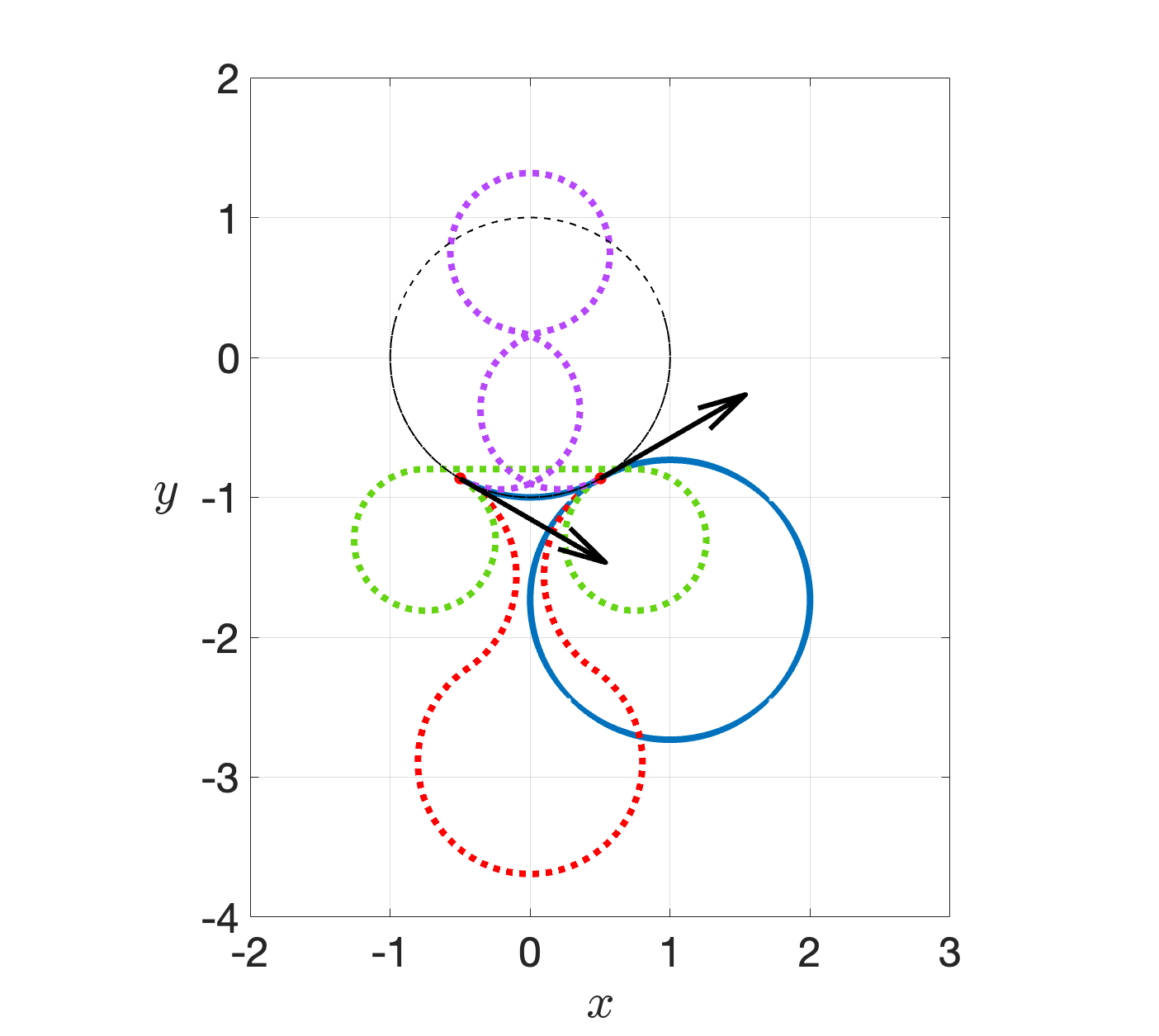
(a) : Solid curve LR (blue) with ; dotted curves, RLR (red) with , LRL (purple) with , RSR (green) with .

(b) : Solid curve RLR (red) with ; dotted curves, LR (blue) with , LRL (purple) with , RSR (green) with .

(c) : Solid curve RLR (red) with ; dotted curves, LR (blue) with , RSR (green) with , LRL (purple) with .

(d) : Solid curve RLR (red) with ; dotted curves, RSR (green) with , RLR (brown) with , LR (blue) with .
In each of the problem instances, one curve of type, two curves of type, and one curve of type have been found as solutions of Problem (Ps) by the AMPL–Knitro suite. Of these four distinct solutions in each case, the curve with the smallest was identified as the optimal curve for that case.
Similarly to Example 5.1.1, the loop in each of the curves presented in Figure 8 can be “flipped over” or “reflected about” the circle to get “symmetric” curves of type with , with the same endpoints and maximum curvatures. These reflected curves have also been encountered as computational solutions to Problem (Ps), but are not being shown in Figure 8.
We note that if then one does not encounter a solution curve (optimal or only critical) which contains a loop.
5.1.3 Example 3
Consider the problem of finding a curve of minimax curvature between the oriented points and —note that the same oriented endpoints were used in [10] for finding the shortest curve of bounded curvature, i.e., the Markov–Dubins path. For various lengths, namely for and , here we find curves minimizing the bound on the curvature. Figure 9(a)–(d) depict these curves found as a solution of Problem (Ps) by employing the AMPL–Knitro software suite.
In Figure 9(a)–(d), the optimal curves are shown as solid curves. These curves have been identified amongst all the critical solutions to Problem (Ps) (of the allowed types) that the AMPL–Knitro suite could find, as the ones with the smallest curvature, or indeed with the biggest turning radius. All other critical curves are shown as dotted curves in Figure 9(a)–(d). A summary of all these solutions in each part of Figure 9 can be given as follows, with arc lengths and curvatures correct up to 10 dp.

(a) : Solid curve LSR with .

(b) : Solid curve RLR with .

(c) : Solid curve RSR with .

(d) : Solid curve RSR with .
-
(a)
: The optimal curve has and is of type (with ), where , , . Only one other critical curve is found which has and is of type .
-
(b)
: The optimal curve has and is of type with, , . Four other critical curves are found which respectively have , , , , and are of types , , , .
-
(c)
: The optimal curve has and is of type with, , . Five other critical curves are found which respectively have , , , , and are of types , , , , .
-
(d)
: The optimal curve has and is of type with, , . Six other critical curves are found which respectively have , , , , , and are of types , , , , , .
6 Conclusion
We have presented a classification of the solutions to the problem of finding planar curves of minimax curvature between two endpoints with the endpoint tangents specified (Problem (P)). We devised a numerical procedure for finding the critical points of Problem (P), or the -elastica, of the classification types we have presented. Of these critical solutions the one with the smallest curvature is the (global) solution to Problem (P), which we refer to as a curve of minimax curvature.
A natural extension of this paper would be the study of interpolating curves which not only satisfy the endpoint constraints but also must pass through a number of specified intermediate points.
It would also be interesting to study another extension of Problem (P), from curves in to curves in . In alone, it is highly likely that one would encounter curve segments of types different from just circular and straight line segments.
A further extension from the Euclidean space to curved spaces would be of great interest where the curves of minimax curvature would be in a Riemannian manifold.
References
- [1] R. A. Adams, J. J. F. Fournier, Sobolev Spaces, Second Edition, Elsevier, 2003.
- [2] R. Andreani, E. G. Birgin, J. M. Martínez, and M. L. Schuverdt, On augmented Lagrangian methods with general lower-level constraints, SIAM J. Optim., 18(4) (2008), pp. 1286–1309.
- [3] E. G. Birgin and J. M. Martínez, Practical Augmented Lagrangian Methods for Constrained Optimization, SIAM Publications, 2014.
- [4] R. H. Byrd, J. Nocedal, R. A. Waltz, KNITRO: An integrated package for nonlinear optimization. In: G. di Pillo and M. Roma, eds., Large-Scale Nonlinear Optimization, Springer, New York, 35–59, 2006. https://doi.org/10.1007/0-387-30065-1_4
- [5] L. E. Dubins, On curves of minimal length with a constraint on average curvature and with prescribed initial and terminal positions and tangents, Amer. J. Math., 79 (1957), pp. 497–516.
- [6] R. Fourer, D. M. Gay, and B. W. Kernighan, AMPL: A Modeling Language for Mathematical Programming, Second Edition, Brooks/Cole Publishing Company / Cengage Learning, 2003.
- [7] E. Gallagher and R. Moser, The -elastica problem on a Riemannian manifold, J. Geom. Anal., 33(7) (2023), 226.
- [8] P. E. Gill, W. Murray, and M. A. Saunders, SNOPT: an SQP algorithm for large-scale constrained optimization, SIAM Rev., 47(1) (2005), 99–131.
- [9] R. Huang, A note on the -elastica in a constant sectional curvature manifold, J. Geom. Phys., 49(3–4) (2004), 343–-349.
- [10] C. Y. Kaya, Markov–Dubins path via optimal control theory, Comput. Optim. Appl., 68(3) (2017), 719–747.
- [11] C. Y. Kaya, Markov–Dubins interpolating curves, Comput. Optim. Appl., 73(2) (2019), 647–677.
- [12] C. Y. Kaya, S. K. Lucas, and S. T. Simakov, Computations for bang–bang constrained optimal control using a mathematical programming formulation, Opt. Contr. Appl. Meth., 25 (2004), 295–308.
- [13] C. Y. Kaya and J. L. Noakes, Computations and time‐optimal controls, Opt. Contr. Appl. Meth., 17 (1996), 171–185.
- [14] C. Y. Kaya and J. L. Noakes, Computational algorithm for time-optimal switching control, J. Optim. Theory App., 117 (2003), 69–92.
- [15] C. Y. Kaya and J. L. Noakes, Finding interpolating curves minimizing acceleration in the Euclidean space via optimal control theory, SIAM J. Control Optim., 51(1) (2013), 442–464.
- [16] M. G. Kreĭn and A. A. Nudel’man, The Markov Moment Problem and Extremal Problems, Translations of Mathematical Monographs, Amer. Math. Soc., 1977.
- [17] A. A. Markov, Some examples of the solution of a special kind of problem on greatest and least quantities, Soobscenija Charkovskogo Matematiceskogo Obscestva, 2-1(5,6), 250–276, 1889 (in Russian).
- [18] H. Maurer, C. Büskens, J.-H. R. Kim, and C. Y. Kaya, Optimization methods for the verification of second order sufficient conditions for bang–bang controls, Opt. Cont. Appl. Meth., 26 (2005), 129–156.
- [19] T. Miura and K. Yoshizawa, Pinned planar p-elasticae, arXiv preprint arXiv:2209.05721 (2022).
- [20] R. Moser, Structure and classification results for the -elastica problem, Amer. J. Math., 144(5) (2022), 1299–1329.
- [21] L. S. Pontryagin, V. G. Boltyanskii, R. V. Gamkrelidze, and E. F. Mishchenko, The Mathematical Theory of Optimal Processes (Russian), English translation by K. N. Trirogoff, ed. by L. W. Neustadt, Interscience Publishers, New York, 1962.
- [22] A. Wächter and L. T. Biegler, On the implementation of a primal-dual interior point filter line search algorithm for large-scale nonlinear programming, Math. Program., 106 (2006), 25–57.
- [23] K. Yosida, Functional Analysis, Fifth Edition, Springer-Verlag, 1978.