Current-driven motion of magnetic topological defects in ferromagnetic superconductors

The order parameter of a fully spin-polarized triplet superconductor provides a starting point for understanding how superconductivity and magnetism are intertwined through the emergent gauge field. In the d-vector formalism defined by $i(\mathbf{d}\cdot\boldsymbol{\sigma}\sigma^{y})_{s,s^{\prime}}\equiv\Delta_{s,s^{\prime}}$, it is given by [7, 12, 13]

$$\mathbf{d}=\frac{\sqrt{\rho}}{2}e^{i\phi}(\hat{\mathbf{u}}+i\hat{\mathbf{v}})=\sqrt{\frac{\rho}{2}}\frac{e^{i\phi}(\hat{\mathbf{u}}+i\hat{\mathbf{v}})}{\sqrt{2}}\equiv\sqrt{\frac{\rho}{2}}\hat{\mathbf{d}}\,,$$

(1)

where $\rho=2\mathbf{d}^{*}\cdot\mathbf{d}$ is the number density of the Cooper pairs, $\hat{\mathbf{u}}$ and $\hat{\mathbf{v}}$ are perpendicular unit vectors, and $\hat{\mathbf{d}}^{*}\cdot\hat{\mathbf{d}}=1$; the simplest example would be $\hat{\mathbf{u}}=\hat{\mathbf{x}},\hat{\mathbf{v}}=\hat{\mathbf{y}}$ which gives $\Delta_{s,s^{\prime}}=0$ except for $\Delta_{\uparrow\uparrow}$ (see Appendix A for the details). There is an ambiguity here in defining $\phi$ as the above order parameter remains invariant under the following simultaneous change of $\phi$ and $\hat{\mathbf{u}}$ and $\hat{\mathbf{v}}$:

$$e^{i\phi}(\hat{\mathbf{u}}+i\hat{\mathbf{v}})=e^{i(\phi+\delta\phi)}\left[e^{-i\delta\phi}(\hat{\mathbf{u}}+i\hat{\mathbf{v}})\right]\equiv e^{i(\phi+\delta\phi)}(\hat{\mathbf{u}}^{\prime}+i\hat{\mathbf{v}}^{\prime})\,,$$

(2)

where $\hat{\mathbf{u}}^{\prime},\hat{\mathbf{v}}^{\prime}$ are obtained by rotating $\hat{\mathbf{u}},\hat{\mathbf{v}}$ by $+\delta\phi$ around $\hat{\mathbf{u}}\times\hat{\mathbf{v}}$. As the spin density in units of $\hbar$ can be written as

$$\mathbf{s}=2i\mathbf{d}\times\mathbf{d}^{*}=\rho\hat{\mathbf{u}}\times\hat{\mathbf{v}}\equiv\rho\hat{\mathbf{s}}\,,$$

(3)

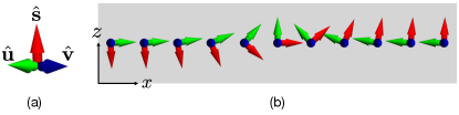
Eq. (2) denotes the ${\rm U}(1)_{\phi+s}$ order parameter redundancy [7, 12], i.e. the invariance of the order parameter when the angle of the spin rotation around $\hat{\mathbf{s}}$ equals the change in $\phi$. Such redundancy implies the existence of an effective gauge field arising from the spin degrees of freedom. See Fig. 1(a) for the illustration of the three mutually orthogonal unit vectors $\hat{\mathbf{s}},\hat{\mathbf{u}}$, and $\hat{\mathbf{v}}$, which are depicted by red, green, and blue arrows, respectively.

For deriving the vector potential and magnetostatics of this effective gauge field, the above order parameter suffices. From the spin rotation angle around $\hat{\bf s}$ defined as $\alpha$, the effective vector gauge can be written as [14]

$$a_{i}\equiv\frac{\hbar}{q}\partial_{i}\alpha=\frac{\hbar}{q}\hat{\mathbf{s}}\cdot(\hat{\mathbf{u}}\times\partial_{i}\hat{\mathbf{u}})\,;$$

(4)

hence the emergent gauge is a direct consequence of the ${\rm U}(1)_{\phi+s}$ order parameter redundancy of Eq. (2). Indeed, the emergent gauge field of spatial curvature in the chiral superconductor has been attributed to the analogous order parameter redundancy there [22, 23, 24, 25]. Here, while we have kept the charge, $q$, generic, $q=-2e<0$ holds in superconductors. From this emergent vector potential, it is straightforward to obtain the emergent magnetic field,

$$b_{i}=\epsilon_{ijk}\partial_{j}a_{k}=-\frac{\hbar\epsilon_{ijk}}{2q}\hat{\mathbf{s}}\cdot(\partial_{j}\hat{\mathbf{s}}\times\partial_{k}\hat{\mathbf{s}})\,;$$

(5)

note that this is in the same form as the well-known Mermin-Ho relation between the orbital angular momentum texture and superfluid velocity in the 3He-A superfluid [26, 27]. Yet this discussion does not include any dynamics, for which we shall adopt a two-step approach of first formulating the simplest free energy for the order parameter [Eq. (2)] and then use its Lagrangian to obtain the equations of motion.

Given that we seek results relevant to wide-ranging superconductors whose common attributes may not extend beyond the spin-polarized Cooper pairing [1, 2, 3, 4, 5, 6] we will consider for our free energy the simplest minimal model that includes the spin anisotropy and the Zeeman coupling:

$$F[\mathbf{d}]=\int dV\mathcal{F}^{\prime}_{0}[\mathbf{d}]+\int dV\frac{U}{2}\left(2|\mathbf{d}|^{2}-\rho_{0}\right)^{2}\,,$$

(6)

where

$$\mathcal{F}^{\prime}_{0}\!=\!\frac{A^{\prime}_{d}}{2}|(\boldsymbol{\nabla}-i\frac{q}{\hbar}\mathbf{A})\mathbf{d}|^{2}+\rho\!\left[\frac{A^{\prime}_{s}}{2}|\boldsymbol{\nabla}\hat{\mathbf{s}}|^{2}\!-\!\frac{D}{2}(\hat{\mathbf{s}}\!\cdot\!\hat{\mathbf{z}})^{2}\!-\!Hs_{z}\!+\!qV\right]\,,$$

where $A^{\prime}_{s}$ represents the excess spin stiffness; note that, in contrast to previous analysis [12], our treatment will encompass both the easy-axis anisotropy $D>0$ and the easy-plane anisotropy $D<0$. As we will focus on the cases where the fluctuation of the condensate density $\rho\equiv 2|\mathbf{d}|^{2}$ is strongly suppressed, it is convenient to separately group together terms dependent on $\rho$ fluctuations [12, 13]

$$F=\int dV\rho\mathcal{F}_{0}+\int dV\left[\frac{A^{\prime}_{d}}{16\rho}(\boldsymbol{\nabla}\rho)^{2}+\frac{U}{2}(\rho-\rho_{0})^{2}\right]\,,$$

where

$$\mathcal{F}_{0}=\frac{A^{\prime}_{d}}{2}|(\boldsymbol{\nabla}-i\frac{q}{\hbar}\mathbf{A})\hat{\mathbf{d}}|^{2}+\frac{A^{\prime}_{s}}{2}|\boldsymbol{\nabla}\hat{\mathbf{s}}|^{2}-\frac{D}{2}(\hat{\mathbf{s}}\cdot\hat{\mathbf{z}})^{2}-Hs_{z}+qV$$

is the free energy density per unit density. The gauge transformation is implemented as

$$\mathbf{A}\mapsto\mathbf{A}+\boldsymbol{\nabla}\Lambda\,,\quad\mathbf{d}\mapsto e^{iq\Lambda/\hbar}\mathbf{d}\,.$$

The free energy can be recast into the following form:

$$F=\int dV\rho\left\{\frac{A_{c}}{2}\left[\partial_{i}\phi-\frac{q}{\hbar}A_{i}-\hat{\mathbf{s}}\cdot(\hat{\mathbf{u}}\times\partial_{i}\hat{\mathbf{u}})\right]^{2}+\frac{A_{s}}{2}(\partial_{i}\hat{\mathbf{s}})^{2}-\frac{D}{2}(\hat{\mathbf{s}}\cdot\hat{\mathbf{z}})^{2}-Hs_{z}+qV\right\}+\int dV\left[\frac{A_{c}}{8\rho}(\boldsymbol{\nabla}\rho)^{2}+\frac{U}{2}(\rho-\rho_{0})^{2}\right]\,,$$

(7)

where $A_{c}=A^{\prime}_{d}$ and $A_{s}=A^{\prime}_{s}+A^{\prime}_{d}/2$. Here, $A_{c}$ and $A_{s}$ represent the charge stiffness and the spin stiffness, respectively. The similar expression without the second and the third terms can be found in Eq. (2.3) and Eq. (2.5) of Ref. [28].

Accordingly, the charge supercurrent density is modified to

$$J_{i}=-\frac{\delta F}{\delta A_{i}}=\frac{q}{\hbar}\rho A_{c}(\partial_{i}\phi-\frac{q}{\hbar}A_{i}-\frac{q}{\hbar}a_{i})\,,$$

(8)

with the velocity field is given by

$$v_{i}=\frac{J_{i}}{q\rho}=\frac{A_{c}}{\hbar}(\partial_{i}\phi-\frac{q}{\hbar}A_{i}-\frac{q}{\hbar}a_{i})\,.$$

(9)

It satisfies the following equation (by assuming a nonsingular $\theta$):

$$\boldsymbol{\nabla}\times\mathbf{v}=-\frac{qA_{c}}{\hbar^{2}}(\mathbf{B}+\mathbf{b})\,.$$

(10)

The free energy formalism provides a convenient springboard for extending our analysis to dynamics as well. In particular, such analysis helps us understand how emergent electric field would arise, in analogy with the standard electrodynamics. This is accomplished by considering the Langrangian for this minimal model.

For the dynamics analysis, we now obtain the classical equation of motion for both the charge and the spin component of the order parameter through considering the Lagrangian of the spin-polarized superconductor. This can be written as

	$\displaystyle L$	$\displaystyle=$	$\displaystyle\int dV2i\hbar\mathbf{d}^{*}\cdot\partial_{t}\mathbf{d}-F\,$		(11)
		$\displaystyle=$	$\displaystyle-\int dV\hbar\rho[\partial_{t}\phi-\hat{\mathbf{s}}\cdot(\hat{\mathbf{u}}\times\partial_{t}\hat{\mathbf{u}})]-F\,.$

The first term of the above Lagrangian arises from $2i\hbar{\bf d}^{*}$ being the conjugate variable to ${\bf d}$; the detailed derivation of its relation to $\rho,\phi,\hat{\mathbf{s}}$ can be found in Appendix B. The low-energy dynamics of the order parameter can be described by the three Euler-Lagrange equations for $\phi,\rho$, and $\hat{\mathbf{s}}$.

The equations for $\rho$ and $\phi$ are basically analogous to those of the conventional superconductors. The equation of motion for the density $\rho$,

	$\displaystyle\dot{\rho}$	$\displaystyle=$	$\displaystyle-\frac{1}{\hbar}\partial_{i}\left\{\rho A_{c}\left[\partial_{i}\phi-\frac{q}{\hbar}A_{i}-\hat{\mathbf{s}}\cdot(\hat{\mathbf{u}}\times\partial_{i}\hat{\mathbf{u}})\right]\right\}=-\frac{1}{q}\partial_{i}J_{i}\,,$		(12)
		$\displaystyle=$	$\displaystyle-\boldsymbol{\nabla}\cdot(\rho\mathbf{v})\,$

is obtained from $\delta L/\delta\phi=0$ and is none other than the continuity equation for the Cooper pair density. Similarly, the equation of motion for the phase $\phi$

$$-\hbar[\partial_{t}\phi-\hat{\mathbf{s}}\cdot(\hat{\mathbf{u}}\times\partial_{t}\hat{\mathbf{u}})]=\mathcal{F}_{0}+U(\rho-\rho_{0})-\frac{A_{c}}{4\rho}\nabla^{2}\rho\,$$

(13)

obtained from $\delta L/\delta\rho=0$ (where only terms constant or linear in $\rho$ are retained) comes out to be the Josephson relation. We, however, want to obtain a hydrodynamic equation of motion for Cooper pairs, for which purpose we take the spatial derivative of the Josephson relation:

$$-\hbar\left[\partial_{t}\partial_{i}\phi-\frac{q}{\hbar}(E_{i}+e_{i})-\frac{q}{\hbar}\partial_{t}(A_{i}+a_{i})\right]=\frac{\hbar^{2}}{A_{c}}\mathbf{v}\cdot\partial_{i}\mathbf{v}+\partial_{i}\left[\rho^{\prime}_{e}+U(\rho-\rho_{0})-\frac{A_{c}}{4\rho}\nabla^{2}\rho\right]\,,$$

where

$$e_{i}=-\frac{\hbar}{q}\hat{\mathbf{s}}\cdot(\partial_{i}\hat{\mathbf{s}}\times\partial_{t}\hat{\mathbf{s}})\,$$

(14)

is the emergent electric field and

$$\rho^{\prime}_{e}=A_{s}\frac{(\partial_{i}\hat{\mathbf{s}})^{2}}{2}-D\frac{s_{z}^{2}}{2}-Hs_{z}$$

(15)

is the magnetic energy density (per unit density). By using

$$\mathbf{v}\cdot\partial_{i}\mathbf{v}=\frac{1}{2}\partial_{i}(\mathbf{v}^{2})=(\mathbf{v}\cdot\boldsymbol{\nabla})v_{i}+\epsilon_{ijk}v_{j}(\boldsymbol{\nabla}\times\mathbf{v})_{k}=(\mathbf{v}\cdot\boldsymbol{\nabla})v_{i}-\frac{qA_{c}}{\hbar^{2}}\epsilon_{ijk}v_{j}(B_{k}+b_{k})\,$$

and defining the material derivative $D_{t}\equiv\partial_{t}+\mathbf{v}\cdot\boldsymbol{\nabla}$ and the effective mass of a Cooper pair, $m\equiv\hbar^{2}/A_{c}$, we obtain

$$mD_{t}\mathbf{v}=q(\mathbf{E}+\mathbf{e})+q\mathbf{v}\times(\mathbf{B}+\mathbf{b})-\partial_{i}\left[\rho^{\prime}_{e}+U(\rho-\rho_{0})-\frac{A_{c}}{4\rho}\nabla^{2}\rho\right]\,.$$

(16)

The novelty in the ferromagnetic superconductor is the equation of motion for the spin direction $\hat{\mathbf{s}}$ that is derived from $\delta L/\delta\hat{\mathbf{s}}=0$ (see Appendix C for details):

$$\hbar\rho\partial_{t}\hat{\mathbf{s}}=-\frac{\hbar J_{i}}{q}\partial_{i}\hat{\mathbf{s}}+\partial_{i}[\rho A_{s}(\hat{\mathbf{s}}\times\partial_{i}\hat{\mathbf{s}})]+\rho D(\hat{\mathbf{s}}\cdot\hat{\mathbf{z}})\hat{\mathbf{s}}\times\hat{\mathbf{z}}+\rho H\hat{\mathbf{s}}\times\hat{\mathbf{z}}\,,$$

(17)

which is identical to the Landau-Lifshitz equation [29] augmented by the adiabatic spin-transfer torque [30, 31, 9]. This can be also written as

$$\hbar\rho D_{t}\hat{\mathbf{s}}=\partial_{i}[\rho A_{s}(\hat{\mathbf{s}}\times\partial_{i}\hat{\mathbf{s}})]+\rho D(\hat{\mathbf{s}}\cdot\hat{\mathbf{z}})\hat{\mathbf{s}}\times\hat{\mathbf{z}}+\rho H\hat{\mathbf{s}}\times\hat{\mathbf{z}}\,.$$

By using $\dot{\rho}=-\partial_{i}J_{i}/q$, we can obtain the spin continuity equation:

$\displaystyle\partial_{t}(\hbar\rho\hat{\mathbf{s}})=-\partial_{i}\mathbf{J}^{s}_{i}+\rho D(\hat{\mathbf{s}}\cdot\hat{\mathbf{z}})\hat{\mathbf{s}}\times\hat{\mathbf{z}}+\rho H\hat{\mathbf{s}}\times\hat{\mathbf{z}}\,,$

(18)

where

$$\mathbf{J}^{s}_{i}=\frac{\hbar J_{i}}{q}\hat{\mathbf{s}}-\rho A_{s}(\hat{\mathbf{s}}\times\partial_{i}\hat{\mathbf{s}})\,,$$

is the spin current density. The first term and the second term on the right-hand side are longitudinal spin currents proportional to the charge current and the transverse spin current that is carried by a spin texture, respectively.

A complete set of equations describing the hydrodynamics of a ferromagnetic superconductor in the absence of external fields ($\mathbf{E}=0$ and $\mathbf{B}=0$) can now be given; the analogous equations have been written down for a spinor BEC [32]. It is convenient to measure energy in the unit of the anisotropy energy absolute value $|D|$ and length in the unit derived from the combination of $|D|$ with the spin stiffness $A_{s}$, i.e.

$$l=\sqrt{\frac{A_{s}}{|D|}}\,,\quad\epsilon=|D|\,.$$

Also, we will use $\tilde{\rho}\equiv\rho/\rho_{0},U\rho/D\equiv\eta$. This gives us the dimensionless equations

	$\displaystyle-D_{t}\tilde{\rho}$	$\displaystyle=$	$\displaystyle\tilde{\rho}(\boldsymbol{\nabla}\cdot\mathbf{v})\,,$
	$\displaystyle\tilde{m}(\boldsymbol{\nabla}\times\mathbf{v})$	$\displaystyle=$	$\displaystyle-\mathbf{b}\,,$
	$\displaystyle\tilde{m}D_{t}\mathbf{v}$	$\displaystyle=$	$\displaystyle\mathbf{e}+\mathbf{v}\times\mathbf{b}$
			$\displaystyle-\partial_{i}[\rho_{e}\!+\!\eta(\tilde{\rho}-1)-\nabla^{2}\tilde{\rho}/4]\,,$
	$\displaystyle\tilde{\rho}D_{t}\hat{\mathbf{s}}$	$\displaystyle=$	$\displaystyle\partial_{i}[\tilde{\rho}(\hat{\mathbf{s}}\times\partial_{i}\hat{\mathbf{s}})]+\tilde{\rho}\nu(\hat{\mathbf{s}}\cdot\hat{\mathbf{z}})\hat{\mathbf{s}}\times\hat{\mathbf{z}}+\tilde{\rho}h\hat{\mathbf{s}}\times\hat{\mathbf{z}}\,,$

where $\nu\equiv{\rm sgn}(D)$, $\tilde{m}\equiv A_{s}/A_{c}$ the dimensionless mass which is on the order of unity, $h\equiv H/D$ the dimensionless external field, and

$$\rho_{e}=\frac{1}{2}(\partial_{i}\hat{\mathbf{s}})^{2}-\nu\frac{1}{2}(\hat{\mathbf{s}}\cdot\hat{\mathbf{z}})^{2}-hs_{z}$$

the dimensionless magnetic energy density; for zero excess spin stiffness $\tilde{m}=1/2$. The emergent electromagnetic fields are now re-defined as

$$e_{i}=-\hat{\mathbf{s}}\cdot(\partial_{i}\hat{\mathbf{s}}\times\partial_{t}\hat{\mathbf{s}})\,,\quad b_{i}=-\frac{\epsilon_{ijk}}{2}\hat{\mathbf{s}}\cdot(\partial_{j}\hat{\mathbf{s}}\times\partial_{k}\hat{\mathbf{s}})\,,$$

where the charge $q$ is absorbed into the fields.

Due to the inevitable nonconservation of spin angular momentum in solids, it is reasonable to expect the damping of spin dynamics and the associated energy dissipation, which are not included in the hydrodynamics equations [Eq. (LABEL:EQ:hydro)], to play an important role in spin dynamics of the ferromagnetic superconductors as in any other solid-state systems. The spin sinks can be quasiparticles, phonons, and any other excitations that can possess angular momentum [33, 34, 35, 36]. The spin dissipation can be treated phenomenologically with the addition of the Gilbert damping term $\alpha\tilde{\rho}\hat{\mathbf{s}}\times\partial_{t}\hat{\mathbf{s}}$ [8] to the spin equation of motion in Eq. (LABEL:EQ:hydro),

$$\tilde{\rho}D_{t}\hat{\mathbf{s}}+\alpha\tilde{\rho}\hat{\mathbf{s}}\times\partial_{t}\hat{\mathbf{s}}=\partial_{i}[\tilde{\rho}(\hat{\mathbf{s}}\times\partial_{i}\hat{\mathbf{s}})]+\tilde{\rho}\nu(\hat{\mathbf{s}}\cdot\hat{\mathbf{z}})\hat{\mathbf{s}}\times\hat{\mathbf{z}}+\tilde{\rho}h\hat{\mathbf{s}}\times\hat{\mathbf{z}}\,.$$

(20)

In the incompressible limit $\eta\rightarrow\infty$ where $\tilde{\rho}$ is uniform and constant, this gives us the energy continuity equation,

$$\partial_{t}\rho_{e}+\boldsymbol{\nabla}\cdot\mathbf{j}_{e}=-\mathbf{v}\cdot\mathbf{e}-\alpha(\partial_{t}\hat{\mathbf{s}})^{2}\,,$$

(21)

where

$$\mathbf{j}_{e}=-\partial_{t}\hat{\mathbf{s}}\cdot\boldsymbol{\nabla}\hat{\mathbf{s}}$$

(22)

is the magnetic energy flux density (per unit density). This continuity equation, which has been previously noted in literature [37, 38], can be derived by taking the product of both sides of Eq. (20) with $\hat{\mathbf{s}}\times\partial_{t}\hat{\mathbf{s}}$. One can note that the first term on the right-hand side of Eq. (21) ($-\mathbf{v}\cdot\mathbf{e}$) is the power dissipated (supplied) by the superflow $\mathbf{v}$ flowing parallel (antiparallel) to the direction of the emergent electric field $\mathbf{e}$, while the second term ($-\alpha(\partial_{t}\hat{\mathbf{s}})^{2}$) is the energy dissipation through the Gilbert damping.

Equation (21) implies that, in the incompressible limit, the energy dissipated by the Gilbert damping is equal to the work done by the emergent electric field when spin texture is transported without any distortion. This is because the total magnetic energy should be unchanged in this process and hence the left-hand side of Eq. (21) integrated over the whole system should be zero.

The solution for a domain-wall motion in the background of the constant and uniform background superflow can be straightforwardly constructed from the static domain wall solution in absence of any background superflow for the incompressible limit $\eta\to\infty$. For this case, the absence of the emergent magnetic field allows us to consider only the spin equation of motion [40]

$$(\partial_{t}+\mathbf{v}\cdot\boldsymbol{\nabla}+\alpha\hat{\mathbf{s}}\times\partial_{t})\hat{\mathbf{s}}=\partial_{i}[(\hat{\mathbf{s}}\times\partial_{i}\hat{\mathbf{s}})]+(\hat{\mathbf{s}}\cdot\hat{\mathbf{z}})\hat{\mathbf{s}}\times\hat{\mathbf{z}}\,;$$

(23)

from the hydrodynamic equations Eq. (LABEL:EQ:hydro); others are either irrelevant due to ${\bf b}=0$ or merely provides the constraint $\tilde{\rho}=1$ in the incompressible limit. Given the intrinsically quasi-one-dimensional nature of the domain wall, we can set the boundary condition

$$\hat{\mathbf{s}}(x\rightarrow\pm\infty)=\pm\hat{\mathbf{z}}\,,$$

for any domain-wall configuration. For the static domain wall at $x=0$ in absence of background superflow, the solution is given by the following Walker ansatz [41]:

$$\hat{\mathbf{s}}_{0}=(\hat{\mathbf{x}}\cos\varphi_{0}+\hat{\mathbf{y}}\sin\varphi_{0})\mathrm{sech}x+Q\hat{\mathbf{z}}\tanh x,$$

(24)

where $Q=\pm 1$ represents the domain wall type, satisfies the static domain-wall equation

$$0=\partial_{x}[(\hat{\mathbf{s}}_{0}\times\partial_{x}\hat{\mathbf{s}}_{0})]+(\hat{\mathbf{s}}_{0}\cdot\hat{\mathbf{z}})\hat{\mathbf{s}}_{0}\times\hat{\mathbf{z}}\,,$$

(25)

derived from Eq. (23), for an arbitrary domain-wall angle $\varphi_{0}$; it is important to note here that Eq. (25) is sufficient as Eq. (24) gives us ${\bf v}=0$ and ${\bf b}=0$ everywhere.

From Eq. (25), it can be shown that the general solution can be obtained by applying to the static solution both giving boost in the spatial direction and precession around the easy-axis:

$$\hat{\mathbf{s}}=(\hat{\mathbf{x}}\cos\Omega t+\hat{\mathbf{y}}\sin\Omega t)\mathrm{sech}(x-Vt)+Q\hat{\mathbf{z}}\tanh(x-Vt)\,.$$

(26)

In deriving the domain-wall velocity $\hat{\mathbf{x}}V$ and the precession rate $\Omega$, it is convenient to note that Eq. (26) also satisfies Eq. (25) as the latter equation involves no time derivatives. Also, as Eq. (26) is obtained from boost and precession,

$$\partial_{t}\hat{\mathbf{s}}=(-V\partial_{x}+\hat{\mathbf{z}}\Omega\times)\hat{\mathbf{s}}\,.$$

The velocity $V$ and the precession rate $\Omega$ therefore can be obtained from

$$[v\partial_{x}+(1+\alpha\hat{\mathbf{s}}\times)(-V\partial_{x}+\hat{\mathbf{z}}\Omega\times)]\hat{\mathbf{s}}=0\,,$$

(27)

where we set the background superflow to be perpendicular to the domain wall without any loss of generality, $\mathbf{v}=v\hat{\mathbf{x}}$. By taking the scalar product of the above equation with $\hat{\mathbf{z}}$ and $\hat{\mathbf{z}}\times\hat{\mathbf{s}}$ we obtain

$$v-V=Q\alpha\Omega\,,\quad\Omega=-Q\alpha V$$

respectively, giving us

$$V=\frac{1}{1+\alpha^{2}}v\,,\quad\Omega=-\frac{Q\alpha}{1+\alpha^{2}}v\,;$$

(28)

Note that in absence of the Gilbert damping, $\alpha=0$, there would have been no precession and the domain wall would have remained static with respect to the background superflow. See Fig. 2 for the illustration of the domain-wall dynamics with precession.

From the above solution, it is straightforward to confirm that all work done by the emergent electric field is dissipated through the Gilbert damping. The work done by the emergent electric field is

$$-\mathbf{v}\cdot\mathbf{e}=v_{j}\hat{\mathbf{s}}\cdot(\partial_{j}\hat{\mathbf{s}}\times\partial_{t}\hat{\mathbf{s}})=Qv\Omega[1-(\hat{\mathbf{s}}\cdot\hat{\mathbf{z}})^{2}]\,,$$

(29)

which gives the total energy input of

$$W=\int dx(-\mathbf{v}\cdot\mathbf{e})=2Qv\Omega\,.$$

(30)

The energy dissipation rate per unit density is given by

$$\alpha(\partial_{t}\hat{\mathbf{s}})^{2}=\alpha(V^{2}+\Omega^{2})[1-(\hat{\mathbf{s}}\cdot\hat{\mathbf{z}})^{2}]\,.$$

(31)

This energy dissipation through the spin dynamics and the work rate done by the emergent electric field on the superflow are the same since

$$Qv\Omega=\frac{\alpha}{1+\alpha^{2}}v^{2}$$

(32)

and

$$\alpha(V^{2}+\Omega^{2})=\frac{\alpha}{1+\alpha^{2}}v^{2}\,.$$

(33)

Due to the U(1)_ϕ+s order parameter redundancy, the energy dissipation from the damping-induced precession in the domain-wall motion can be regarded as an equivalent of $4\pi$ phase slips. As shown in Fig. 2, $\hat{\mathbf{u}}$ and $\hat{\mathbf{v}}$ rotate around $\hat{\mathbf{s}}$ by $\pm 2\pi$ by adiabatically following the dynamics of the local spin direction $\hat{\mathbf{s}}$ in one cycle of precession. To see this, note that if we adopt the condition $\hat{\mathbf{v}}\cdot\hat{\mathbf{z}}=0$ in defining $\hat{\mathbf{v}}$, Eq. (26) will give us $\hat{\mathbf{v}}=-\hat{\mathbf{x}}\sin\Omega t+\hat{\mathbf{y}}\cos\Omega t$. But given the U(1)_ϕ+s redundancy, this is equivalent to the $\pm 2\pi$ phase twist on the left and the right end, respectively.

The voltage arising from this precession can be understood either as arising from the emergent electric field, or equivalently, arising from the constant rate of $4\pi$ phase slips. When $\varphi$ increases at the rate $\dot{\varphi}=\Omega$, the emergent scalar potential at the two ends of the wire, $x=\pm\infty$, is given by

$$\tilde{V}_{e}=-\hat{\mathbf{s}}\cdot(\hat{\mathbf{u}}\times\partial_{t}\hat{\mathbf{u}})=\begin{cases}-Q\Omega&\text{ at }x=-\infty\,,\\ Q\Omega&\text{ at }x=\infty\,,\end{cases}$$

(34)

which is exactly the Josephson voltage for the $4Q\pi$ phase slip occurring at the rate of $\Omega/2\pi$. Then, to maintain the finite superflow, there must be work given by

$$W=v[\tilde{V}_{e}(x=\infty)-\tilde{V}_{e}(x=-\infty)]=2Qv\Omega\,,$$

(35)

by external reservoirs on the system, matching the work [Eq. (30)]. Figure 2(a) shows the time evolution of the triad {$\hat{\mathbf{s}},\hat{\mathbf{u}},\hat{\mathbf{v}}$} associated with the domain-wall that both moves and precesses. Note that $\hat{\mathbf{u}}$ (green arrow) at the left end ($x\rightarrow-\infty$) and the right end ($x\rightarrow\infty$) rotates clockwise and counterclockwise, respectively, about $\hat{\mathbf{s}}$ (red arrow), engendering the nonsingular phase slips across the $x$ direction. In a nutshell, the domain-wall angular dynamics produces the nonsingular $4\pi$ phase slips that give rise to a finite voltage difference between the two ends of the superconducting wire, which constitutes our first main result.

There is a topological reason why one precession of a magnetic domain wall induces a $4\pi$ phase slip, which can be derived from the Poincaré-Hopf theorem or Poincaré-Brower theorem [39]. For concrete discussion on this, we will consider in the following the case with $Q=1$ as shown in Fig. 2(b) and (c). At a given time, the instantaneous configuration of $\hat{\mathbf{s}}$ and $\hat{\mathbf{u}}$ can be mapped onto a line connecting the north pole [$\hat{\mathbf{s}}(x\rightarrow\infty)]$ and the south pole [$\hat{\mathbf{s}}(x\rightarrow-\infty)$] on the unit sphere by identifying $\hat{\mathbf{s}}$ with the surface normal as shown in Fig. 2(b). When we consider the collection of the configuration of {$\hat{\mathbf{s}},\hat{\mathbf{u}}$} onto the unit sphere during one complete precession of the domain wall, i.e., $\varphi_{0}\rightarrow\varphi_{0}+2\pi$, $\hat{\mathbf{u}}$ can be regarded as a unit tangent vector field on the sphere since it is perpendicular to $\hat{\mathbf{s}}$, i.e., the surface normal as shown in Fig. 2(c). Here, note that $\hat{\mathbf{u}}$ is not uniquely determined at the north pole and the south pole, which is consistent with the well-known topological property of the sphere that the unit tangent vector field cannot be defined without a singularity on it. Instead of being uniquely determined, $\hat{\mathbf{u}}$ rotates by $2\pi$ around the north pole and rotates by $-2\pi$ around the south pole as the domain wall completes one cycle of precession, which gives rise to a $4\pi$ phase slip across the wire as discussed above [Eq. (34)]. This can be understood by applying the Poincaré-Hopf theorem to the unit tangent vector field $\hat{\mathbf{u}}$ on the sphere. The Euler number of the unit sphere is 2, meaning that the sum of the indices of the isolated singularities of the unit tangent vector field on the sphere must be 2. In our case, the indices of the north pole and the south pole associated with $\hat{\mathbf{u}}$ are both 1, adding up to 2, agreeing with the Euler number of the unit sphere.

Analogous to the case of the domain wall in the previous section, a straightforward construction of the meron motion solution here in the background of the constant and uniform background superflow is possible from the static meron solution in absence of any background superflow for the incompressible limit, $\eta\rightarrow\infty$ [46, 32]. The static solution can be obtained from the following two equations;

	$\displaystyle\tilde{m}(\boldsymbol{\nabla}\times\mathbf{v})$	$\displaystyle=$	$\displaystyle-\mathbf{b}\,,$
	$\displaystyle(\mathbf{v}\cdot\boldsymbol{\nabla})\hat{\mathbf{s}}$	$\displaystyle=$	$\displaystyle\partial_{i}[(\hat{\mathbf{s}}\times\partial_{i}\hat{\mathbf{s}})]-(\hat{\mathbf{s}}\cdot\hat{\mathbf{z}})\hat{\mathbf{s}}\times\hat{\mathbf{z}}\,.$		(36)

It is important to note here that while we are dealing with a static configuration we still have ${\bf v}\neq 0$ due to the intrinsic emergent magnetic flux of the meron. In addition, this solution would possess the axial symmetry, i.e.

$$\hat{\mathbf{s}}_{0}=(\sin\theta\cos\varphi,\sin\theta\sin\varphi,\cos\theta)\,,$$

(37)

with $\theta=\theta(r)$ and $\varphi=n\chi+\Phi$ where $(r,\chi)$ are polar coordinates for the two-dimensional system, and follow the universal boundary conditions for merons are given by

$$\theta(r=0)=(1-p)\frac{\pi}{2}\,,\quad\theta(r\to\infty)=\frac{\pi}{2}\,;$$

$p=\pm 1$ here is the polarity, which is the $z$-component of the local spin direction $\hat{\mathbf{s}}$ at the meron center, and $n\in\mathbb{Z}$ the vorticity, which counts how many times $\hat{\mathbf{s}}$ winds in the easy plane along the closed trajectory encircling the meron center. For our purpose, obtaining the differential equation for $\theta(r)$ is sufficient for showing Eq. (37) to be the solution of Eq. (36). We start by noting that the emergent magnetic field is aligned entirely along the $z$-axis and

$$b_{z}=-\hat{\mathbf{s}}_{0}\cdot(\partial_{x}\hat{\mathbf{s}}_{0}\times\partial_{y}\hat{\mathbf{s}}_{0})=-\frac{n\sin\theta}{r}\frac{d\theta}{dr}\,$$

(38)

is function only for $\theta$, which gives us the well-known result

$$\int dxdyb_{z}=\int rd\chi dr\left(-\frac{n\sin\theta}{r}\frac{d\theta}{dr}\right)=-2\pi pn\,$$

(39)

for the total emergent magnetic flux. With this emergent magnetic field, the first equation of Eq. (36) requires the circulating velocity $\mathbf{v}=\hat{\boldsymbol{\varphi}}v(r)$ around the meron with

$$\frac{1}{r}\frac{d(rv)}{dr}=\frac{n\sin\theta}{\tilde{m}r}\frac{d\theta}{dr}\,.$$

Inserting this relation into the second equation of Eq. (36) gives us

$$\sin\theta(1-\cos\theta)\frac{1}{\tilde{m}r^{2}}=\frac{1}{r}\frac{d}{dr}\left(r\frac{d\theta}{dr}\right)+\cos\theta\sin\theta\left(1-\frac{1}{r^{2}}\right)\,,$$

from which $\theta(r)$ can be obtained numerically.

To find explicit expressions for $\hat{\mathbf{u}}$ and $\hat{\mathbf{v}}$, note that the following three unit vectors form an orthonormal triad:

	$\displaystyle\hat{\mathbf{s}}_{0}=\hat{\mathbf{e}}_{r}$	$\displaystyle\equiv$	$\displaystyle(\sin\theta\cos\varphi,\sin\theta\sin\varphi,\cos\theta)\,,$
	$\displaystyle\hat{\mathbf{e}}_{\theta}$	$\displaystyle\equiv$	$\displaystyle(\cos\theta\cos\varphi,\cos\theta\sin\varphi,-\sin\theta)\,,$
	$\displaystyle\hat{\mathbf{e}}_{\varphi}$	$\displaystyle\equiv$	$\displaystyle(-\sin\varphi,\cos\varphi,0)\,,$

which gives us

	$\displaystyle\hat{\mathbf{u}}_{0}(r,\chi)=\cos\varphi(\chi)\,\hat{\mathbf{e}}_{\theta}(r,\chi)-\sin\varphi(\chi)\,\hat{\mathbf{e}}_{\varphi}(r,\chi)\,,$		(40)
	$\displaystyle\hat{\mathbf{v}}_{0}(r,\chi)=\sin\varphi(\chi)\,\hat{\mathbf{e}}_{\theta}(r,\chi)+\cos\varphi(\chi)\,\hat{\mathbf{e}}_{\varphi}(r,\chi)\,.$		(41)

The local configuration of the triad $(\hat{\mathbf{s}}_{0},\hat{\mathbf{u}}_{0},\hat{\mathbf{v}}_{0})$ for a meron with $p=1$ and $n=1$ is shown in Fig. 3. Note that it is nonsingular, differing from a conventional vortex of a $s$-wave superconductor [10]. An analogous nonsingular topological defects that give rise to $4\pi$ nonsingular phase slips has been discussed by Anderson and Toulouse [47] and has been termed the skyrmion solution in the more recent literature [28, 32]. By contrast, our solution {$\hat{\mathbf{s}}_{0},\hat{\mathbf{u}}_{0},\hat{\mathbf{v}}_{0}$} [Eqs. (37,40,41)] represents an explicit solution for the nonsingular topological defect in the easy-plane case that gives rise to $2\pi$ nonsingular phase slip, as can be seen from Eqs (36) and (39): it harbors the emergent magnetic flux $-2\pi pn$ and thus its motion gives rise to the emergent electric field, i.e., phase slips perpendicular to its motion.

The non-trivial emergent gauge field $a_{i}$, and thus the quantized non-zero emergent magnetic flux, of our nonsingular topological defect can be understood from the rotation of $\hat{\mathbf{u}}$ around $\hat{\mathbf{s}}$ as stated in Eq. (4). There exists a topological constraint dictating that a meron texture of $\hat{\mathbf{s}}$ should trap a quantized non-zero emergent magnetic flux, which can be understood by invoking the Poincaré-Hopf theorem [39, 27] as follows. For the given meron configuration with $p=1$, let us consider the mapping of two unit vectors $\hat{\mathbf{s}}$ and $\hat{\mathbf{u}}$ onto the northern hemisphere such that $\hat{\mathbf{s}}$ is identified with the surface normal. Then, $\hat{\mathbf{u}}$ becomes a unit tangent vector field on the hemisphere since it is perpendicular to $\hat{\mathbf{s}}$, i.e., the surface normal as shown in Fig. 3(c). The Euler number of the hemisphere is 1, and thus the Poincaré-Hopf theorem dictates that, if the unit tangent vector field is nonsingular on the northern hemisphere, it should rotate exactly one time about the surface normal while traversing the equator, which is exactly what $\hat{\mathbf{u}}$ does around $\hat{\mathbf{s}}$ in Fig. 3(b). Therefore, the one-time rotation of $\hat{\mathbf{u}}$ around $\hat{\mathbf{s}}$ along the closed loop that contains, but is also infinitely far from, the meron core as shown in Fig. 3(a), which gives rise to the quantized emergent magnetic flux, can be regarded as the physical manifestation of the topological constraint that should be satisfied by the nonsingular unit tangent vector field defined on the hemisphere.

Analogous to the domain wall motion, it is straightforward to work out the spin equation of motion for the meron motion driven by a uniform constant background superflow $\mathbf{v}_{0}$ if we assume the meron motion to be rigid, i.e. $\hat{\mathbf{s}}(\mathbf{r},t)=\hat{\mathbf{s}}_{0}(\mathbf{r}-\mathbf{V}t)$ (the same holds for $\hat{\mathbf{u}}$ and $\hat{\mathbf{v}}$). The Cooper pair velocity would then be given by ${\bf v}={\bf v}_{m}+{\bf v}_{0}$, where $\mathbf{v}_{m}$ is the Cooper pair velocity around a static meron. We can therefore employ the collective coordinate approach to describe the dynamics of a meron, and use the fact that $\hat{\mathbf{s}}_{0}(\mathbf{r}-\mathbf{V}t)$ should satisfy the original spin equation of motion of Eq. (20) with, as we are in the incompressible limit, the constant $\tilde{\rho}$ while $\hat{\mathbf{s}}_{0}(\mathbf{r})$ also satisfies the equation for the static meron of Eq. (36). Subtraction between the two equations, together with $\partial_{t}\hat{\mathbf{s}}_{0}(\mathbf{r}-\mathbf{V}t)=-{\bf V}\cdot\boldsymbol{\nabla}\hat{\mathbf{s}}_{0}(\mathbf{r}-\mathbf{V}t)$ gives us

$$-(1+\alpha\hat{\mathbf{s}}_{0}\times){\bf V}\cdot\boldsymbol{\nabla}\hat{\mathbf{s}}_{0}=-{\bf v}_{0}\cdot\boldsymbol{\nabla}\hat{\mathbf{s}}_{0}\,.$$

Taking the scalar product with $\mathbf{s}_{0}\times\partial_{i}\mathbf{s}_{0}$ on both sides gives us

$$\begin{split}&-V_{j}[\mathbf{s}_{0}\cdot(\partial_{i}\hat{\mathbf{s}}_{0}\times\partial_{j}\hat{\mathbf{s}}_{0})]-\alpha V_{j}(\partial_{i}\hat{\mathbf{s}}_{0}\cdot\partial_{j}\hat{\mathbf{s}}_{0})\\ =&-v_{0,j}[\mathbf{s}_{0}\cdot(\partial_{i}\hat{\mathbf{s}}_{0}\times\partial_{j}\hat{\mathbf{s}}_{0})]\,.\end{split}$$

(42)

Strictly speaking, this result shows that whereas we have an exact rigid motion solution with ${\bf V}={\bf v}_{0}$ in absence of damping, no rigid motion solution can be exact in presence of damping. Yet to the zeroth order in $v_{0}$ and also in the spirit of collective coordinate, we can average out the effect of the spin texture, i.e. defining

$$G_{ij}=\int dxdy\mathbf{s}_{0}\cdot(\partial_{i}\hat{\mathbf{s}}_{0}\times\partial_{j}\hat{\mathbf{s}}_{0})\,,\quad D_{ij}=\int dxdy\partial_{i}\hat{\mathbf{s}}_{0}\cdot\partial_{j}\hat{\mathbf{s}}_{0}\,,$$

known respectively as the gyrotropic coefficients and the dissipation coefficients [48, 49, 50] ($D_{ij}=D\delta_{ij}$ and $G_{xy}=-G_{yx}\equiv G=2\pi pn$ for a meron). By integrating Eq. (42), we have

$$\left(\alpha D+G\hat{\mathbf{z}}\times\right)\mathbf{V}=G\hat{\mathbf{z}}\times\mathbf{v}_{0}\,,$$

(43)

which yields the following solution for the velocity $\mathbf{V}$:

$$\mathbf{V}=\frac{G}{G^{2}+\alpha^{2}D^{2}}\left(G+\alpha D\hat{\mathbf{z}}\times\right)\mathbf{v}_{0}\,.$$

(44)

To consider a concrete example, we will hereafter restrict the discussion to the case where the background superflow flows in the $x$ direction: $\mathbf{v}_{0}=(v_{0},0)$. In this case, we have

$$\begin{pmatrix}V_{x}\\ V_{y}\end{pmatrix}=\frac{G}{G^{2}+\alpha^{2}D^{2}}\begin{pmatrix}Gv_{0}\\ -\alpha Dv_{0}\end{pmatrix}\,.$$

(45)

Note that the presence of damping gives rise to the component of the meron velocity transverse to the uniform superflow in proportion to the skyrmion number $G/2\pi$ of the meron, $V_{y}=-\alpha[GD/(G^{2}+\alpha^{2}D^{2})]v_{0}$, exhibiting the so-called skyrmion Hall effect [16, 51, 52, 53]. This transverse motion of the meron with respect to the superflow gives rise to the finite voltage in the direction of the superflow via the $2\pi$ phase slips, which we turn our attention now.

Again analogous to the domain wall motion, the U(1)_ϕ+s order parameter redundancy allows the energy dissipation due to the meron motion as equivalent to the $2\pi$ phase slips. This can be seen from the emergent electric field

	$\displaystyle{\bf e}$	$\displaystyle=$	$\displaystyle-\hat{\mathbf{s}}\cdot(\boldsymbol{\nabla}\hat{\mathbf{s}}\times\partial_{t}\hat{\mathbf{s}})\,$		(46)
		$\displaystyle=$	$\displaystyle\hat{\mathbf{s}}_{0}\cdot(\boldsymbol{\nabla}\hat{\mathbf{s}}_{0}\times{\bf V}\cdot\boldsymbol{\nabla}\hat{\mathbf{s}}_{0})=-{\bf V}\times{\bf b}\,,$

which is in the same form as the Josephson electric field arising from the vortex motion [10]. The same can naturally be said about the input power density required for driving the uniform constant background superflow

	$\displaystyle-\mathbf{v}_{0}\cdot\mathbf{e}$	$\displaystyle=$	$\displaystyle v_{0,x}\hat{\mathbf{s}}\cdot(\partial_{x}\hat{\mathbf{s}}\times\partial_{t}\hat{\mathbf{s}})\,,$
		$\displaystyle=$	$\displaystyle-v_{0,x}V_{y}\hat{\mathbf{s}}\cdot(\partial_{x}\hat{\mathbf{s}}\times\partial_{y}\hat{\mathbf{s}})\,.$

It can be checked explicitly that the total energy rate for driving the superflow

$$-\int dxdy\mathbf{v}_{0}\cdot\hat{\mathbf{e}}=-v_{0,x}V_{y}G=\alpha\frac{G^{2}D}{G^{2}+\alpha^{2}D^{2}}v_{0}^{2}\,,$$

is equal to the energy dissipation rate

	$\displaystyle\int dxdy\alpha(\partial_{t}\hat{\mathbf{s}})^{2}$	$\displaystyle=$	$\displaystyle\int dxdy\alpha V_{i}V_{j}(\partial_{i}\hat{\mathbf{s}}_{0}\cdot\partial_{j}\hat{\mathbf{s}}_{0})$
		$\displaystyle=$	$\displaystyle\alpha D\mathbf{V}^{2}=\alpha\frac{G^{2}D}{G^{2}+\alpha^{2}D^{2}}v_{0}^{2}\,.$

This energy must come from external reservoirs through the boundary of the system, meaning that there should be a development of a finite voltage across the system in the $x$ direction. This can be explicitly seen from

$$\tilde{V}_{e}=-\hat{\mathbf{s}}\cdot(\hat{\mathbf{u}}\times\partial_{t}\hat{\mathbf{u}})=(1-\cos\theta)\partial_{t}\varphi\,.$$

(47)

To see how a finite voltage is generated by the motion of a vortex, let us assume that a vortex moves in the $y$ direction, $\mathbf{V}=V_{y}\hat{\mathbf{y}}$. Then for a given point at large $x$,

$$\int_{-\infty}^{\infty}dt\hat{\mathbf{s}}\cdot(\hat{\mathbf{u}}\times\partial_{t}\hat{\mathbf{u}})=-\int_{-\infty}^{\infty}dt\partial_{t}\varphi=n\pi\,,\quad\text{for }x\to+\infty\,.$$

(48)

The vector $\hat{\mathbf{u}}(x\rightarrow\infty)$ rotates by $n\pi$ around the $\hat{\mathbf{s}}$. Also,

$$\int_{-\infty}^{\infty}dt\hat{\mathbf{s}}\cdot(\hat{\mathbf{u}}\times\partial_{t}\hat{\mathbf{u}})=-\int_{-\infty}^{\infty}dt\partial_{t}\varphi=-n\pi\,,\quad\text{for }x\to-\infty\,.$$

(49)

The vector $\hat{\mathbf{u}}(x\rightarrow-\infty)$ rotates by $-n\pi$ around the $\hat{\mathbf{s}}$. This indicates that the motion of a meron in the $y$ direction induces a nonsingular $2\pi$ phase slips across the $x$ direction. To keep the superflow in the $x$ direction constant, we need to counteract the effect of these phase slips. The corresponding work on the system is dissipated to external baths such as quasiparticles or phonons through the Gilbert damping. Figure 4 shows the schematic illustration of the process. As the vortex moves in the positive $y$ direction from Fig. 4(a) to Fig. 4(d), $\hat{\mathbf{u}}$ at $x\rightarrow\infty$ and $x\rightarrow-\infty$ rotates about the local spin direction $\hat{\mathbf{s}}$ counterclockwise and clockwise, respectively, producing phase slips in the $x$ direction. This is our second main result: The dynamics of a meron engenders the nonsingular $2\pi$ phase slips perpendicular to its motion through the generation of the emergent electric field, showcasing the intertwined dynamics of spin and charge degrees of freedom of ferromagnetic superconductors.

References

- Saxena et al. [2000] S. S. Saxena, P. Agarwal, K. Ahilan, F. M. Grosche, R. K. W. Haselwimmer, M. J. Steiner, E. Pugh, I. R. Walker, S. R. Julian, P. Monthoux, G. G. Lonzarich, A. Huxley, I. Sheikin, D. Braithwaite, and J. Flouquet, Superconductivity on the border of itinerant-electron ferromagnetism in uge2, Nature 406, 587 (2000).
- Aoki et al. [2001] D. Aoki, A. Huxley, E. Ressouche, D. Braithwaite, J. Flouquet, J.-P. Brison, E. Lhotel, and C. Paulsen, Coexistence of superconductivity and ferromagnetism in urhge, Nature 413, 613 (2001).
- Aoki et al. [2019] D. Aoki, K. Ishida, and J. Flouquet, Review of U-based Ferromagnetic Superconductors: Comparison between UGe2, URhGe, and UCoGe, J. Phys. Soc. Jpn. 88, 022001 (2019).
- Chen et al. [2019] G. Chen, L. Jiang, S. Wu, B. Lyu, H. Li, B. L. Chittari, K. Watanabe, T. Taniguchi, Z. Shi, J. Jung, Y. Zhang, and F. Wang, Evidence of a gate-tunable mott insulator in a trilayer graphene moirésuperlattice, Nat. Phys. 15, 237 (2019).
- Sharpe et al. [2019] A. L. Sharpe, E. J. Fox, A. W. Barnard, J. Finney, K. Watanabe, T. Taniguchi, M. A. Kastner, and D. Goldhaber-Gordon, Emergent ferromagnetism near three-quarters filling in twisted bilayer graphene, Science 365, 605 (2019).
- Zondiner et al. [2020] U. Zondiner, A. Rozen, D. Rodan-Legrain, Y. Cao, R. Queiroz, T. Taniguchi, K. Watanabe, Y. Oreg, F. von Oppen, A. Stern, E. Berg, P. Jarillo-Herrero, and S. Ilani, Cascade of phase transitions and dirac revivals in magic-angle graphene, Nature 582, 203 (2020).
- Vollhardt and Wolfle [2013] D. Vollhardt and P. Wolfle, The Superfluid Phases of Helium 3, Dover Books on Physics (Dover Publications, 2013).
- Gilbert [2004] T. Gilbert, A phenomenological theory of damping in ferromagnetic materials, IEEE Trans. Magn. 40, 3443 (2004).
- Tserkovnyak et al. [2008] Y. Tserkovnyak, A. Brataas, and G. E. Bauer, Theory of current-driven magnetization dynamics in inhomogeneous ferromagnets, J. Magn. Magn. Mater. 320, 1282 (2008).
- Halperin and Nelson [1979] B. I. Halperin and D. R. Nelson, Resistive transition in superconducting films, J. Low Temp. Phys. 36, 599 (1979).
- Tinkham [2004] M. Tinkham, Introduction to Superconductivity (Dover, New York, 2004).
- Cornfeld et al. [2021] E. Cornfeld, M. S. Rudner, and E. Berg, Spin-polarized superconductivity: Order parameter topology, current dissipation, and multiple-period josephson effect, Phys. Rev. Research 3, 013051 (2021).
- Poniatowski et al. [2022] N. R. Poniatowski, J. B. Curtis, C. G. L. Bøttcher, V. M. Galitski, A. Yacoby, P. Narang, and E. Demler, Surface cooper-pair spin waves in triplet superconductors, Phys. Rev. Lett. 129, 237002 (2022).
- Volovik [1987] G. E. Volovik, Linear momentum in ferromagnets, J. Phys. C: Solid State Phys. 20, L83 (1987).
- Wong and Tserkovnyak [2009] C. H. Wong and Y. Tserkovnyak, Hydrodynamic theory of coupled current and magnetization dynamics in spin-textured ferromagnets, Phys. Rev. B 80, 184411 (2009).
- Zang et al. [2011] J. Zang, M. Mostovoy, J. H. Han, and N. Nagaosa, Dynamics of skyrmion crystals in metallic thin films, Phys. Rev. Lett. 107, 136804 (2011).
- Nagaosa and Tokura [2013] N. Nagaosa and Y. Tokura, Topological properties and dynamics of magnetic skyrmions, Nat. Nanotechnol. 8, 899 (2013).
- Yang et al. [2009] S. A. Yang, G. S. D. Beach, C. Knutson, D. Xiao, Q. Niu, M. Tsoi, and J. L. Erskine, Universal electromotive force induced by domain wall motion, Phys. Rev. Lett. 102, 067201 (2009).
- Neubauer et al. [2009] A. Neubauer, C. Pfleiderer, B. Binz, A. Rosch, R. Ritz, P. G. Niklowitz, and P. Böni, Topological Hall Effect in the Phase of MnSi, Phys. Rev. Lett. 102, 186602 (2009).
- Yang et al. [2010] S. A. Yang, G. S. D. Beach, C. Knutson, D. Xiao, Z. Zhang, M. Tsoi, Q. Niu, A. H. MacDonald, and J. L. Erskine, Topological electromotive force from domain-wall dynamics in a ferromagnet, Phys. Rev. B 82, 054410 (2010).
- Bisig et al. [2016] A. Bisig, C. A. Akosa, J.-H. Moon, J. Rhensius, C. Moutafis, A. von Bieren, J. Heidler, G. Kiliani, M. Kammerer, M. Curcic, M. Weigand, T. Tyliszczak, B. Van Waeyenberge, H. Stoll, G. Schütz, K.-J. Lee, A. Manchon, and M. Kläui, Enhanced Nonadiabaticity in Vortex Cores due to the Emergent Hall Effect, Phys. Rev. Lett. 117, 277203 (2016).
- Cross [1975] M. C. Cross, A generalized ginzburg-landau approach to the superfluidity of helium 3, J. Low Temp. Phys. 21, 525 (1975).
- Mermin [1978] N. D. Mermin, Superfluidity in helium-3, in Quantum Liquids, edited by J. Ruvalds and T. Regge (Elsevier, 1978) pp. 195–226.
- Jiang et al. [2020] Q.-D. Jiang, T. H. Hansson, and F. Wilczek, Geometric induction in chiral superconductors, Phys. Rev. Lett. 124, 197001 (2020).
- Jiang and Balatsky [2022] Q.-D. Jiang and A. Balatsky, Geometric induction in chiral superfluids, Phys. Rev. Lett. 129, 016801 (2022).
- Mermin and Ho [1976] N. D. Mermin and T.-L. Ho, Circulation and angular momentum in the phase of superfluid helium-3, Phys. Rev. Lett. 36, 594 (1976).
- Volovik [2003] G. Volovik, The Universe in a Helium Droplet, International Series of Monographs on Physics (Clarendon Press, 2003).
- Li et al. [2009] Q. Li, J. Toner, and D. Belitz, Skyrmion versus vortex flux lattices in -wave superconductors, Phys. Rev. B 79, 014517 (2009).
- Landau et al. [1980] L. D. Landau, E. M. Lifshitz, and L. P. Pitaevskii, Statistical Physics, Part 1, 3rd ed. (Pergamon Press, New York, 1980).
- Slonczewski [1996] J. Slonczewski, Current-driven excitation of magnetic multilayers, J. Magn. Magn. Mater. 159, L1 (1996).
- Berger [1996] L. Berger, Emission of spin waves by a magnetic multilayer traversed by a current, Phys. Rev. B 54, 9353 (1996).
- Barnett et al. [2009] R. Barnett, D. Podolsky, and G. Refael, Geometrical approach to hydrodynamics and low-energy excitations of spinor condensates, Phys. Rev. B 80, 024420 (2009).
- Tserkovnyak et al. [2002] Y. Tserkovnyak, A. Brataas, and G. E. W. Bauer, Enhanced Gilbert Damping in Thin Ferromagnetic Films, Phys. Rev. Lett. 88, 117601 (2002).
- Hickey and Moodera [2009] M. C. Hickey and J. S. Moodera, Origin of intrinsic gilbert damping, Phys. Rev. Lett. 102, 137601 (2009).
- Starikov et al. [2010] A. A. Starikov, P. J. Kelly, A. Brataas, Y. Tserkovnyak, and G. E. W. Bauer, Unified first-principles study of gilbert damping, spin-flip diffusion, and resistivity in transition metal alloys, Phys. Rev. Lett. 105, 236601 (2010).
- Rückriegel et al. [2014] A. Rückriegel, P. Kopietz, D. A. Bozhko, A. A. Serga, and B. Hillebrands, Magnetoelastic modes and lifetime of magnons in thin yttrium iron garnet films, Phys. Rev. B 89, 184413 (2014).
- Kim et al. [2014] S. K. Kim, Y. Tserkovnyak, and O. Tchernyshyov, Propulsion of a domain wall in an antiferromagnet by magnons, Phys. Rev. B 90, 104406 (2014).
- Dasgupta and Tchernyshyov [2018] S. Dasgupta and O. Tchernyshyov, Energy-momentum tensor of a ferromagnet, Phys. Rev. B 98, 224401 (2018).
- Kamien [2002] R. D. Kamien, The geometry of soft materials: a primer, Rev. Mod. Phys. 74, 953 (2002).
- Takashima et al. [2017] R. Takashima, S. Fujimoto, and T. Yokoyama, Adiabatic and nonadiabatic spin torques induced by a spin-triplet supercurrent, Phys. Rev. B 96, 121203 (2017).
- Schryer and Walker [1974] N. L. Schryer and L. R. Walker, The motion of 180 domain walls in uniform dc magnetic fields, J. Appl. Phys. 45, 5406 (1974).
- Gross [1978] D. J. Gross, Meron configurations in the two-dimensional O(3) -model, Nucl. Phys. B132, 439 (1978).
- Ezawa [2011] M. Ezawa, Compact merons and skyrmions in thin chiral magnetic films, Phys. Rev. B 83, 100408 (2011).
- Lin et al. [2015] S.-Z. Lin, A. Saxena, and C. D. Batista, Skyrmion fractionalization and merons in chiral magnets with easy-plane anisotropy, Phys. Rev. B 91, 224407 (2015).
- Yu et al. [2018] X. Z. Yu, W. Koshibae, Y. Tokunaga, K. Shibata, Y. Taguchi, N. Nagaosa, and Y. Tokura, Transformation between meron and skyrmion topological spin textures in a chiral magnet, Nature 564, 95 (2018).
- Lamacraft [2008] A. Lamacraft, Long-wavelength spin dynamics of ferromagnetic condensates, Phys. Rev. A 77, 063622 (2008).
- Anderson and Toulouse [1977] P. W. Anderson and G. Toulouse, Phase slippage without vortex cores: Vortex textures in superfluid , Phys. Rev. Lett. 38, 508 (1977).
- Thiele [1973] A. A. Thiele, Steady-state motion of magnetic domains, Phys. Rev. Lett. 30, 230 (1973).
- Ivanov and Sheka [1994] B. A. Ivanov and D. D. Sheka, Dynamics of vortices and their contribution to the response functions of classical quasi-two-dimensional easy-plane antiferromagnet, Phys. Rev. Lett. 72, 404 (1994).
- Tretiakov et al. [2008] O. A. Tretiakov, D. Clarke, G.-W. Chern, Y. B. Bazaliy, and O. Tchernyshyov, Dynamics of domain walls in magnetic nanostrips, Phys. Rev. Lett. 100, 127204 (2008).
- Everschor-Sitte and Sitte [2014] K. Everschor-Sitte and M. Sitte, Real-space berry phases: Skyrmion soccer (invited), J. Appl. Phys. 115, 172602 (2014).
- Litzius et al. [2016] K. Litzius, I. Lemesh, B. Krüger, P. Bassirian, L. Caretta, K. Richter, F. Büttner, K. Sato, O. A. Tretiakov, J. Förster, R. M. Reeve, M. Weigand, I. Bykova, H. Stoll, G. Schütz, G. S. D. Beach, and M. Kläui, Skyrmion hall effect revealed by direct time-resolved x-ray microscopy, Nat. Phys. 13, 170 (2016).
- Jiang et al. [2017] W. Jiang, X. Zhang, G. Yu, W. Zhang, X. Wang, M. Benjamin Jungfleisch, J. E. Pearson, X. Cheng, O. Heinonen, K. L. Wang, Y. Zhou, A. Hoffmann, and S. G. E. te Velthuis, Direct observation of the skyrmion hall effect, Nat. Phys. 13, 162 (2017).
- Zhang and Li [2004] S. Zhang and Z. Li, Roles of nonequilibrium conduction electrons on the magnetization dynamics of ferromagnets, Phys. Rev. Lett. 93, 127204 (2004).
- Tatara et al. [2008] G. Tatara, H. Kohno, and J. Shibata, Microscopic approach to current-driven domain wall dynamics, Phys. Rep. 468, 213 (2008).