CrystalBox: Future-Based Explanations for Input-Driven Deep RL Systems
Abstract
We present CrystalBox, a novel, model-agnostic, posthoc explainability framework for Deep Reinforcement Learning (DRL) controllers in the large family of input-driven environments which includes computer systems. We combine the natural decomposability of reward functions in input-driven environments with the explanatory power of decomposed returns. We propose an efficient algorithm to generate future-based explanations across both discrete and continuous control environments. Using applications such as adaptive bitrate streaming and congestion control, we demonstrate CrystalBox’s capability to generate high-fidelity explanations. We further illustrate its higher utility across three practical use cases: contrastive explanations, network observability, and guided reward design, as opposed to prior explainability techniques that identify salient features.


1 Introduction
Deep Reinforcement Learning (DRL) outperforms manual heuristics in a broad range of input-driven tasks, including congestion control (Jay et al. 2019), adaptive bitrate streaming (Mao, Netravali, and Alizadeh 2017), and network traffic optimization (Chen et al. 2018), among others. However, due to the difficulty in interpreting, debugging, and trusting (Meng et al. 2020), network operators are often hesitant to deploy them outside lab settings. The domain of explainable reinforcement learning (XRL) seeks to bridge this gap.
The field of Explainable Reinforcement Learning, which facilitates human understanding of a model’s decision-making process (Burkart and Huber 2021), can be categorized into two main areas: feature-based and future-based. The feature-based approach applies established techniques from Explainable AI (XAI) in supervised learning to DRL, adapting commonly used post-hoc explainers like saliency maps (Zahavy, Ben-Zrihem, and Mannor 2016; Iyer et al. 2018; Greydanus et al. 2018; Puri et al. 2019) and model distillation (Bastani, Pu, and Solar-Lezama 2018; Verma et al. 2018; Zhang, Zhou, and Lin 2020) techniques. However, these methods can fail to provide a comprehensive view or explain specific behaviors, because they do not provide insight into the controller’s view of the future.
More recently, there is a growing interest in future-based explainers, which generate explanations based on a controller’s forward-looking view. These explainers detail the effects of a controller’s decisions using either future rewards (Juozapaitis et al. 2019) or goals (van der Waa et al. 2018; Yau, Russell, and Hadfield 2020; Cruz et al. 2021). However, they necessitate either extensive alterations to the agent (Juozapaitis et al. 2019) or precise environment modeling (van der Waa et al. 2018; Yau, Russell, and Hadfield 2020; Cruz et al. 2021), both of which pose significant challenges in input-driven environments. Controllers in this domain cannot tolerate performance degradation and are deployed in highly variable real-world conditions.
We present CrystalBox, a model-agnostic, posthoc explainability framework that generates high-fidelity future-based explanations in input-driven environments. CrystalBox does not require any modifications to the controller; hence, it is easily deployable and does not sacrifice controller performance. CrystalBox generates succinct explanations by decomposing the controller’s reward function into individual components and using them as the basis for explanations. Reward functions in input-driven environments are naturally decomposable, where the reward components represent key performance metrics. Hence, explanations generated by CrystalBox are meaningful to operators. For example, in DRL-based congestion control (Jay et al. 2019), there are three reward components: throughput, loss, and latency.
We formulate the explainability problem as generating decomposed future returns, given a state and an action. We propose a streamlined model-agnostic supervised learning approach to estimate these returns using an on-policy action-value function. Our solution generalizes across both discrete and continuous control environments. We evaluate our framework on multiple real-world input-driven environments, showing its ability to generate succinct, high-fidelity explanations efficiently. We demonstrate the usefulness of CrystalBox’s explanations by providing insights when feature-based explainers find it challenging, and powering network observability and guided reward design.
In summary, we make the following key contributions:
-
•
We propose a new notion of future-based explanations in input-driven environments.
-
•
We exploit the decomposable and dense reward functions in input-driven environments and formulate a supervised learning problem to estimate future-based explanations.
-
•
We demonstrate the practical use of our ideas in several systems applications across input-driven environments.


2 Motivation
We use Adaptive Bitrate Streaming (ABR) as a representative input-driven application to understand explainability. In ABR, two entities communicate: a client streaming a video over the Internet, and a server delivering it. The video is usually divided into small, seconds-long chunks, encoded in advance at various bitrates. The ABR controller’s goal is to maximize the Quality of Experience (QoE) for the client by selecting the optimal bitrate for subsequent video chunks based on network conditions. QoE is often defined as a linear combination rewarding higher quality and penalizing both quality changes and stalling (Mok, Chan, and Chang 2011).
Let us consider two states, and . We visualize them in Figure 1(a) showing past data like chunk sizes, transmission time, and buffer. The state histories of and are quite similar, with fluctuations in chunk sizes and transmission time, while the client’s buffer remains constant. Yet, the DRL controller picks medium-quality bitrate for and high quality bitrate for . In this scenario, the network operator seeks to gain two insights to answer standard explainability questions (Doshi-Velez et al. 2017; van der Waa et al. 2018; Mittelstadt, Russell, and Wachter 2019; Miller 2019).
: Contrastive explanation within a state. First, the operator seeks understanding within a single state. This gives rise to question : ‘What causes the controller to choose one action over another within the same state?’
: Contrastive explanation across states. Second, the operator aims to understand the differing actions of two strikingly similar states. They ask: ‘Why does the controller choose different actions in similar states?’
We start by analyzing existing explainability frameworks.
Feature-based approach. We choose LIME, a widely employed explainer (Ribeiro, Singh, and Guestrin 2016), as a representative feature-based explainer and discuss its ability to answer and . LIME is a model-agnostic, local explainer that creates a linear explanation pinpointing the top features driving a given action from an input state. Figure 1(b) shows the explanations generated by LIME in the state for the two actions medium and high quality bitrates, and 1(c) shows the same for the state .
Answering . Consider Figure 1(b) that shows results for and two actions: medium (left plot) and high (right plot) quality bitrates. LIME identifies the top features as the last few values of the chunk sizes, transmission times, and buffer. However, these features are the same for both actions. This leaves no way for the operator to gain an understanding of why the controller picks the top action in this state. The same observation also holds for (Figure 1(c)).
Answering . We recall that in these states, the controller opts for medium quality and high quality bitrates, respectively. Looking at LIME’s top features in states (Figure 1(b)) and (Figure 1(c)) for the preferred actions, the same features appear in both explanations. Despite different preferred actions, LIME identifies similar key features for these decisions. This leaves us questioning why the controller opts for medium quality in one state and high quality in another. LIME falls short in explaining this discrepancy for . We hypothesize that the same result holds for other feature-based explainers as they only use the state features.
For a comprehensive answer to these questions, it is necessary to look beyond the features and design explanations with details about the consequences of each action, as the controller inherently selects actions to maximize future returns. So, fully understanding the controller’s decision-making requires a forward-looking perspective.
3 Input-Driven Environments
Input-driven environments (Mao et al. 2018) represent a rich class of environments reflecting dynamics found in computer systems. Their dynamics are fundamentally different from traditional RL environments. We highlight two of their characteristics: their dependence on input traces and their naturally decomposable reward functions.
In input-driven environments, the system conditions are non-deterministic and constitute the main source of uncertainty. They determine how the environment behaves in response to the controller’s actions. For instance, in network traffic engineering, network demand influences whether congestion occurs on specific paths. These conditions are referred to as “inputs” (Mao et al. 2018), and the environments with inputs are called input-driven environments. Modeling these inputs remains an open research problem (Mao et al. 2019). In contrast, the presence of a stand-alone simulation environment is often assumed in traditional DRL problems (Brockman et al. 2016; Beattie et al. 2016).
A common theme across many of the DRL-based controllers for input-driven environments is a naturally decomposable reward function (Mao et al. 2019; Jay et al. 2019; Krishnan et al. 2018). This is because control in these environments involves optimization across multiple key objectives, which are often linearly combined, with each reward component representing a different objective.
Input-Driven DRL Environments. DRL agents usually train in simulators that mimic real systems. These simulators take the state and action and generate the subsequent state and reward . But, in input-dependent environments, and depend also on the input value. Therefore, the simulator must also capture the inputs.
Modeling the process behind these inputs can be challenging, as it can involve emulating environments such as the wide-area Internet. To circumvent this issue, state-of-the-art DRL solutions for input-driven environments do not model the complex input process. Instead, during training, they replay traces (or logged runs) gathered from real systems (Mao et al. 2019). In the beginning, the simulator selects a specific trace from the given dataset and generates the next state by simply looking up the subsequent logged trace value. Note that these traces are not accessible to the agent in advance and are only available during training.
Formalization. We examine an Input-Driven Markov Decision Process, defined in (Mao et al. 2018). An Input-Driven MDP is expressed by the tuple , which represents the set of states (), set of actions (), set of training input-traces (), state transition function (), input transition function (), reward function (), and discount () respectively.
The state transition function defines the probability distribution over the next state given the current state, action, and future input-value (). The function defines the likelihood of the next input value given the current one. The combined transition function is .
Given , obtaining through is an open problem (Mao et al. 2019), as mentioned above. During training, this problem is circumvented by selecting a specific from the set of traces and accessing the subsequent value until the end of the trace. While this method works for training, it is not applicable for computing outside of training in algorithms such as Monte Carlo tree search (Browne et al. 2012) and model predictive control (Holkar and Waghmare 2010). This is because information about future network conditions, such as throughput values in our motivating example, is not available then.
4 Future-Based Explanations


Future-based explainers elucidate the controller’s decision-making process by giving a view into what the controller is optimizing: future performance. Given a state and an action , a future-based explainer must provide a forward-looking view into the controller by capturing the consequences of that action in a concise yet expressive language.
We define the problem of generating future-based explanation as computing the decomposed future returns starting from a given state under action and policy . Formally, decomposed future returns are the individual components within the , where is the set of reward components in the environment. Here, calculates the expected return for action in state and following policy thereafter. For the motivation example, the components in are quality, quality change, and stalling.
Now, we can define an explanation for a given state, action, and fixed policy as a tuple of return components:
| (1) |
Our explanation definition lets us clearly represent future action impact using return components that are typically the key performance metrics. It provides a future-centric view to analyze controller behavior over states and actions.
Let us return to the motivating example (§ 2). The operator seeks to explain two seemingly similar states, and , where the controller chooses different actions (Fig. 1) and feature-based methods were not able to provide meaningful explanations. We answer these questions with future-based explanations generated by our framework, CrystalBox (§ 5).
Answering . Consider Fig. 2(a) that provides an explanation for under both medium and high quality bitrates. The bars represent the positive or negative contributions of each performance metric to the total return. As we can see from the disaggregated performance metrics, ‘medium quality’ action is preferred as it leads to less stalling and has a higher overall return. Similarly, in (Fig. 2(b)), the disaggregated metrics suggest that the ‘high quality’ action was chosen due to better quality (blue bar) of the streamed video.
Answering . The operator examines explanations for controller actions in both and . They recognize that the expected stalling penalty in steers the preference towards medium quality, while the absence of such penalty in leads to the choice of high quality. Our example demonstrates that decomposed future returns serve as a useful technique for comparing both actions and states. They enable the operator to gain a comprehensive understanding of the agent’s decision-making process.
The next question is how to compute these decomposed future returns. To answer this question let us first formally define return components , :
| (2) | ||||
where is the reward value of component earned by the controller for taking action in state . Therefore, to generate explanations, we need to compute this equation.
Unfortunately, decomposed future returns cannot be directly calculated because, as we see in Eq. 2, calculating the function involves computing for the expected next state. However, cannot be computed outside of training, as explained in Section 3. There can of course be an approximation for . But, obtaining low-bias and low-variance approximation is not currently possible (Mao et al. 2019).
To overcome this limitation, we propose to directly approximate these components from examples, using training input traces . This approach enables us to bypass the need for , making it feasible to generate explanations outside of training. In contrast to sparse-reward environments such as mazes, chess, and go, where such approximations may face considerable variance challenges (Sutton and Barto 2018), input-driven environments provide informative, consistent, non-zero rewards at each step. This feature makes our approximation practicable in input-driven contexts. Here, such approximation can be done either through a sampling-based or a learning-based procedure. We designed and evaluated several sampling-based approaches (§ 6.2) and found their performance unsatisfactory (§ 7).
5 CrystalBox
We define a new supervised learning problem to learn decomposed future returns in input-driven environments. We exploit the key insight that form a function that can be directly parameterized and learned. Formulating a supervised learning problem requires us to design (i) how we obtain the samples, (ii) the function approximator architecture, and (iii) the loss function. Fig. 3(a) shows the high-level flow of our approach and Fig. 3(b) focuses on the details of the learning procedure.
First, we propose a procedure to obtain samples of . From Eq. 2, we see that depends on the combined transition function of the environment. This combined transition function forms a power distribution involving the variables and . cannot be approximated with low bias or variance, leading to high bias estimations of . To solve this problem, we circumvent approximating by instead using its unbiased samples. These unbiased samples are exactly the traces from the training set of traces . We replay these traces with a given policy to obtain estimates of (See Fig. 3(b) ‘Data Collection’ block) using Monte-Carlo rollouts (Sutton and Barto 2018). Second, we define our function approximator architecture with parameters . We use a simple split fully connected layers architecture (Appendix A.5111This is the extended version of the paper (Patel, Abdu Jyothi, and Narodytska 2024)) to jointly learn the return components. Finally, we define a loss for each individual component and take a weighted sum as the overall loss. We use standard Mean Squared Error for our individual components.
While our formulation is unbiased, it can still have high variance due to its dependence on . As a result, can have high variance in realistic settings, requiring a large number of samples to achieve sufficient coverage. We employ two generic strategies to overcome this. First, we notice that reusing the embeddings from the policy instead of the states directly helps to reduce the variance. The embeddings capture important concepts about states, reducing the variance at the early stages of predictor learning. Second, we collect two kinds of rollouts: on-policy and exploratory (see Fig. 3(b)). On-policy rollouts strictly follow the policy, whereas exploratory rollouts start with an explorative action. This approach enables CrystalBox to achieve higher coverage of for all actions.
Overall, CrystalBox will converge to the true function, reflecting the policy’s performance. This stems from the fact that our formulation is a special instance of the Monte Carlo Policy Evaluation algorithm (Silver 2015; Sutton and Barto 2018) for estimating . Here, is split into smaller parts , summable to the original. Consequently, the Monte Carlo Policy Evaluation’s correctness proof applies.
We highlight CrystalBox applies to any fixed policy , even if is non-deterministic or has continuous action space. All that is required is access to a simulator with training traces, which is publicly available for most input-driven RL environments (Mao et al. 2019).
6 Comparing Explanations
In this section, we give an overview of metrics and baselines that we use for evaluating CrystalBox.
6.1 Quality of explanations
In standard explainability workflow, an explainer takes a complex function and produces an interpretable approximation . To measure the quality of the approximation, the commonly used fidelity metric measures how closely the approximation follows the original function under a region of interest .
This metric can rather directly be applied to our explanations. As above, we have the complex function , one per each component (§ 3). CrystalBox outputs an approximation, , that also serves as an explanation. Hence, the fidelity metric is defined as a norm between a complex function and its approximation:
| (3) |
In our experiments, we use the norm. However, there is one distinction to discuss. Unlike standard settings, is neither explicitly given to us nor can be computed outside of training (§ 3). Thus, the best we can do to simulate real-world evaluation is to use a held-out set of traces and rollout policy to obtain under this held-out set.
6.2 Sampling Techniques
As we mentioned in Section 3, an alternative way to compute components by using sampling-based techniques that we discuss next. These techniques also serve as natural baselines for CrystalBox.
We estimate the individual components of empirically by averaging over the outcomes of running simulations starting from and taking the action . To approximate , we must sample potential futures for the state . However, in input-driven environments, neither nor are available to sample the state outside training (§ 3). Hence, we sample potential futures from our training trace dataset to best guess these potential futures. We consider two possible variants here.
Naive Sampling A simple strategy for sampling involves uniformly random sampling from our training set . We observed that this method suffers from low accuracy (see § 7) due to its dependence on the dataset distribution, which can be unbalanced in input-driven applications. Dominant traces often do not cover all relevant scenarios (see Fig. 12 and 13 in Appendix A.1).
Distribution-Aware Sampling. We explore one avenue to improve the accuracy of naive sampling: making our sampling procedure distribution aware. We approximate by clustering all traces in the dataset, observing the input values from , and mapping it to the nearest cluster. A trace within that cluster is then randomly sampled. This conditioning improves naive sampling (see § 7).


7 Experiments
We present an evaluation of CrystalBox 222https://github.com/sagar-pa/crystalbox. We aim to answer the following questions: Does CrystalBox produce high-fidelity explanations? Is CrystalBox efficient? Does joint training help? What applications can CrystalBox enable?
7.1 Experimental Setup
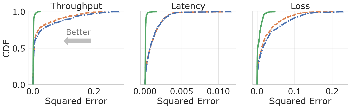
We evaluate CrystalBox using two input-driven environments: Adaptive Bitrate Streaming (ABR) and Congestion Control (CC). In ABR, the controller selects the video quality for an online stream presented to a user. The reward for the controller is the user’s quality of experience, quantified as a weighted sum of quality, quality change, and stalling. In CC, the controller manages the Internet traffic of a connection between a sender and a receiver by adjusting the sending rate of the sender. The reward here is a weighted sum of throughput, latency, and loss. ABR has discrete actions and CC has continuous actions.
We experiment with the publicly available ABR controller maguro (Patel et al. 2023) deployed on the Puffer Platform (Yan et al. 2020). It is the best ABR controller on Puffer. For Congestion Control, we borrow the DRL controller Aurora (Jay et al. 2019).
In all of our evaluations, we use a held-out set of traces . We use it to evaluate fidelity, controller performance, and network observability.
7.2 Fidelity Evaluation
We evaluate CrystalBox under two classes of actions: actions that the policy takes (factual actions), and actions that the policy does not take (counterfactual actions). That enables a wide range of explainability queries, including ‘Why A?’ and ‘Why A and not B?’. We compare predictions of CrystalBox with sampling techniques (§ 6.2) for each return component using the fidelity metric (§ 6.1).
In Figure 4, we show the error of returns predicted by CrystalBox and sampling baselines. We see that CrystalBox outperforms both of the sampling approaches in generating high-fidelity predictions for all three return components across both environments, under factual (Fig. 4(a), 4(c)) and counterfactual (Fig. 4(b), 4(d)) actions. Note that despite ABR’s discrete action space and CC’s continuous one, CrystalBox offers high-fidelity explanations in each case. We believe that this is due to CrystalBox’s estimates being unbiased by construction, unlike the ones from sampling baselines.
7.3 CrystalBox Analysis


We turn to present a closer analysis of CrystalBox, focusing on its inference latency and design choices.
Runtime Analysis. We analyze the efficiency of CrystalBox by looking at its output latency and contrasting it with sampling-based techniques. We find that in both ABR and CC, CrystalBox has a latency of less than ms, while sampling-based methods have a latency from ms to ms. Note that this low latency of CrystalBox enables real-time applications such as networking observability.
Joint Training Through an Auxiliary Loss Function. In designing CrystalBox, our priority was to avoid modifying the controller or its training process. This flexibility allows CrystalBox to work across various policies and environments without necessitating redesigns.
An immediate question that may arise is if modifying the agent could yield a better explainer. To explore this, we run an experiment where the controller and explainer are jointly trained without altering the controller’s training parameters. We optimize the RL algorithm’s loss and CrystalBox’s loss with a weighted sum. One may postulate this might enhance both the policy and the explainer (Lyle et al. 2021).
In Figure 6(a), we study the shared-training strategy of using a weighted joint loss function in congestion control. Increasing the weight for policy loss improves the policy’s quality to nearly match one trained without a predictor, but the quality of CrystalBox falls as anticipated (see orange dot). Conversely, if we increase the weight for CrystalBox, the policy quality drops and the predictor does not improve (see red dot). While this may be surprising, we hypothesize that such behavior should be expected. Recall that samples of are unbiased, but have high variance. Therefore, it requires a large number of samples to effectively learn. When we attempt to learn both a policy and a predictor simultaneously, we introduce an additional source of variance, with continuously changing with policy changes. As a result, devising a solution for joint training is highly non-trivial.
7.4 CrystalBox Applications
Lastly, we evaluate CrystalBox on concrete applications.
Network Observability. CrystalBox can assist an operator in observing system behavior by triggering potential performance degradation alerts. These alerts can help maintain online safety assurance (Rotman, Schapira, and Tamar 2020) and improve the controller.
Managing data large streams in observability is challenging, leading us to propose a post-processing mechanism. It utilizes a ‘threshold’ concept to demarcate boundaries for binary events. When a threshold is reached, an alert is triggered. Threshold values can be set based on risk and cost.
We assess the performance of our alert mechanism, treating alerts as event predictors in a binary classification problem. We rollout policy under the held-out trace set , considering two kinds of actions: the policy’s actions (factual) and alternative actions (counterfactual). Then, we observe if the threshold was reached for the state and action.
Figure 7 shows our results for ABR and CC under factual actions. Observing the ABR results, we note the following. CrystalBox exhibits high recall and low false-positive rates for both quality drops and long stalls in factual explanations. Sampling-based methods miss all long stalls but detect large quality changes better, albeit with higher false positives. These observations hold for the CC environment. Similar findings for counterfactual actions are in Appendix A.2.
Guiding Reward Design. Fine-tuning the weights of the reward function is a pain point for operators. CrystalBox can help in simplifying this process by letting us narrowly analyze their impact on specific scenarios.
Consider a scenario where the operator is troubleshooting the weights on the reward function of an ABR controller that reduces the bitrate even in seemingly ‘good’ states. To gain insight, we query CrystalBox for these states with two actions: the controller’s (where the bitrate drops) and a steady one continuing at the last bitrate. Then, we identify the dominant reward component that pushes the controller to deviate from steady action through the largest absolute difference between the two predicted decomposed future returns.
In Figure 5(a), we plot the frequency at which each reward component was found to be dominant. The operator first chooses a stall weight of 100 (leftmost bars) and observes that the stalling penalty dominates the decision-making process of the controller. This finding hints to the designer that the weight of the stalling penalty is too high and that they should try 25 (middle bars) or 10 (right bars) where the number of bitrate drops in such states is smaller, and less often motivated by the stalling reward component.
8 Discussion and Future Work
Prior work (Juozapaitis et al. 2019; Anderson et al. 2019) introduced a method to generate explanations based on a decomposed deep Q-learning technique for game environments and evaluated this idea on grid-world games. This approach is designed for Q-learning policies, and Q-learning cannot be applied to continuous control input-driven environments. Moreover, they assume access to and the ability to modify the training procedure. In contrast, our approach works for both discrete and continuous control systems without altering the training procedure.
Investigating the use of feature-based techniques for creating interpretable future return predictors represents a compelling research direction. Another potential avenue is to explore whether we can employ future return predictors during policy learning for human-in-the-loop frameworks.
References
- Anderson et al. (2019) Anderson, A.; Dodge, J.; Sadarangani, A.; Juozapaitis, Z.; Newman, E.; Irvine, J.; Chattopadhyay, S.; Fern, A.; and Burnett, M. 2019. Explaining reinforcement learning to mere mortals: An empirical study. arXiv preprint arXiv:1903.09708.
- Bastani, Pu, and Solar-Lezama (2018) Bastani, O.; Pu, Y.; and Solar-Lezama, A. 2018. Verifiable reinforcement learning via policy extraction. Advances in neural information processing systems, 31.
- Beattie et al. (2016) Beattie, C.; Leibo, J. Z.; Teplyashin, D.; Ward, T.; Wainwright, M.; Küttler, H.; Lefrancq, A.; Green, S.; Valdés, V.; Sadik, A.; et al. 2016. Deepmind lab. arXiv preprint arXiv:1612.03801.
- Brockman et al. (2016) Brockman, G.; Cheung, V.; Pettersson, L.; Schneider, J.; Schulman, J.; Tang, J.; and Zaremba, W. 2016. Openai gym. arXiv preprint arXiv:1606.01540.
- Browne et al. (2012) Browne, C. B.; Powley, E.; Whitehouse, D.; Lucas, S. M.; Cowling, P. I.; Rohlfshagen, P.; Tavener, S.; Perez, D.; Samothrakis, S.; and Colton, S. 2012. A survey of monte carlo tree search methods. IEEE Transactions on Computational Intelligence and AI in games, 4(1): 1–43.
- Burkart and Huber (2021) Burkart, N.; and Huber, M. F. 2021. A survey on the explainability of supervised machine learning. Journal of Artificial Intelligence Research, 70: 245–317.
- Chen et al. (2018) Chen, L.; Lingys, J.; Chen, K.; and Liu, F. 2018. Auto: Scaling deep reinforcement learning for datacenter-scale automatic traffic optimization. In Proceedings of the 2018 conference of the ACM special interest group on data communication, 191–205.
- Cruz et al. (2021) Cruz, F.; Dazeley, R.; Vamplew, P.; and Moreira, I. 2021. Explainable robotic systems: Understanding goal-driven actions in a reinforcement learning scenario. Neural Computing and Applications, 1–18.
- Doshi-Velez et al. (2017) Doshi-Velez, F.; Kortz, M.; Budish, R.; Bavitz, C.; Gershman, S.; O’Brien, D.; Scott, K.; Schieber, S.; Waldo, J.; Weinberger, D.; et al. 2017. Accountability of AI under the law: The role of explanation. arXiv preprint arXiv:1711.01134.
- Greydanus et al. (2018) Greydanus, S.; Koul, A.; Dodge, J.; and Fern, A. 2018. Visualizing and understanding atari agents. In International conference on machine learning, 1792–1801. PMLR.
- Holkar and Waghmare (2010) Holkar, K.; and Waghmare, L. M. 2010. An overview of model predictive control. International Journal of control and automation, 3(4): 47–63.
- Iyer et al. (2018) Iyer, R.; Li, Y.; Li, H.; Lewis, M.; Sundar, R.; and Sycara, K. 2018. Transparency and explanation in deep reinforcement learning neural networks. In Proceedings of the 2018 AAAI/ACM Conference on AI, Ethics, and Society, 144–150.
- Jay et al. (2019) Jay, N.; Rotman, N.; Godfrey, B.; Schapira, M.; and Tamar, A. 2019. A deep reinforcement learning perspective on internet congestion control. In International conference on machine learning, 3050–3059. PMLR.
- Juozapaitis et al. (2019) Juozapaitis, Z.; Koul, A.; Fern, A.; Erwig, M.; and Doshi-Velez, F. 2019. Explainable reinforcement learning via reward decomposition. In IJCAI/ECAI Workshop on explainable artificial intelligence.
- Krishnan et al. (2018) Krishnan, S.; Yang, Z.; Goldberg, K.; Hellerstein, J.; and Stoica, I. 2018. Learning to optimize join queries with deep reinforcement learning. arXiv preprint arXiv:1808.03196.
- Langley et al. (2017) Langley, A.; Riddoch, A.; Wilk, A.; Vicente, A.; Krasic, C.; Zhang, D.; Yang, F.; Kouranov, F.; Swett, I.; Iyengar, J.; et al. 2017. The quic transport protocol: Design and internet-scale deployment. In Proceedings of the conference of the ACM special interest group on data communication, 183–196.
- Lyle et al. (2021) Lyle, C.; Rowland, M.; Ostrovski, G.; and Dabney, W. 2021. On the effect of auxiliary tasks on representation dynamics. In International Conference on Artificial Intelligence and Statistics, 1–9. PMLR.
- Mao et al. (2019) Mao, H.; Negi, P.; Narayan, A.; Wang, H.; Yang, J.; Wang, H.; Marcus, R.; Khani Shirkoohi, M.; He, S.; Nathan, V.; et al. 2019. Park: An open platform for learning-augmented computer systems. Advances in Neural Information Processing Systems, 32.
- Mao, Netravali, and Alizadeh (2017) Mao, H.; Netravali, R.; and Alizadeh, M. 2017. Neural adaptive video streaming with pensieve. In Proceedings of the Conference of the ACM Special Interest Group on Data Communication, 197–210.
- Mao et al. (2018) Mao, H.; Venkatakrishnan, S. B.; Schwarzkopf, M.; and Alizadeh, M. 2018. Variance reduction for reinforcement learning in input-driven environments. arXiv preprint arXiv:1807.02264.
- Meng et al. (2020) Meng, Z.; Wang, M.; Bai, J.; Xu, M.; Mao, H.; and Hu, H. 2020. Interpreting deep learning-based networking systems. In Proceedings of the Annual conference of the ACM Special Interest Group on Data Communication on the applications, technologies, architectures, and protocols for computer communication, 154–171.
- Miller (2019) Miller, T. 2019. Explanation in artificial intelligence: Insights from the social sciences. Artificial intelligence, 267: 1–38.
- Mittelstadt, Russell, and Wachter (2019) Mittelstadt, B.; Russell, C.; and Wachter, S. 2019. Explaining explanations in AI. In Proceedings of the conference on fairness, accountability, and transparency, 279–288.
- Mnih et al. (2013) Mnih, V.; Kavukcuoglu, K.; Silver, D.; Graves, A.; Antonoglou, I.; Wierstra, D.; and Riedmiller, M. 2013. Playing atari with deep reinforcement learning. arXiv preprint arXiv:1312.5602.
- Mok, Chan, and Chang (2011) Mok, R. K.; Chan, E. W.; and Chang, R. K. 2011. Measuring the quality of experience of HTTP video streaming. In 12th IFIP/IEEE International Symposium on Integrated Network Management (IM 2011) and Workshops, 485–492. IEEE.
- Patel, Abdu Jyothi, and Narodytska (2024) Patel, S.; Abdu Jyothi, S.; and Narodytska, N. 2024. CrystalBox: Future-Based Explanations for Input-Driven Deep RL Systems. Proceedings of the AAAI Conference on Artificial Intelligence, 38(13): 14563–14571.
- Patel et al. (2023) Patel, S.; Zhang, J.; Jyothi, S. A.; and Narodytska, N. 2023. Plume: A Framework for High Performance Deep RL Network Controllers via Prioritized Trace Sampling. arXiv:2302.12403.
- Pohlen et al. (2018) Pohlen, T.; Piot, B.; Hester, T.; Azar, M. G.; Horgan, D.; Budden, D.; Barth-Maron, G.; Van Hasselt, H.; Quan, J.; Večerík, M.; et al. 2018. Observe and look further: Achieving consistent performance on atari. arXiv preprint arXiv:1805.11593.
- Puri et al. (2019) Puri, N.; Verma, S.; Gupta, P.; Kayastha, D.; Deshmukh, S.; Krishnamurthy, B.; and Singh, S. 2019. Explain your move: Understanding agent actions using specific and relevant feature attribution. arXiv preprint arXiv:1912.12191.
- Ribeiro, Singh, and Guestrin (2016) Ribeiro, M. T.; Singh, S.; and Guestrin, C. 2016. ” Why should i trust you?” Explaining the predictions of any classifier. In Proceedings of the 22nd ACM SIGKDD international conference on knowledge discovery and data mining, 1135–1144.
- Rotman, Schapira, and Tamar (2020) Rotman, N. H.; Schapira, M.; and Tamar, A. 2020. Online safety assurance for learning-augmented systems. In Proceedings of the 19th ACM Workshop on Hot Topics in Networks, 88–95.
- Silver (2015) Silver, D. 2015. Lectures on Reinforcement Learning. https://www.davidsilver.uk/teaching/. Accessed: 2022-10-12.
- Sutton and Barto (2018) Sutton, R. S.; and Barto, A. G. 2018. Reinforcement learning: An introduction. MIT press.
- van der Waa et al. (2018) van der Waa, J.; van Diggelen, J.; Bosch, K. v. d.; and Neerincx, M. 2018. Contrastive explanations for reinforcement learning in terms of expected consequences. arXiv preprint arXiv:1807.08706.
- Verma et al. (2018) Verma, A.; Murali, V.; Singh, R.; Kohli, P.; and Chaudhuri, S. 2018. Programmatically interpretable reinforcement learning. In International Conference on Machine Learning, 5045–5054. PMLR.
- Yan et al. (2020) Yan, F. Y.; Ayers, H.; Zhu, C.; Fouladi, S.; Hong, J.; Zhang, K.; Levis, P.; and Winstein, K. 2020. Learning in situ: a randomized experiment in video streaming. In 17th USENIX Symposium on Networked Systems Design and Implementation (NSDI 20), 495–511.
- Yau, Russell, and Hadfield (2020) Yau, H.; Russell, C.; and Hadfield, S. 2020. What did you think would happen? explaining agent behaviour through intended outcomes. Advances in Neural Information Processing Systems, 33: 18375–18386.
- Zahavy, Ben-Zrihem, and Mannor (2016) Zahavy, T.; Ben-Zrihem, N.; and Mannor, S. 2016. Graying the black box: Understanding dqns. In International conference on machine learning, 1899–1908. PMLR.
- Zhang, Zhou, and Lin (2020) Zhang, H.; Zhou, A.; and Lin, X. 2020. Interpretable policy derivation for reinforcement learning based on evolutionary feature synthesis. Complex & Intelligent Systems, 6(3): 741–753.


Appendix A Appendix
A.1 Traces
In this section, we visualize representative traces in Figure 10 and Figure 11 for ABR and CC applications, respectively.
In ABR, a trace is the over-time throughput of the internet connection between a viewer and a streaming platform. We obtain a representative set of traces by analyzing the logged data of a public live-streaming platform (Yan et al. 2020). In Figure 10 we present a visualization of a few of those traces for the first 100 seconds. Note that the y-axis is different on each plot due to inherent differences between traces. However, even with the naked eye, we can see that some traces are high-throughput traces, e.g. all traces in the third row, while other traces are slow-throughput, e.g. the first plot in the second row. To further analyze these inherent differences, we analyze the distribution of mean and coefficient of variance of throughput within each trace. In Figure 12, we see that a majority of traces have high mean throughput. When we analyze this jointly with the distribution of the throughput coefficient of variance, we see that a majority of those traces also have smaller variances. Only a small number of traces represent poor network conditions such as low throughput or high throughput variance. These observations are consistent with a recent Google study (Langley et al. 2017) that showed that more than of YouTube streams never come to a stall.
In CC, a trace is the over-time network conditions between a sender and receiver. We obtain a representative set of traces by following (Jay et al. 2019) and synthetically generating them by four key values: mean throughput, latency, queue size, and loss rate. In Figure 11, we demonstrate how these traces may look like from the sender’s perspective by looking at the effective throughput over time. Similar to the traces in ABR, we can visually see that the traces can be greatly different from one another. In Figure 13, we analyze the effective distribution of these traces. We observe that while the distribution is not nearly as unbalanced as it is in ABR, there are still only a small number of traces that have exceedingly harsh network conditions.
A.2 Network Observability (Counterfactual actions)
We present the performance of CrystalBox for network observability by analyzing its ability to rise alerts about upcoming large performance drops under counterfactual actions. We recall that our goal is to detect states and actions that lead to large performance drops. We employ CrystalBox’s optional post-processing and convert vectors of output values into binary events. In our experiments, we used the following thresholds. For ABR, we used: quality return below 0.55, quality change return below -0.1, and stalling return below -0.25. For CC, we used: throughput return below 0.3, latency return below -0.075, and loss return below -0.1.
In Section 7.4, we analyzed the performance of CrystalBox’s ability to detect these events under factual actions (actions that the policy takes). Now, we turn to present the results of the same state under comparative counterfactual actions. In Figure 9, we present the recall and false-positive rates of different return predictors. Similar to the results under factual actions, we find that CrystalBox has higher recall and lower false-positive rates. In ABR, we see that CrystalBox achieves significantly higher recall in detecting quality drop and stalling events while having about higher false-positive rates. We additionally see that Distribution-Aware sampling achieves significantly higher recall than Naive sampling, particularly in long stall events. In CC, we see that CrystalBox is particularly adept at detecting throughput drop and high latency events, but suffers from high false-positive rates of high loss events.
A.3 Fidelity Evaluation (additional results)
We present our evaluation of CrystalBox explanations on all traces. Figure 8 shows our results. We can see that all predictors perform well. For high throughput traces, the optimal policy for the controller is simple: send the highest bitrate. Therefore, all predictors do well on these traces. However, the relative performance between the predictors is the same as it was with traces that could experience stalling and quality drops 4. The CrystalBox outperforms sampling-based methods across all three reward components under both factual and counterfactual actions.
A.4 Policy Rollouts
We collect samples of the ground truth values of the decomposed future returns by rolling out the policy in a simulation environment. That is, we let the policy interact with the environment under an offline set of traces , and observe sequences of the tuple . With these tuples, we can calculate the decomposed return for each timestamp. In practice, we do not use an infinite sum to obtain . This is because the variance of this function can be close to infinity due to its dependence on the length of , which can range from 1 to infinity (Mao et al. 2018). Instead, we bound this sum by a constant . This approximates with a commonly used truncated version where the rewards after are effectively zero (Sutton and Barto 2018).
For a given episode, these states and returns can be highly correlated (Mnih et al. 2013). Thus, to efficiently cover a wide variety of scenarios, we do not consider the states and returns after for steps. Moreover, when attempting to collect samples for a counterfactual action , we ensure the rewards and actions from timestamp onwards are not used in the calculation for any state-action pair before . This strategy avoids adding any additional noise to samples of due to exploratory actions.
is a hyper-parameter for each environment. In systems environments, we usually observe the effect of each action within a short time horizon. For example, if a controller drops bitrate, then the user experiences lower quality video in one step. Therefore, it is only required to consider rollouts of a few steps to capture the consequences of each action, so of five is sufficient for our environments.
A.5 CrystalBox Details
Preprocessing. We employ Monte Carlo Rollouts to get samples of for training our learned predictor. By themselves, the return components can vary across multiple orders of magnitude. Thus, similar to the standard reward clipping (Mnih et al. 2013) and return normalization (Pohlen et al. 2018) techniques widely employed in Q-learning, we normalize all the returns to be in the range [0, 1].
Neural Architecture Design. We design the neural architecture of our learned predictors to be compact and sample efficient. We employ shared layers that feed into separate fully connected ‘tails’ that then predict the return components. We model the samples of as samples from a Gaussian distribution and predict the parameters (mean and standard deviation) to this distribution in each tail. To learn to predict these parameters, we minimize the negative log-likelihood loss of each sample of .
For the fully connected layers, we perform limited tuning to choose the units of these layers from {64, 128, 256, 512}. We found that a smaller number of units is enough in both of our environments. We present a visualization of our architectures in Figures 14 and 15.
Learning Parameters. We learn our predictors in two stages. In the first stage, we train our network end-to-end. In the second stage, we freeze the shared weights in our network and fine-tune our predictors with a smaller learning rate. We use an Adagrad optimizer, and experimented with learning rates from 1e-6 to 1e-4, with decay from 1e-10 to 1e-9. We tried batch sizes from {50, 64, 128, 256, 512}. We found that small batch sizes, learning rates, and decay work best.