Cross-Layer Feature Pyramid Transformer for Small Object Detection in Aerial Images
Abstract
Object detection in aerial images has always been a challenging task due to the generally small size of the objects. Most current detectors prioritize novel detection frameworks, often overlooking research on fundamental components such as feature pyramid networks. In this paper, we introduce the Cross-Layer Feature Pyramid Transformer (CFPT), a novel upsampler-free feature pyramid network designed specifically for small object detection in aerial images. CFPT incorporates two meticulously designed attention blocks with linear computational complexity: the Cross-Layer Channel-Wise Attention (CCA) and the Cross-Layer Spatial-Wise Attention (CSA). CCA achieves cross-layer interaction by dividing channel-wise token groups to perceive cross-layer global information along the spatial dimension, while CSA completes cross-layer interaction by dividing spatial-wise token groups to perceive cross-layer global information along the channel dimension. By integrating these modules, CFPT enables cross-layer interaction in one step, thereby avoiding the semantic gap and information loss associated with element-wise summation and layer-by-layer transmission. Furthermore, CFPT incorporates global contextual information, which enhances detection performance for small objects. To further enhance location awareness during cross-layer interaction, we propose the Cross-Layer Consistent Relative Positional Encoding (CCPE) based on inter-layer mutual receptive fields. We evaluate the effectiveness of CFPT on two challenging object detection datasets in aerial images, namely VisDrone2019-DET and TinyPerson. Extensive experiments demonstrate the effectiveness of CFPT, which outperforms state-of-the-art feature pyramid networks while incurring lower computational costs. The code will be released at https://github.com/duzw9311/CFPT.
Index Terms:
Aerial image, object detection, feature pyramid network, vision transformer.I Introduction
Benefiting from advancements in Convolutional Neural Networks (CNNs) and Vision Transformers (ViTs), existing object detectors have made significant progress, establishing themselves as fundamental solutions across various applications, including autonomous driving, face detection, medical image analysis, and industrial quality inspection.
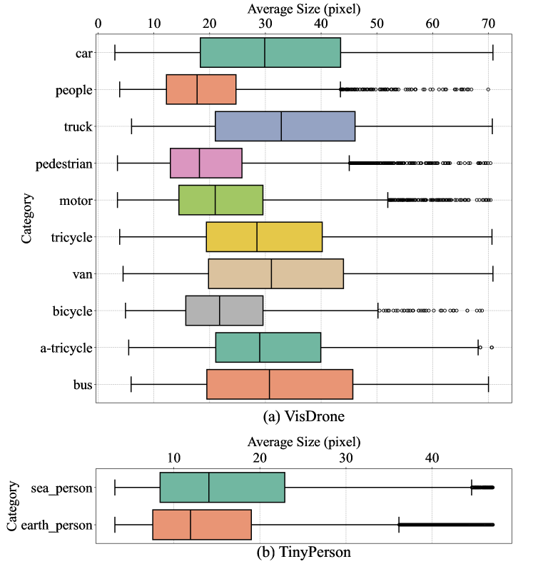
As a subfield of object detection, small object detection still faces greater challenges than traditional object detection tasks due to the features of small objects being lost or overshadowed by the features of larger objects during the convolution and pooling operations. As shown in Fig.3, we present box plots illustrating the data distribution of two classic small object detection datasets in aerial images: VisDrone2019-DET [2] and TinyPerson [3]. The box plot highlights that the VisDrone2019-DET dataset not only contains a substantial number of small objects (20 to 30 pixels) but also exhibits significant scale variations. In contrast, the TinyPerson dataset contains predominantly smaller objects compared to VisDrone2019-DET, with most objects being less than 20 pixels in size. The flying height and shooting angle of the drone significantly influence the scale distribution of objects, leading to relatively poorer performance of object detection on aerial images.
To address these challenges, numerous studies have been proposed consecutively. Given the small proportion of foreground in drone scenes, existing solutions typically adopt a coarse-to-fine detection scheme [4, 5, 6]. In the coarse prediction stage, a common detector is typically used to detect objects and predict dense object clusters. Subsequently, in the refinement stage, the cluster is usually pruned, upsampled, and re-inputted into the detector for a refined search. Although the above model architecture can effectively adapt to drone perspectives and enhance the performance of various detectors at a lower computational cost compared to directly inputting high-resolution images, it still lacks essential components tailored for object detection in aerial images, such as the feature pyramid network.
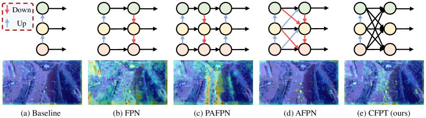
Feature pyramid networks, serving as a low-computation alternative to image pyramids, are extensively utilized in diverse detectors and have become one of the essential components of each detector. The earliest FPN [7] uses a top-down unidirectional path to integrate semantic information into shallow feature maps, effectively enhancing the model’s capabilities in multi-scale object detection. Since the single-directional paths transmitted layer by layer inevitably cause information loss [8], subsequent feature pyramid networks gradually transition to direct interaction between layers [9, 10, 11]. However, these structures are typically designed for detecting objects at common scales and often lack domain adaptability. Specifically, they typically employ static kernels to process all spatial points of multi-scale feature maps, which is suboptimal for scenes with significant scale variations, as objects of the same category may receive supervision signals across different scales of feature maps. Moreover, employing uniform operations across feature maps of varying scales is not the optimal approach for object detection tasks in aerial images that involve numerous small objects.
In this paper, we propose a novel feature pyramid network for small object detection in aerial images, named Cross-Layer Feature Pyramid Transformer (CFPT). As shown in Fig. 2, CFPT is upsampler-free, which can avoid the extra computation and memory usage caused by upsampling to improve computational efficiency. CFPT consists of two meticulously designed transformer blocks, namely Cross-layer Channel-wise Attention (CCA) and Cross-layer Spatial-wise Attention (CSA). CCA conducts cross-layer feature interactions along the channel dimension, while CSA conducts cross-layer feature interactions along the spatial dimension. By integrating these two modules, the model can achieve cross-layer information transfer in a single step, thereby reducing performance degradation due to semantic gaps and minimizing information loss associated with layer-by-layer propagation. Furthermore, CFPT effectively integrates global contextual information critical for small objects and prioritizes shallow feature maps rich in small objects through cross-scale neighboring interactions, capabilities that are typically unachievable with traditional FPNs. In addition, to enhance the model’s position awareness in capturing global contextual information, we propose Cross-layer Consistent Relative Positional Encoding (CCPE), enabling the model to leverage position priors of spatial and channel points across layers for deriving more accurate affinity matrices [13].
Our contributions can be summarized as follows.
-
•
We propose CFPT, a novel upsampler-free feature pyramid network for small object detection in aerial images. CFPT can accomplish multi-scale feature interactions in a single step and explicitly provide more attention to shallow feature maps through cross-layer neighborhood interaction groups, achieving lossless information transfer while introducing local inductive bias.
-
•
We propose two cross-layer attention blocks with linear computational complexity, named CCA and CSA, which facilitate cross-layer information interaction in distinct directions (i.e., spatial-wise and channel-wise). By integrating both, CFPT can effectively capture the necessary global contextual information for small object while maintaining lower computational costs.
-
•
We propose CCPE, a new positional encoding based on inter-layer mutual receptive fields, designed to enhance the model’s awareness of spatial and channel positions during cross-layer interactions.
-
•
Through extensive experiments on the VisDrone2019-DET and TinyPerson datasets, we demonstrate the effectiveness of CFPT for small object detection in aerial images.
II Related Work
II-A Small Object Detection in Aerial Images
Modern object detectors typically decrease the resolution of the input image through successive layers of convolution and pooling, striving to achieve an optimal balance between performance and computational complexity [14, 15, 16]. Therefore, detecting small objects is inherently more challenging than common object detection, as their diminutive size increases the risk of information loss during downsampling.
For small object detection in aerial images, ClusDet [17] employs a coarse-to-fine scheme that initially detects dense object clusters and then refines the search within these clusters to enhance the model’s ability to detect small objects. DMNet [18] simplifies the training process of ClusDet by employing a density map generation network to produce density maps for cluster prediction. Following the similar detection pipeline, CRENet [19] and GLSAN [4] further enhance the clustering prediction algorithm and optimize the fine-grained prediction scheme. UFPMP-Det [6] employs the UFP module and MP-Net to predict sub-regions, assembling them into a single image for efficient single-inference, thereby achieving improved detection accuracy and efficiency. CEASC [20] utilizes sparse convolution to optimize conventional detectors for object detection in aerial images, reducing computational requirements while maintaining competitive performance. DTSSNet [21] introduces a manually designed block between the Backbone and Neck to enhance the model’s sensitivity to multi-scale features and incorporates a training sample selection method specifically for small objects.
The above solutions optimize various detectors for object detection scenarios in aerial images, whereas we propose a new feature pyramid network specifically tailored for small object detection in this context.
II-B Feature Pyramid Network
To alleviate the substantial computational costs of image pyramids, feature pyramid networks (FPNs) have emerged as an effective and efficient alternative that enhances the performance of various detectors. FPN [7] utilizes a series of top-down shortcut branches to augment the semantic information lacking in shallow feature maps. Based on FPN, PAFPN [12] proposes using bottom-up shortcut branches to address the deficiency of detailed information in deep feature maps. Libra-RCNN [22] refines original features by incorporating non-local blocks to obtain balanced interactive features. To mitigate the semantic gap in multi-scale feature maps, AugFPN [23] introduces the consistent supervision branch and proposes ASF for dynamic feature integration across multiple scales. FPG [8] represents the feature scale space using a regular grid fused with multi-directional lateral connections between parallel paths, thereby enhancing the model’s feature representation. AFPN [11] iteratively refines multi-scale features through cross-level fusion of deep and shallow feature maps, achieving competitive performance in object detection with common scale distribution.
Distinct from previous approaches, we propose CFPT, which leverages global contextual information and strategically emphasizes shallow feature maps to enhance the detection of small objects in aerial images.
II-C Vision Transformer
As an extension of Transformer [24] in computer vision, Vision Transformer (ViT) [25] have demonstrated significant potential across various visual scenarios [26, 27, 28]. Due to the quadratic computational complexity of conventional ViTs with respect to image resolution, subsequent research has predominantly focused on developing lightweight alternatives. Swin Transformer [29] restricts interactions to specific windows and achieves a global receptive field by shifting these windows during the interaction process. Local ViTs [30, 31, 32] incorporate local inductive bias through interactions within local windows, effectively reducing the model’s computational complexity and accelerating its convergence speed. Axial Attention [33] reduces computational complexity by confining interactions to strips along the width and height of the image.
Following the similar lightweight concept, we design two attention blocks with linear complexity (i.e., CCA and CSA) to capture the global contextual information across layers along various directions (i.e., spatial-wise and channel-wise), thereby enhancing the model’s ability to detect small objects.
III Methodology
In this section, we will provide a detailed introduction to the proposed Cross-layer Feature Pyramid Transformer (CFPT). In Section III-A, we first outline the overall architecture of proposed CFPT. Subsequently, in Section III-B and Section III-C, we introduce the two key components of CFPT, namely the Cross-layer Channel-wise Attention (CCA) and the Cross-layer Spatial-wise Attention (CSA). In Section III-D, we present a novel Cross-layer Consistent Relative Positional Encoding (CCPE) designed to enhance the model’s cross-layer position-aware capability.
III-A Overview
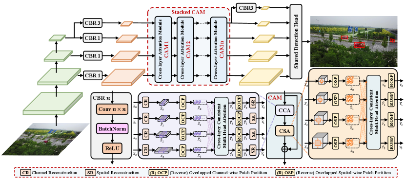
As illustrated in Fig. 4, CFPT employs multiple parallel CBR blocks to construct the input for cross-layer feature interaction using the multi-level feature map outputs from the feature extraction network (e.g., ResNet[34]), thereby reducing computational complexity and meeting the architectural requirements of most detectors. By leveraging stacked Cross-layer Attention Modules (CAMs), CFPT is able to enhance the model’s ability to utilize both global contextual information and cross-layer multi-scale information.
Specifically, the CAM module consists of a sequence of Cross-layer Channel-wise Attention (CCA) and Cross-layer Spatial-wise Attention (CSA). The CCA facilitates local cross-layer interactions along the channel dimension, consequently establishing a global receptive field along the spatial dimension through interactions within each channel-wise token group. Conversely, CSA facilitates local cross-layer interactions along the spatial dimension, capturing global contextual information along the channel dimension through interactions within each spatial-wise token group. In addition, we further improve the gradient gain by using shortcut branches between input and output of CAM.
Assume that the feature map of each scale after the CBR block can be represented as , where is the number of input layers, and the spatial resolution of each feature map increases with while maintaining the same number of channels . The above process can be described as
| (1) |
where is a set of multi-scale feature maps after cross-layer interaction, maintaining the same shape as the corresponding input feature maps.
It is noteworthy that our CFPT eliminates the complex feature upsampling operations and layer-by-layer information transmission mechanisms, which are prone to information loss during inter-layer transmission and contribute to increased computational load and memory access delays. Instead, we perform a local grouping operation on multi-scale feature maps by utilizing the mutual receptive field size between scales, and subsequently facilitate information mixing between scales through a one-step cross-layer neighboring interaction operation. This approach enables features at each scale to acquire information from other layers in a balanced manner (even if the layers are distant) while facilitating self-correction and benefiting from the inductive bias provided by local interactions [32].
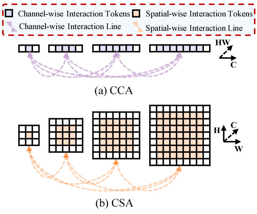
III-B Cross-layer Channel-wise Attention
Suppose the set of input feature maps of the CCA is . As shown in Fig. 5(a), CCA executes multi-scale neighboring interactions across layers along the channel dimension, thereby furnishing global contextual information along the spatial dimension for each channel-wise token. To construct the interactive input, we first perform Channel Reconstruction (CR) on the feature map of each scale to ensure they have the same spatial resolution, thereby obtaining . CR is an operator similar to Focus in YOLOv5, but it differs in that it does not use additional operations for feature mapping. Instead, CR stacks feature values from the spatial dimension into the channel dimension, thereby achieving consistent spatial resolution while maintaining efficiency. The above process can be described as
| (2) |
Next, we perform the Overlapped Channel-wise Patch Partition (OCP) to form channel-wise token groups, which can be viewed as the Patch Embedding [25] with overlapping regions in local areas along the channel dimension, where the patch sizes vary for feature maps at different scales. Specifically, according to the shape of multi-scale features, the channel sizes of adjacent feature maps in differ by a factor of (i.e., ). To construct overlapping neighboring interaction groups, we introduce an expansion factor to perform OCP on , resulting in . The above process can be described as
| (3) |
Taking the feature map of the -th layer as an example, after obtaining , we employ the cross-layer consistent multi-head attention to capture the global dependencies along the spatial dimension, thereby obtaining the interaction result .
| (4) | ||||
| (5) |
where are the linear projection matrices. and represent the concatenated keys and values, respectively, where represents concatenation operation. denotes the -th Cross-layer Consistent Relative Positional Encoding (CCPE), with details will be introduced in Section III-D. Note that for simplicity, we only consider the case where the number of heads is . In practice, we employ the multi-head mechanism to capture global dependencies for each channel-wise token.
After obtaining the interaction results for feature maps at each scale, we apply the Reverse Overlapped Channel-wise Patch Partition (ROCP) to restore the impact of OCP and obtain . As the reverse operation of OCP, ROCP aims to restore the original spatial resolution using the same kernel size and stride as OCP.
Finally, we use Spatial Reconstruction (SR) to obtain the result that matches the shape of the input .
| (6) |
III-C Cross-layer Spatial-wise Attention
Similarly, let the set of input feature maps for the CSA be denoted as . As illustrated in Fig. 5(b), CSA performs multi-scale neighboring interactions across layers along the spatial dimension, providing global contextual information along the channel dimension for each spatial-wise token.
Since the channel sizes of the input feature maps are matched after the CBR block(e.g., 256), there is no need to align their sizes using methods such as CR and SR, as is done in CCA. Therefore, we can directly perform Overlapped Spatial-wise Patch Partition (OSP) to form spatial-wise token groups, which can be viewed as sliding crops on feature maps of different scales using rectangular boxes of varying sizes. Suppose the expansion factor for OSP is , through the above operation, we can get . The above process can be expressed as
| (7) |
Then, we can perform local interaction within cross-layer spatial-wise token groups and use the cross-layer consistent multi-head attention to capture global dependencies along the channel dimension, thereby obtaining . For the feature map of the -th layer, this process can be expressed as follows:
| (8) | ||||
| (9) |
where are the linear projection matrices. and . denotes the Cross-layer Consistent Relative Positional Encoding (CCPE) for the -th layer.
Next, we employ Reverse Overlapped Spatial Patch Partition (ROSP) to reverse the effect of OSP and obtain the interaction result set .
| (10) |
III-D Cross-layer Consistent Relative Positional Encoding
Since each token within their cross-layer token groups maintains specific positional relationships during the interaction process. However, the vanilla multi-head attention treats all interaction tokens uniformly, resulting in suboptimal results for position-sensitive tasks such as object detection. Therefore, we introduce Cross-layer Consistent Relative Positional Encoding (CCPE) to enhance the cross-layer location awareness of CFPT during the interaction process.
The main solution of CCPE is based on aligning mutual receptive fields across multiple scales, which is determined by the properties of convolution. Taking CSA as an example, the set of attention maps between each spatial-wise token group can be expressed as , where is the number of heads and , as defined in Equation 9. For simplicity, we ignore and and define and , where and represent the height and width of the spatial-wise token groups in the -th and -th layers. Therefore, the set of attention maps can be re-expressed as .
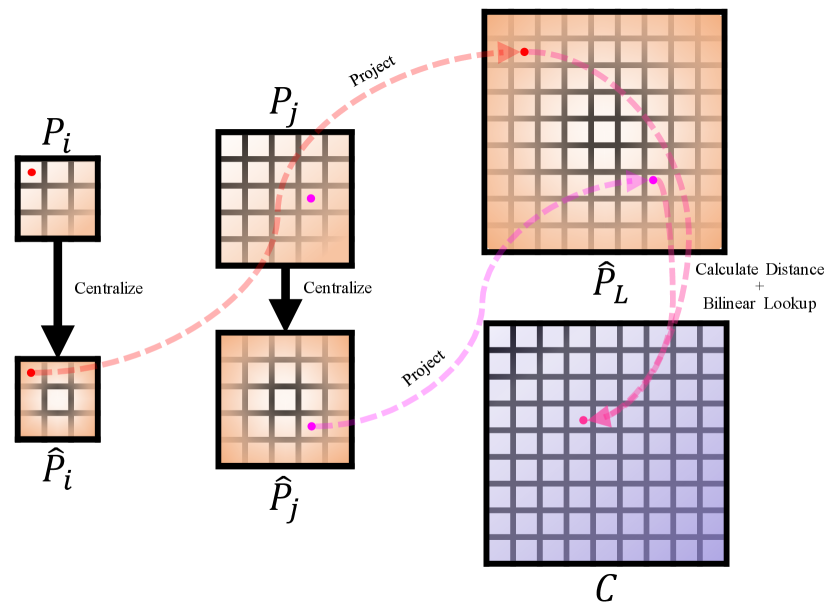
The process of CCPE is shown Fig. 6. We define a learnable codebook and obtain the relative position information between any two tokens from the codebook by calculating their cross-layer consistent relative position index. For simplicity, consider the interaction of the spatial-wise token groups from the -th and -th layers, where and represent their respective absolute coordinate matrices.
| (11) |
To obtain the relative position information of relative to , we first centralize their coordinates using their respective spatial-wise token group sizes to obtain and .
| (12) |
Then we can derive and by projecting their coordinates to the largest spatial-wise token group.
| (13) |
Subsequently, we can calculate the relative distance between and and convert the relative distance into the index of the codebook.
| (14) |
Finally, we extract the corresponding positional embedding vector from the codebook using the index and superimpose it on the original attention map , resulting in the output with enhanced positional information.
| (15) |
where is the bilinear interpolation function used to ensure the differentiability when extracting relative positional information from the codebook using non-integer coordinates derived from Equation 13, with representing the codebook and denoting the non-integer coordinates matrix.
III-E Complexity Analysis
In this section, we will analyze the computational complexity of both CCA and CSA. In addition, since the sizes of the spatial-wise and channel-wise token groups remain constant during both training and testing phases, their computational complexity scales linearly with the spatial resolution of the input feature maps.
III-E1 Cross-layer Channel-wise Attention
Consider a set of input feature maps denoted as . Additionally, let denote the expansion factor used in CCA. The overall computational complexity of CCA includes for linear projections, for attention interactions, and for FFNs.
III-E2 Cross-layer Spatial-wise Attention
Suppose the set of input feature maps is . Additionally, let denote the expansion factor used in CSA. The overall computational complexity of CSA includes for linear projections, for attention interactions, and for FFNs.
| Method | Backbone | AP(%) | AP0.5(%) | AP0.75(%) | AP-small(%) | AP-medium(%) | AP-large(%) | Params(M) | FLOPs(G) |
|---|---|---|---|---|---|---|---|---|---|
| RetinaNet [1] | ResNet-18 | 15.8 | 28.4 | 15.6 | 7.5 | 24.4 | 33.2 | 18.0 | 151.1 |
| FPN [7] | ResNet-18 | 18.1 | 32.7 | 17.8 | 9.2 | 28.7 | 33.6 | 19.8 | 164.0 |
| PAFPN [12] | ResNet-18 | 18.2 | 32.5 | 18.2 | 8.9 | 28.9 | 36.3 | 22.2 | 170.1 |
| AugFPN [23] | ResNet-18 | 18.6 | 33.2 | 18.4 | 9.0 | 29.5 | 37.3 | 20.4 | 164.2 |
| DRFPN [35] | ResNet-18 | 18.9 | 33.4 | 18.8 | 9.1 | 30.2 | 38.5 | 24.6 | 176.0 |
| FPG [8] | ResNet-18 | 18.6 | 33.2 | 18.4 | 9.5 | 29.6 | 36.0 | 58.1 | 290.5 |
| FPT | ResNet-18 | 17.5 | 30.7 | 17.5 | 8.3 | 28.0 | 37.9 | 40.1 | 275.2 |
| RCFPN [36] | ResNet-18 | 18.3 | 32.4 | 18.1 | 8.6 | 29.3 | 36.3 | 23.0 | 157.5 |
| SSFPN [37] | ResNet-18 | 19.2 | 33.7 | 19.1 | 10.0 | 31.2 | 35.8 | 24.3 | 221.4 |
| AFPN [11] | ResNet-18 | 16.5 | 30.0 | 16.5 | 8.2 | 26.0 | 32.3 | 17.9 | 153.2 |
| CFPT (ours) | ResNet-18 | 20.0 | 35.3 | 20.0 | 10.1 | 31.7 | 37.2 | 20.8 | 165.9 |
| RetinaNet [1] | ResNet-50 | 18.1 | 31.1 | 18.3 | 8.8 | 28.5 | 38.0 | 34.5 | 203.7 |
| FPN [7] | ResNet-50 | 21.0 | 36.4 | 21.4 | 10.9 | 34.3 | 40.1 | 36.3 | 216.6 |
| PAFPN [12] | ResNet-50 | 21.2 | 36.5 | 21.6 | 10.9 | 34.6 | 41.1 | 38.7 | 222.7 |
| AugFPN [23] | ResNet-50 | 21.7 | 37.1 | 22.2 | 11.1 | 35.4 | 40.4 | 38.1 | 216.8 |
| DRFPN [35] | ResNet-50 | 21.5 | 36.7 | 22.0 | 11.0 | 35.3 | 39.5 | 41.1 | 228.5 |
| FPG [8] | ResNet-50 | 21.7 | 37.3 | 22.2 | 11.5 | 35.2 | 38.7 | 71.0 | 346.1 |
| FPT [10] | ResNet-50 | 19.3 | 33.3 | 19.2 | 9.4 | 30.0 | 38.9 | 56.6 | 331.8 |
| RCFPN [36] | ResNet-50 | 21.0 | 36.0 | 21.3 | 10.5 | 34.8 | 38.1 | 36.0 | 209.2 |
| SSFPN [37] | ResNet-50 | 21.7 | 37.3 | 22.2 | 11.5 | 35.3 | 39.8 | 40.8 | 274.0 |
| AFPN [11] | ResNet-50 | 20.7 | 36.0 | 21.2 | 10.7 | 33.4 | 36.9 | 58.0 | 250.0 |
| CFPT (ours) | ResNet-50 | 22.2 | 38.0 | 22.4 | 11.9 | 35.2 | 41.7 | 37.3 | 218.5 |
| RetinaNet [1] | ResNet-101 | 18.0 | 31.0 | 18.3 | 8.8 | 28.5 | 38.0 | 53.5 | 282.8 |
| FPN [7] | ResNet-101 | 21.6 | 37.3 | 21.8 | 11.2 | 34.9 | 41.9 | 55.3 | 295.7 |
| PAFPN [12] | ResNet-101 | 21.9 | 37.4 | 22.2 | 11.6 | 35.4 | 42.5 | 57.6 | 301.8 |
| AugFPN [23] | ResNet-101 | 22.0 | 37.8 | 22.4 | 11.3 | 36.0 | 43.2 | 57.1 | 296.0 |
| DRFPN [35] | ResNet-101 | 22.0 | 37.8 | 22.4 | 11.5 | 36.0 | 41.1 | 60.1 | 307.7 |
| FPG [8] | ResNet-101 | 22.0 | 37.9 | 22.4 | 11.5 | 35.7 | 42.0 | 90.0 | 431.3 |
| FPT [10] | ResNet-101 | 19.5 | 33.5 | 19.9 | 9.4 | 30.5 | 39.8 | 75.6 | 417.0 |
| RCFPN [36] | ResNet-101 | 21.4 | 36.8 | 21.7 | 11.1 | 35.2 | 40.0 | 55.0 | 288.3 |
| SSFPN [37] | ResNet-101 | 22.2 | 38.3 | 22.6 | 11.9 | 35.8 | 43.3 | 59.8 | 353.1 |
| AFPN [11] | ResNet-101 | 21.0 | 36.7 | 21.6 | 11.2 | 33.7 | 36.7 | 77.0 | 329.1 |
| CFPT (ours) | ResNet-101 | 22.6 | 38.4 | 23.1 | 12.1 | 36.2 | 43.8 | 56.3 | 297.6 |
| Method | Backbone | AP(%) | AP0.5(%) | AP0.75(%) | AP-small(%) | AP-medium(%) | AP-large(%) | Params(M) |
| Two-stage object detectors: | ||||||||
| Faster RCNN [15] | ResNet-18 | 22.0 | 38.4 | 22.5 | 13.7 | 32.0 | 37.3 | 28.2 |
| Faster RCNN [15] | ResNet-50 | 25.0 | 42.4 | 25.8 | 15.6 | 36.5 | 43.0 | 41.2 |
| Faster RCNN [15] | ResNet-101 | 25.2 | 42.7 | 26.8 | 15.8 | 36.9 | 41.9 | 60.2 |
| Cascade RCNN [38] | ResNet-18 | 23.3 | 39.2 | 23.9 | 14.3 | 34.1 | 44.3 | 56.0 |
| Cascade RCNN [38] | ResNet-50 | 25.9 | 42.6 | 27.4 | 15.8 | 38.1 | 45.2 | 69.0 |
| Cascade RCNN [38] | ResNet-101 | 26.0 | 42.8 | 27.3 | 16.1 | 38.2 | 50.4 | 88.0 |
| Libra RCNN [22] | ResNet-18 | 21.9 | 36.9 | 22.8 | 14.1 | 32.3 | 37.9 | 28.4 |
| Libra RCNN [22] | ResNet-50 | 25.2 | 41.7 | 26.5 | 15.9 | 36.6 | 42.2 | 41.4 |
| Libra RCNN [22] | ResNet-101 | 25.3 | 42.4 | 26.4 | 16.0 | 37.2 | 41.5 | 60.4 |
| PISA [39] | ResNet-18 | 23.7 | 40.1 | 24.7 | 15.1 | 34.0 | 39.1 | 28.5 |
| PISA [39] | ResNet-50 | 26.6 | 44,2 | 27.6 | 16.7 | 38.4 | 43.5 | 41.5 |
| PISA [39] | ResNet-101 | 26.4 | 44.2 | 27.9 | 17.2 | 37.6 | 45.4 | 60.5 |
| Dynamic RCNN [40] | ResNet-18 | 16.9 | 28.9 | 17.3 | 10.2 | 25.1 | 28.5 | 28.2 |
| Dynamic RCNN [40] | ResNet-50 | 19.5 | 32.2 | 20.4 | 12.5 | 28.3 | 37.2 | 41.2 |
| Dynamic RCNN [40] | ResNet-101 | 19.2 | 31.6 | 20.0 | 12.4 | 28.0 | 38.0 | 60.2 |
| One-stage object detectors: | ||||||||
| RetinaNet [1] | ResNet-18 | 19.3 | 34.3 | 19.2 | 9.7 | 30.9 | 37.9 | 19.8 |
| RetinaNet [1] | ResNet-50 | 22.5 | 38.7 | 23.0 | 11.5 | 36.2 | 42.3 | 39.3 |
| RetinaNet [1] | ResNet-101 | 23.0 | 39.2 | 23.5 | 11.7 | 37.2 | 43.9 | 55.3 |
| FSAF [41] | ResNet-18 | 19.3 | 35.1 | 18.3 | 11.7 | 27.5 | 34.2 | 19.6 |
| FSAF [41] | ResNet-50 | 22.9 | 40.2 | 22.6 | 14.1 | 32.7 | 40.7 | 36.0 |
| FSAF [41] | ResNet-101 | 23.9 | 41.8 | 23.6 | 14.7 | 34.1 | 40.5 | 55.0 |
| ATSS [42] | ResNet-18 | 20.6 | 35.5 | 20.5 | 12.0 | 30.7 | 35.3 | 19.0 |
| ATSS [42] | ResNet-50 | 24.0 | 40.2 | 24.6 | 14.3 | 35.7 | 40.9 | 31.9 |
| ATSS [42] | ResNet-101 | 24.6 | 40.9 | 25.5 | 14.7 | 36.6 | 41.3 | 50.9 |
| GFL [43] | ResNet-18 | 25.9 | 44.8 | 26.0 | 16.1 | 37.5 | 40.7 | 19.1 |
| GFL [43] | ResNet-50 | 28.8 | 48.8 | 29.4 | 18.5 | 41.2 | 47.3 | 32.1 |
| GFL [43] | ResNet-101 | 29.0 | 49.2 | 29.6 | 18.7 | 41.4 | 47.2 | 51.1 |
| TOOD [44] | ResNet-18 | 22.6 | 37.5 | 23.3 | 13.4 | 33.6 | 42.2 | 18.9 |
| TOOD [44] | ResNet-50 | 25.2 | 41.2 | 26.2 | 15.3 | 37.3 | 41.9 | 31.8 |
| TOOD [44] | ResNet-101 | 26.1 | 42.3 | 27.5 | 16.0 | 38.3 | 45.7 | 50.8 |
| VFL [45] | ResNet-18 | 24.1 | 39.9 | 24.9 | 14.6 | 35.1 | 41.0 | 19.6 |
| VFL [45] | ResNet-50 | 27.0 | 43.8 | 28.1 | 16.9 | 39.1 | 45.4 | 32.5 |
| VFL [45] | ResNet-101 | 27.3 | 44.6 | 28.5 | 17.6 | 39.0 | 44.9 | 51.5 |
| GFLv2 [46] | ResNet-18 | 24.3 | 40.0 | 25.5 | 14.6 | 35.9 | 40.5 | 19.1 |
| GFLv2 [46] | ResNet-50 | 26.6 | 43.0 | 28.1 | 16.4 | 39.0 | 44.4 | 32.1 |
| GFLv2 [46] | ResNet-101 | 26.9 | 43.8 | 28.3 | 16.8 | 39.5 | 45.5 | 51.1 |
| QueryDet† [47] | ResNet-50 | 28.3 | 48.1 | 28.8 | - | - | - | - |
| CEASC [20] | ResNet-18 | 26.0 | 44.5 | 26.4 | 16.8 | 37.8 | 43.3 | 19.3 |
| CEASC [20] | ResNet-50 | 28.9 | 48.6 | 29.5 | 19.3 | 41.4 | 44.0 | 32.2 |
| CEASC [20] | ResNet-101 | 29.1 | 49.4 | 29.5 | 18.8 | 41.3 | 47.7 | 51.2 |
| CFPT (ours) | ResNet-18 | 26.7 | 46.1 | 26.8 | 17.0 | 38.4 | 42.2 | 19.4 |
| CFPT (ours) | ResNet-50 | 29.5 | 49.7 | 30.1 | 19.6 | 41.5 | 47.1 | 32.3 |
| CFPT (ours) | ResNet-101 | 29.7 | 50.0 | 30.4 | 19.7 | 41.9 | 48.0 | 51.3 |
IV Experiments
IV-A Datasets
We evaluate the effectiveness of the proposed CFPT by applying it to two challenging datasets specifically designed for small object detection from the drone’s perspective: VisDrone2019-DET [2] and TinyPerson [3].
IV-A1 VisDrone2019-DET
This dataset comprises 7,019 images captured by drones, with 6,471 images designated for training and 548 images for validation. It includes annotations across ten categories: bicycle, awning tricycle, tricycle, van, bus, truck, motor, pedestrian, person, and car. The images have an approximate resolution of pixels.
IV-A2 TinyPerson
This dataset is collected by drones and is mainly used for small object detection in long-distance scenes, as the objects have a average length of less than 20 pixels. It contains 1,610 images, with 794 allocated for training and 816 for testing. The dataset comprises 72,651 labeled instances categorized into two groups: “sea person” and “earth person”. For simplicity, we merge the above two categories into a single category named “person”.
IV-B Implementation Details
We implement the proposed CFPT using PyTorch [48] and the MMdetection Toolbox [49]. All models are trained and tested on a single RTX 3090, with a batch size of 2. We use SGD as the optimizer for model training with a learning rate of 0.0025, momentum of 0.9, and weight decay of 0.0001. We conduct ablation studies and compare the performance of various state-of-the-art feature pyramid networks on the VisDrone2019-DET dataset, using an input resolution of and 1 schedule (12 epochs). To accelerate the convergence of the model, the linear warmup strategy is employed at the beginning of training. For performance comparisons among various state-of-the-art detectors on the VisDrone2019-DET dataset, we train the models for 15 epochs to ensure full convergence following CEASC [20].
In our experiments on the TinyPerson dataset [3], we mitigate excessive memory usage by dividing the high-resolution images into evenly sized blocks with a overlap ratio. Each block is proportionally scaled to ensure that the shortest side measures 512 pixels. To comprehensively evaluate the model performance, we set the batch size to 1 with a 1 schedule for model training and employ both multi-scale training and multi-scale testing.
IV-C Comparison with Other Feature Pyramid Networks
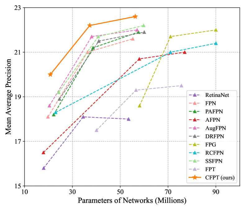
We initially compare the performance of the proposed CFPT with various state-of-the-art feature pyramid networks based on RetinaNet [1] on the VisDrone2019-DET dataset. As illustrated in Table I, our CFPT achieves the best results in RetinaNet across different backbone networks, including ResNet-18, ResNet-50, and ResNet-101, striking the optimal balance between performance and computational complexity. In addition, compared to SSFPN, which focuses on small object detection in aerial images, our CFPT achieves better performance (+0.8 AP, +0.5 AP, and +0.4 AP) with fewer parameters (-3.8 M, -3.5 M, and -3.5 M) and lower FLOPs (-55.5 G). This demonstrates the applicability of CFPT for small object detection in aerial images.
IV-D Comparison with State-of-the-Art Methods
To further verify the effectiveness of CFPT, we replace the feature pyramid network in state-of-the-art detectors with CFPT and compare their performance on the VisDrone2019-DET and TinyPerson datasets.
IV-D1 VisDrone2019-DET
We replace the feature pyramid in GFL [43] with CFPT and compare its performance with various state-of-the-art detectors. As shown in Table II, the application of our CFPT improves the performance of GFL by 0.8 AP, 0.7 AP, and 0.7 AP based on ResNet-18, ResNet-50, and ResNet-101, respectively. While there is a slight increase in the number of parameters by 0.3 M, 0.2 M, and 0.2 M. Compared with CEASC [20], our parameters increase by only 0.1 M, yet achieve significant performance gains (+0.7 AP, +0.6 AP, and +0.6 AP), proving the effectiveness of our CFPT.
IV-D2 TinyPerson
For the comparison on the TinyPerson dataset, we use the evaluation metrics defined in [3] to thoroughly assess the model’s performance. We observe that GFL [43] excels in fine-grained detection, as indicated by its superior performance on the AP-tiny75 metric, whereas FSAF [41] is more effective for coarse-grained prediction, demonstrated by its better performance on the AP-tiny25 and AP-tiny50 metrics. Therefore, we integrate CFPT into both GFL and FSAF to evaluate its adaptability to these two scenarios. As shown in Table III, CFPT delivers significant performance improvements, including a 2.4 AP-tiny gain for GFL (44.2 AP-tiny v.s 41.8 AP-tiny) and a 2.0 AP-tiny gain for FSAF (44.5 AP-tiny v.s 42.5 AP-tiny), with all performance indicators showing enhancements. Therefore, integrating CFPT effectively improves the small object detection performance of the model, demonstrating its efficacy for small object detection in aerial images.
| Method | AP-tiny(%) | AP-tiny25(%) | AP-tiny125(%) | AP-tiny225(%) | AP-tiny325(%) | AP-tiny50(%) | AP-tiny75(%) |
|---|---|---|---|---|---|---|---|
| RetinaNet | 29.9 | 59.4 | 33.1 | 61.3 | 79.1 | 27.9 | 2.4 |
| PISA | 33.2 | 56.7 | 58.9 | 59.1 | 80.8 | 37.5 | 5.4 |
| Reppoints | 33.4 | 66.6 | 45.6 | 70.8 | 78.8 | 31.7 | 2.0 |
| LibraRCNN | 35.6 | 60.9 | 57.7 | 59.1 | 82.9 | 41.2 | 4.8 |
| FasterRCNN | 36.5 | 64.2 | 56.2 | 64.7 | 84.7 | 41.0 | 4.2 |
| DynamicRCNN | 36.8 | 63.8 | 54.0 | 61.7 | 80.4 | 41.5 | 5.0 |
| PAA | 37.9 | 66.8 | 47.8 | 68.1 | 79.7 | 41.8 | 5.0 |
| CascadeRCNN | 38.8 | 66.9 | 51.0 | 67.6 | 84.5 | 44.4 | 5.2 |
| VFL | 39.0 | 68.5 | 54.6 | 73.4 | 79.7 | 43.0 | 5.4 |
| GFL | 41.8 | 70.9 | 54.5 | 75.0 | 82.2 | 48.1 | 6.6 |
| FSAF | 42.5 | 74.3 | 62.1 | 76.2 | 83.3 | 47.5 | 5.6 |
| GFL + CFPT (ours) | 44.2 | 74.6 | 62.5 | 77.8 | 83.6 | 51.0 | 7.0 |
| FSAF + CFPT (ours) | 44.5 | 76.4 | 62.3 | 79.2 | 85.4 | 51.4 | 5.8 |
IV-E Ablation Study
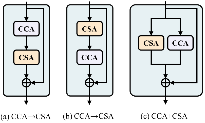
IV-E1 Order of CCA and CSA
We investigate the impact of the order in which CCA and CSA are applied on model performance. Specifically, we compare the performance of three solutions, as shown in Figure 7, including CCACSA, CSACCA, and CCACSA. As illustrate in Table IV, the CCACSA pattern achieves optimal performance with an AP of 22.2. We believe this is because the CCA provides a global receptive field along the spatial direction, enabling the CSA to utilize global contextual information to predict more accurate attention maps and obtain preferred neighboring details information. However, since CSA has a global receptive field along the channel direction, placing it first may disrupt locality and prevent CCA from accurately focusing on spatial-wise neighboring information. In addition, CCACSA will result in no interaction between CCA and CSA, making it impossible to use each other’s information for refined information aggregation.
| Method | AP(%) | AP0.5(%) | AP0.75(%) | AP-small(%) |
|---|---|---|---|---|
| CCA CSA | 22.2 | 38.0 | 22.4 | 11.9 |
| CSA CCA | 22.1 | 37.7 | 22.4 | 11.9 |
| CCA CSA | 22.0 | 37.4 | 22.2 | 11.6 |
IV-E2 Effectiveness of each proposed component
We evaluate the effectiveness of each component by progressively integrating the proposed modules into the baseline model (i.e., RetinaNet without FPN). As indicated in Table V, the integration of CCA and CSA enhances the baseline model significantly by 3.5 AP and 3.4 AP, respectively. By integrating CCA and CSA into a comprehensive CAM, the model achieves an AP gain of 3.9 AP (22.0 AP vs. 18.1 AP). The subsequent application of CCPE further enhances the performance of the model, resulting in a final AP of 22.2. It is noteworthy that integrating either CCA or CSA achieves superior performance compared to most feature pyramid networks in Table I, highlighting their potential for small object detection in aerial images.
We also report the impact of each component on the model’s computational complexity, number of parameters, and inference speed in Table V. When using only a single component (e.g., CCA), CFPT introduces an additional 1.4 M parameters, 7.4 G FLOPs, and 0.004 s/img of inference latency compared to the baseline model, while achieving significant performance gains (+3.5 AP). When all components are used, CFPT introduces an additional 2.8 M parameters, 14.8 G FLOPs, and 0.01 s/img of inference latency, while achieving significant performance gains (+4.1 AP). Therefore, CFPT can achieve a better balance between performance and computational complexity.
| CCA | CSA | CCPE | AP(%) | AP0.5(%) | AP0.75(%) | AP-small(%) | Params(M) | FLOPs(G) | Inference Speed(s/img) |
|---|---|---|---|---|---|---|---|---|---|
| Baseline [1] | 18.1 | 31.1 | 18.3 | 8.8 | 34.5 | 203.7 | 0.039 | ||
| 21.6 | 36.8 | 21.9 | 11.2 | 35.9 | 211.1 | 0.043 | |||
| 21.5 | 36.8 | 21.7 | 11.5 | 35.9 | 211.1 | 0.044 | |||
| 22.0 | 37.6 | 22.2 | 11.8 | 37.2 | 218.5 | 0.049 | |||
| 22.2(+4.1) | 38.0 | 22.4 | 11.9 | 37.3 | 218.5 | 0.049 | |||
IV-E3 Number of CAMs
We assess the impact of the number of CAMs on model performance. As shown in Table VI, increasing the number of CAMs consistently enhances the model’s performance. With three CAMs, the model achieves an AP of 22.5, marking a gain of 4.4 AP compared to the baseline (22.5 AP v.s 18.1 AP). To better balance computational complexity and performance, we set the stacking number of CAM to 1 in all other experiments, even though more CAMs would bring more benefits.
| Method | AP(%) | AP0.5(%) | AP0.75(%) | AP-small(%) | Params(M) |
|---|---|---|---|---|---|
| 1 | 22.2 | 38.0 | 22.4 | 11.9 | 37.3 |
| 2 | 22.3 | 38.0 | 22.7 | 12.2 | 40.0 |
| 3 | 22.5 | 38.5 | 22.8 | 12.3 | 42.8 |
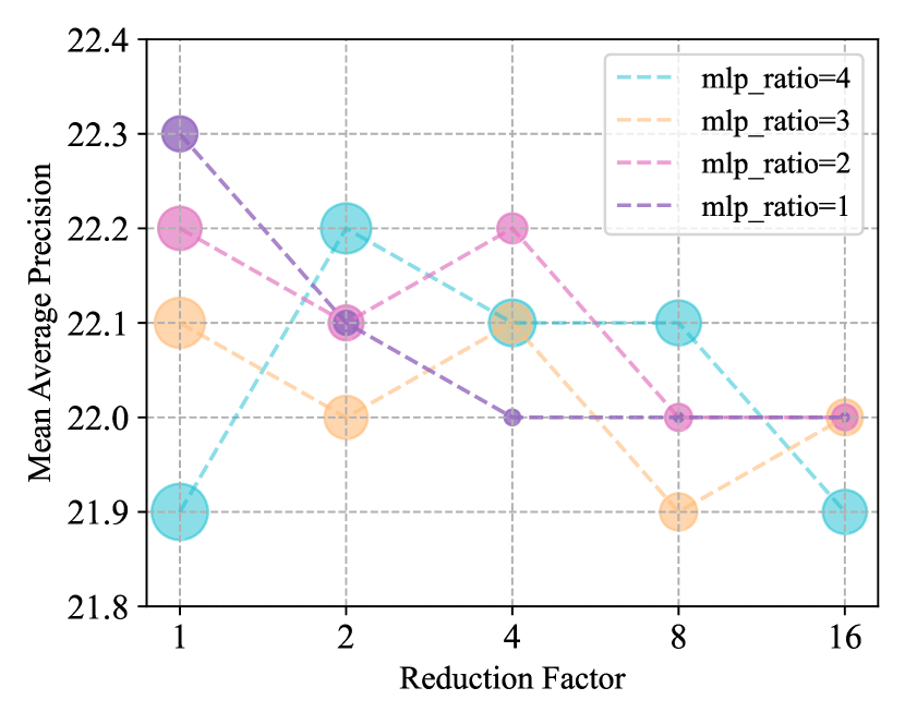
IV-E4 Channel Size reduction factor and MLP ratio
We investigate the effects of various channel size reduction factors (i.e., the compression factor of feature map channels for attention interactions) and MLP ratios (i.e., the expansion factor for channel size in FFNs), aiming to identify the optimal combination that balances computational complexity and model performance. As shown in Fig. 9, the model achieves the optimal balance between computational complexity and performance when the channel size reduction factor is set to 4 and the MLP ratio is set to 2. Therefore, for all experiments conducted on the VisDrone2019-DET and TinyPerson datasets, we consistently use this combination scheme.
IV-F Qualitative Analysis
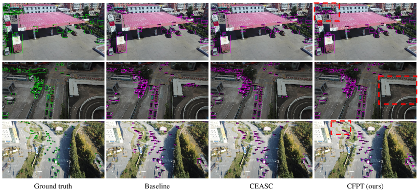
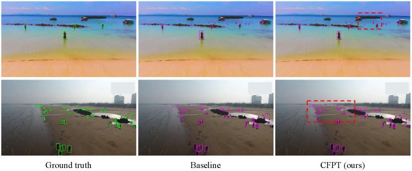
We conduct the qualitative analysis of CFPT by visualizing the detection results on the VisDrone2019-DET and TinyPerson datasets, with the confidence threshold for all visualizations set to 0.3. As shown in Fig. 8, we apply CFPT to GFL and compare it qualitatively with the baseline model (i.e., GFL) and CEASC on VisDrone2019-DET dataset. The application of CFPT effectively reduces the model’s missed detection rate (first and third rows) and false detection rate (second row), thereby improving its overall performance. In addition, the third row of Fig. 8 demonstrates CFPT’s effectiveness in detecting small objects. As shown in Fig. 10, the detection results on the TinyPerson dataset further validate the above explanations, demonstrating that CFPT effectively reduces the missed detection and false detection rates while enhancing the model’s ability to detect small objects.
V Conclusion
In this paper, we introduce CFPT, a novel upsampler-free feature pyramid network designed for small object detection in aerial images. CFPT can explicitly focus more on shallow feature maps and forgo the static kernel-based interaction schemes to mitigate the impact of scale differences on model performance, making it particularly well-suited for object detection in aerial images. Specifically, CFPT comprises two meticulously designed attention blocks with linear computational complexity, namely CCA and CSA. The two modules capture contextual information from different perspectives, and their integration provides the model with essential global contextual modeling capabilities crucial for detecting small objects. Furthermore, to enhance positional awareness during cross-layer interaction, we propose a new positional encoding method called CCPE. Extensive experiments on two challenging aerial datasets demonstrate that CFPT outperforms state-of-the-art feature pyramid networks while also reducing computational costs. In future work, we plan to explore deformable cross-layer interaction solutions and investigate more efficient implementation strategies.
References
- [1] T.-Y. Lin, P. Goyal, R. Girshick, K. He, and P. Dollár, “Focal loss for dense object detection,” in Proc. IEEE Int. Conf. Comp. Vis., 2017, pp. 2980–2988.
- [2] D. Du, P. Zhu, L. Wen, X. Bian, H. Lin, Q. Hu, T. Peng, J. Zheng, X. Wang, Y. Zhang et al., “Visdrone-det2019: The vision meets drone object detection in image challenge results,” in Proc. IEEE Int. Conf. Comp. Vis. Workshops., 2019, pp. 0–0.
- [3] X. Yu, Y. Gong, N. Jiang, Q. Ye, and Z. Han, “Scale match for tiny person detection,” in Proc. Winter Conf. Applications of Comp. Vis., 2020, pp. 1257–1265.
- [4] S. Deng, S. Li, K. Xie, W. Song, X. Liao, A. Hao, and H. Qin, “A global-local self-adaptive network for drone-view object detection,” IEEE Trans. Image Process., vol. 30, pp. 1556–1569, 2020.
- [5] J. Leng, M. Mo, Y. Zhou, C. Gao, W. Li, and X. Gao, “Pareto refocusing for drone-view object detection,” IEEE Trans. Circuits Syst. Video Technol., vol. 33, no. 3, pp. 1320–1334, 2022.
- [6] Y. Huang, J. Chen, and D. Huang, “Ufpmp-det: Toward accurate and efficient object detection on drone imagery,” in Proc. Conf. AAAI, vol. 36, no. 1, 2022, pp. 1026–1033.
- [7] T.-Y. Lin, P. Dollár, R. Girshick, K. He, B. Hariharan, and S. Belongie, “Feature pyramid networks for object detection,” in Proc. IEEE Conf. Comp. Vis. Patt. Recogn., 2017, pp. 2117–2125.
- [8] K. Chen, Y. Cao, C. C. Loy, D. Lin, and C. Feichtenhofer, “Feature pyramid grids,” arXiv preprint arXiv:2004.03580, 2020.
- [9] M. Tan, R. Pang, and Q. V. Le, “Efficientdet: Scalable and efficient object detection,” in Proc. IEEE Conf. Comp. Vis. Patt. Recogn., 2020, pp. 10 781–10 790.
- [10] D. Zhang, H. Zhang, J. Tang, M. Wang, X. Hua, and Q. Sun, “Feature pyramid transformer,” in Proc. Eur. Conf. Comp. Vis. Springer, 2020, pp. 323–339.
- [11] G. Yang, J. Lei, Z. Zhu, S. Cheng, Z. Feng, and R. Liang, “Afpn: Asymptotic feature pyramid network for object detection,” in IEEE Trans. Syst., Man, Cybern. IEEE, 2023, pp. 2184–2189.
- [12] S. Liu, L. Qi, H. Qin, J. Shi, and J. Jia, “Path aggregation network for instance segmentation,” in Proc. IEEE Conf. Comp. Vis. Patt. Recogn., 2018, pp. 8759–8768.
- [13] D. Shi, “Transnext: Robust foveal visual perception for vision transformers,” in Proc. IEEE Conf. Comp. Vis. Patt. Recogn., 2024, pp. 17 773–17 783.
- [14] J. Redmon, S. Divvala, R. Girshick, and A. Farhadi, “You only look once: Unified, real-time object detection,” in Proc. IEEE Conf. Comp. Vis. Patt. Recogn., 2016, pp. 779–788.
- [15] S. Ren, K. He, R. Girshick, and J. Sun, “Faster r-cnn: Towards real-time object detection with region proposal networks,” Advances in Neural Inf. Process. Syst., vol. 28, 2015.
- [16] A. Wang, H. Chen, L. Liu, K. Chen, Z. Lin, J. Han, and G. Ding, “Yolov10: Real-time end-to-end object detection,” arXiv preprint arXiv:2405.14458, 2024.
- [17] F. Yang, H. Fan, P. Chu, E. Blasch, and H. Ling, “Clustered object detection in aerial images,” in Proc. IEEE Int. Conf. Comp. Vis., 2019, pp. 8311–8320.
- [18] C. Li, T. Yang, S. Zhu, C. Chen, and S. Guan, “Density map guided object detection in aerial images,” in Proc. IEEE Conf. Comp. Vis. Patt. Recogn. Workshops., 2020, pp. 190–191.
- [19] Y. Wang, Y. Yang, and X. Zhao, “Object detection using clustering algorithm adaptive searching regions in aerial images,” in Proc. Eur. Conf. Comp. Vis. Springer, 2020, pp. 651–664.
- [20] B. Du, Y. Huang, J. Chen, and D. Huang, “Adaptive sparse convolutional networks with global context enhancement for faster object detection on drone images,” in Proc. IEEE Conf. Comp. Vis. Patt. Recogn., 2023, pp. 13 435–13 444.
- [21] L. Chen, C. Liu, W. Li, Q. Xu, and H. Deng, “Dtssnet: Dynamic training sample selection network for uav object detection,” IEEE Trans. Geo. Remote Sens., 2024.
- [22] J. Pang, K. Chen, J. Shi, H. Feng, W. Ouyang, and D. Lin, “Libra r-cnn: Towards balanced learning for object detection,” in Proc. IEEE Conf. Comp. Vis. Patt. Recogn., 2019, pp. 821–830.
- [23] C. Guo, B. Fan, Q. Zhang, S. Xiang, and C. Pan, “Augfpn: Improving multi-scale feature learning for object detection,” in Proc. IEEE Conf. Comp. Vis. Patt. Recogn., 2020, pp. 12 595–12 604.
- [24] A. Vaswani, N. Shazeer, N. Parmar, J. Uszkoreit, L. Jones, A. N. Gomez, Ł. Kaiser, and I. Polosukhin, “Attention is all you need,” Advances in Neural Inf. Process. Syst., vol. 30, 2017.
- [25] A. Dosovitskiy, L. Beyer, A. Kolesnikov, D. Weissenborn, X. Zhai, T. Unterthiner, M. Dehghani, M. Minderer, G. Heigold, S. Gelly et al., “An image is worth 16x16 words: Transformers for image recognition at scale,” arXiv preprint arXiv:2010.11929, 2020.
- [26] L. Lin, H. Fan, Z. Zhang, Y. Xu, and H. Ling, “Swintrack: A simple and strong baseline for transformer tracking,” Advances in Neural Inf. Process. Syst., vol. 35, pp. 16 743–16 754, 2022.
- [27] Y. Peng, Y. Zhang, B. Tu, Q. Li, and W. Li, “Spatial–spectral transformer with cross-attention for hyperspectral image classification,” IEEE Trans. Geo. Remote Sens., vol. 60, pp. 1–15, 2022.
- [28] T. Xiao, Y. Liu, Y. Huang, M. Li, and G. Yang, “Enhancing multiscale representations with transformer for remote sensing image semantic segmentation,” IEEE Trans. Geo. Remote Sens., vol. 61, pp. 1–16, 2023.
- [29] Z. Liu, Y. Lin, Y. Cao, H. Hu, Y. Wei, Z. Zhang, S. Lin, and B. Guo, “Swin transformer: Hierarchical vision transformer using shifted windows,” in Proc. IEEE Int. Conf. Comp. Vis., 2021, pp. 10 012–10 022.
- [30] P. Ramachandran, N. Parmar, A. Vaswani, I. Bello, A. Levskaya, and J. Shlens, “Stand-alone self-attention in vision models,” Advances in Neural Inf. Process. Syst., vol. 32, 2019.
- [31] H. Zhao, J. Jia, and V. Koltun, “Exploring self-attention for image recognition,” in Proc. IEEE Conf. Comp. Vis. Patt. Recogn., 2020, pp. 10 076–10 085.
- [32] X. Pan, T. Ye, Z. Xia, S. Song, and G. Huang, “Slide-transformer: Hierarchical vision transformer with local self-attention,” in Proc. IEEE Conf. Comp. Vis. Patt. Recogn., 2023, pp. 2082–2091.
- [33] J. Ho, N. Kalchbrenner, D. Weissenborn, and T. Salimans, “Axial attention in multidimensional transformers,” arXiv preprint arXiv:1912.12180, 2019.
- [34] K. He, X. Zhang, S. Ren, and J. Sun, “Deep residual learning for image recognition,” in Proc. IEEE Conf. Comp. Vis. Patt. Recogn., 2016, pp. 770–778.
- [35] J. Ma and B. Chen, “Dual refinement feature pyramid networks for object detection,” arXiv preprint arXiv:2012.01733, 2020.
- [36] Z. Zong, Q. Cao, and B. Leng, “Rcnet: Reverse feature pyramid and cross-scale shift network for object detection,” in Proc. ACM Int. Conf. Multimedia, 2021, pp. 5637–5645.
- [37] M. Hong, S. Li, Y. Yang, F. Zhu, Q. Zhao, and L. Lu, “Sspnet: Scale selection pyramid network for tiny person detection from uav images,” IEEE Geo. Remote Sens. Letters., vol. 19, pp. 1–5, 2021.
- [38] Z. Cai and N. Vasconcelos, “Cascade r-cnn: Delving into high quality object detection,” in Proc. IEEE Conf. Comp. Vis. Patt. Recogn., 2018, pp. 6154–6162.
- [39] Y. Cao, K. Chen, C. C. Loy, and D. Lin, “Prime sample attention in object detection,” in Proc. IEEE Conf. Comp. Vis. Patt. Recogn., 2020, pp. 11 583–11 591.
- [40] H. Zhang, H. Chang, B. Ma, N. Wang, and X. Chen, “Dynamic r-cnn: Towards high quality object detection via dynamic training,” in Proc. Eur. Conf. Comp. Vis. Springer, 2020, pp. 260–275.
- [41] C. Zhu, Y. He, and M. Savvides, “Feature selective anchor-free module for single-shot object detection,” in Proc. IEEE Conf. Comp. Vis. Patt. Recogn., 2019, pp. 840–849.
- [42] S. Zhang, C. Chi, Y. Yao, Z. Lei, and S. Z. Li, “Bridging the gap between anchor-based and anchor-free detection via adaptive training sample selection,” in Proc. IEEE Conf. Comp. Vis. Patt. Recogn., 2020, pp. 9759–9768.
- [43] X. Li, W. Wang, L. Wu, S. Chen, X. Hu, J. Li, J. Tang, and J. Yang, “Generalized focal loss: Learning qualified and distributed bounding boxes for dense object detection,” Advances in Neural Inf. Process. Syst., vol. 33, pp. 21 002–21 012, 2020.
- [44] C. Feng, Y. Zhong, Y. Gao, M. R. Scott, and W. Huang, “Tood: Task-aligned one-stage object detection,” in Proc. IEEE Int. Conf. Comp. Vis. IEEE Computer Society, 2021, pp. 3490–3499.
- [45] H. Zhang, Y. Wang, F. Dayoub, and N. Sunderhauf, “Varifocalnet: An iou-aware dense object detector,” in Proc. IEEE Conf. Comp. Vis. Patt. Recogn., 2021, pp. 8514–8523.
- [46] X. Li, W. Wang, X. Hu, J. Li, J. Tang, and J. Yang, “Generalized focal loss v2: Learning reliable localization quality estimation for dense object detection,” in Proc. IEEE Conf. Comp. Vis. Patt. Recogn., 2021, pp. 11 632–11 641.
- [47] C. Yang, Z. Huang, and N. Wang, “Querydet: Cascaded sparse query for accelerating high-resolution small object detection,” in Proc. IEEE Conf. Comp. Vis. Patt. Recogn., 2022, pp. 13 668–13 677.
- [48] A. Paszke, S. Gross, F. Massa, A. Lerer, J. Bradbury, G. Chanan, T. Killeen, Z. Lin, N. Gimelshein, L. Antiga et al., “Pytorch: An imperative style, high-performance deep learning library,” Advances in Neural Inf. Process. Syst., vol. 32, 2019.
- [49] K. Chen, J. Wang, J. Pang, Y. Cao, Y. Xiong, X. Li, S. Sun, W. Feng, Z. Liu, J. Xu et al., “Mmdetection: Open mmlab detection toolbox and benchmark,” arXiv preprint arXiv:1906.07155, 2019.