Creating stars orbiting in AdS

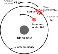
Fig.1 shows a schematic image of our setup. We consider the pure global AdS and Schwarzschild-AdS₄ (Sch-AdS₄) spacetime with a spherical horizon as the background spacetimes. These correspond to the ($2+1$)-dimensional quantum field theory (QFT) on $S^{2}$. We deal with the bulk scalar field as the probe, which corresponds to a scalar operator $\mathcal{O}$ in the dual QFT. We regard the operator $\mathcal{O}$ as the source of the bulk field. The source is localized in $S^{2}$, and its packet rotates with angular velocity $\Omega$. It also has frequency $\omega$ and wavenumber $m$. We demonstrate that by tuning the parameters $(\omega,m,\Omega)$, a bulk star is created.

Previous studies have proposed that gravitational lensing can be used to test the existence of a given QFT [10, 11, 12, 13]. The Einstein ring formed by gravitational lensing provides information about the photon sphere of the null geodesic in dual geometry. In this letter, we propose another method to probe dual geometry using the timelike geodesic. In Refs.[14, 15], dual operators corresponding to localised states in the AdS bulk have been investigated. Our work provides an explicit source function for creating similar states through a time evolution.

 
Eikonal approximation for massive scalar field— We consider the Sch-AdS₄ with the spherical horizon as

where $f(r)=1+r^{2}-r_{h}(1+r_{h}^{2})/r$ in units of the AdS radius. For $r_{h}=0$, this spacetime describes the pure global AdS. Let us consider the circular orbit of the massive particle in this spacetime. The specific energy and angular momentum of the particle are given by $\epsilon\equiv-u_{t}$ and $j\equiv u_{\phi}$, where $u^{\mu}$ is the 4-velocity. The angular velocity of revolution is $\Omega\equiv d\phi/dt=u^{\phi}/u^{t}$. For a circular orbit with radius $r=R$, the parameters of the timelike geodesic ($\epsilon$, $j$, $\Omega$) are given by the one-parameter family of $R$ (for fixed $r_{h}$) as

We will consider the creation of the massive particle (or star) as the coherent excitation of the bulk field.

We deal with the massive scalar field in a fixed background whose Lagrangian is given by:

The scalar field obeys the Klein-Gordon equation $\square\Phi=\mu^{2}\Phi$. Using the Eikonal approximation, we can obtain the timelike geodesic equation from the Klein-Gordon equation. We assume that the typical frequency $\omega$ and mass $\mu$ of the scalar field are sufficiently large, and that they are of the same order, $\omega\sim\mu\gg 1$. Substituting $\Phi(x^{\mu})=a(x^{\mu})e^{iS(x^{\mu})}$ into the Klein-Gordon equation and assuming $\partial_{\mu}S\sim\mathcal{O}(\omega)$, we obtain

as the leading-order equation for $\omega$. Introducing the 4-velocity $u_{\mu}=\partial_{\mu}S/\mu$, we have $u_{\mu}u^{\mu}=-1$. Differentiating this equation, we also obtain the geodesic equation for a massive particle as $0=\nabla_{\rho}(g^{\mu\nu}\partial_{\mu}S\partial_{\nu}S)/\mu^{2}=2u^{\mu}\nabla_{\mu}u_{\rho}$. Thus, the relationship between the parameters of the timelike geodesic and the massive scalar field is

Analysis of the Eikonal approximation indicates that massive particles should also be expressed as the localized configuration of the massive scalar field. Our main task is to determine the appropriate boundary condition for the scalar field at the AdS boundary and create a particle (or star) orbiting in AdS, as shown in Fig.1.

 
Massive scalar field in asymptotically AdS spacetimes— Near the AdS boundary $r=\infty$, the scalar field behaves as

where $\Delta_{\pm}=3/2\pm\nu$ and $\nu=\sqrt{9/4+\mu^{2}}$. We refer to $\mathcal{J}(t,\theta,\phi)$ and $\langle\mathcal{O}(t,\theta,\phi)\rangle$ as the “source” and “response”, respectively.

Caution is needed when considering the “source” for the massive scalar field. For $\mu^{2}>0$, the corresponding operator $\mathcal{O}$ has a conformal weight $\Delta_{+}>3$, and applying the source to such an operator corresponds to an irrelevant deformation of the dual QFT. From a gravitational point of view, if a non-asymptotically mode is present, the energy-momentum tensor of the scalar field diverges near the AdS boundary and the probe approximation is no longer valid  [16]. One way to avoid this problem is to introduce an explicit cutoff at the finite radius of asymptotically AdS spacetime. The AdS with a finite radial cutoff is considered the gravitational dual of the $T\bar{T}$-deformed theory [17]. The other way is to introduce a renormalization group flow to a UV fixed point where $\mathcal{O}$ is relevant. One of the simplest examples is the addition of another scalar field $\psi$, which controls the mass for $\Phi$:

where $\lambda(\psi)$ is now a function of the dynamic scalar field $\psi$. Because the mass square of $\psi$ is $-2$, $\psi$ behaves as $\psi\sim 1/r,1/r^{2}$ near the AdS boundary, and both modes are normalizable. When $\Phi=0$, we can obtain a static and spherically symmetric profile $\psi=\psi(r)$ by imposing only the regularity at the horizon or centre of the global AdS. (Then, both the $1/r$ and $1/r^{2}$ modes are present at the AdS boundary in general.) By carefully choosing the mass function $\lambda(\psi)$, for example, $\lambda(\psi)=\mu\tanh(\psi)$, the effective mass for $\Phi$ can be almost constant, except for the region near the AdS boundary. Considering the infinitesimal perturbation of $\Phi$, we have a scalar field whose mass vanishes near the AdS boundary and whose energy-momentum tensor is still finite. (The backreaction to $\psi$ is second-order in $\Phi$ and negligible.) Let us take the cutoff $r=\Lambda$ so that

is satisfied. We consider only the region $r\lesssim\Lambda$, where the theory is described by Eq.(3). Subsequently, the “source” in Eq.(6) can be regarded as $\mathcal{J}\simeq r^{\Delta_{-}}\Phi|_{r=\Lambda}$. Although this $\mathcal{J}$ is different from the “real” source defined in UV-complete theory (7), $\mathcal{J}_{\textrm{UV}}=\Phi|_{r=\infty}$, we assume that they are qualitatively similar because $\Phi(r=\Lambda)$ and $\Phi(r=\infty)$ are only related to the $r$ evolution of the equation of motion derived from Eq.(7). In this letter, we refer to $\mathcal{J}$ as the source.

 
Massive scalar field localized in bounded orbit.— We adopt the following form of the source function:

This function is localized in $S^{2}$ at $\theta=\pi/2$ and $\phi=\Omega t$, with widths $\sigma_{\theta}$ and $\sigma_{\phi}$, respectively. (We take the domain of the coordinate $\phi$ as $-\pi<\phi-\Omega t\leq\pi$.) The centre of the localized source rotates on the equator with angular velocity $\Omega$. This has a wavenumber $m$ along the $\phi$-direction and oscillates over time with frequency $\omega$. (See Fig.1 for the schematic picture of the source.) The source is also localized in time at $t=T$ with width $\sigma_{t}$. We take a large $\sigma_{t}$ such that the modes with frequency $\sim\omega$ are sufficiently excited. We take $T<0$ and $\sigma_{t}\ll|T|$ such that the application of the source has already been terminated at $t=0$. $J_{0}$ is the amplitude of the source; however, it is not important in our analysis because of the linearity of the scalar field.

There are some requirements for the parameters in Eq.(9) to realise a localized star in the bulk. The scalar field induced by the source (9) typically has a frequency $\omega$ and wavenumber $m$. In addition, its angular size is determined by $\sigma_{\theta}$ and $\sigma_{\phi}$. Conversely, in momentum space, the scalar field is distributed with a width $\sim 1/\sigma_{\phi},1/\sigma_{\theta}$. Therefore, the condition that the scalar field is localized in both the real and momentum spaces is given by:

It is also necessary that $\omega$ and $\mu$ be sufficiently large compared with the curvature scale of the bulk geometry, so that the Eikonal approximation is valid.

Eq.(9) is regarded as the boundary condition of the scalar field near the AdS boundary. We now explain how this boundary condition is imposed and the equation of motion for the scalar field is solved. If we decompose $\Phi$ as $\Phi=r^{-1}\sum_{\omega^{\prime}m^{\prime}l^{\prime}}e^{-i\omega^{\prime}t}\Psi_{\omega^{\prime}l^{\prime}m^{\prime}}(x)Y_{l^{\prime}m^{\prime}}(\theta,\phi)$, where $Y_{l^{\prime}m^{\prime}}$ is the spherical harmonics, then $\Psi_{\omega l^{\prime}m^{\prime}}(x)$ obeys the equation in the Schrödinger form:

where $x=\int dr/f(r)$ is the tortoise coordinate. We can also decompose the source (9) as

The coefficient $J_{\omega^{\prime}l^{\prime}m^{\prime}}$ provides the boundary condition for $\Psi_{\omega^{\prime}l^{\prime}m^{\prime}}(x)$ at the AdS boundary: $\Psi_{\omega^{\prime}l^{\prime}m^{\prime}}(x)\to J_{\omega^{\prime}l^{\prime}m^{\prime}}r^{-\Delta_{-}+1}$. For $r_{h}>0$, we impose the ingoing wave boundary condition at horizon $\Psi_{\omega^{\prime}l^{\prime}m^{\prime}}(x)\sim e^{-i\omega^{\prime}x}$. For $r_{h}=0$, we impose regularity at the centre of the AdS, $\Psi_{\omega^{\prime}l^{\prime}m^{\prime}}(x)\sim r^{l^{\prime}}$. Under these boundary conditions, Eq.(11), and superposing the numerically obtained solutions, we obtain the scalar field in real space $\Phi(t,r,\theta,\phi)$. (See the supplementary material for details).

For source (9), the typical frequency and wavenumber of the bulk scalar field are given by $\omega$ and $m$, respectively. From Eq.(5), the specific energy and angular momentum of the created star are given by

We can expect the angular velocity of the revolution of the star to be determined by $\Omega$ in Eq.(9). This is verified by our numerical results. The rest mass is the energy measured by the observer accompanying the star: $\sim\int d\Sigma T_{\mu\nu}u^{\mu}u^{\nu}$, where $T_{\mu\nu}$ is the energy-momentum tensor of the scalar field and $\int d\Sigma$ denotes the integral on the $t=$const surface. This is proportional to $|J_{0}|^{2}$ with other parameters fixed. The relationships between the parameters of the created star and those of the external source are summarized in Table 1. The scalar field is localized at the local minimum of the effective potential $V(x)$. The radial size is determined by its curvature $\sigma_{x}=(V_{,xx}|_{\textrm{local min}})^{-1/2}$.

Note that Table 1 does not mean that a star is created for any value of $\omega$, $m$, and $\Omega$. As in Eq.(2), $\epsilon$, $j$, and $\Omega$ are given by the one-parameter family of the radius of circular orbit $R$. Hence, if we want to create a star at $r=R$, we need to tune $\omega$, $m$, and $\Omega$ to the values obtained by these equations and Table 1.

 
Results.—

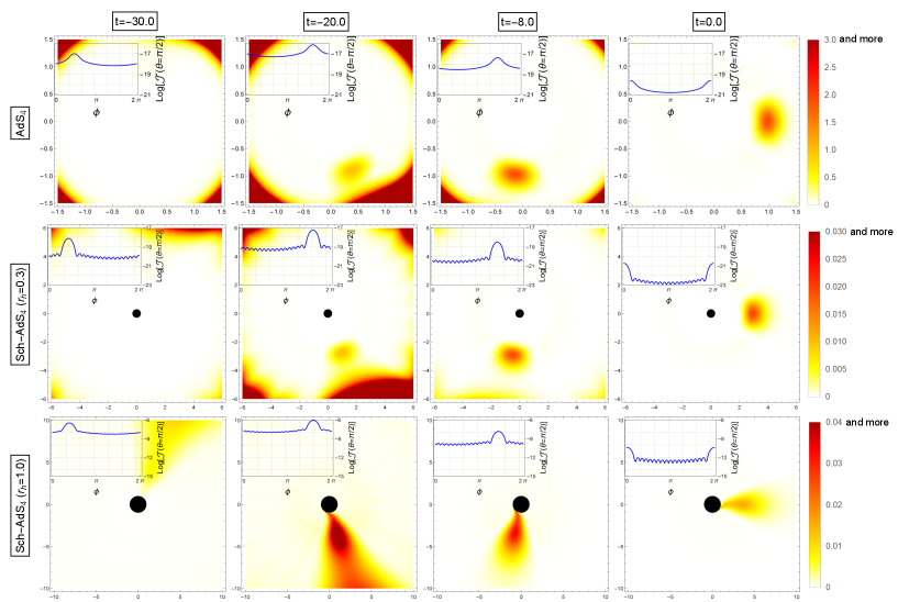
In Fig. 2, we depict the time evolution of the scalar field orbiting in the equatorial plane $\theta=\pi/2$. The parameters used in our numerical calculation are summarized in Table 2.

In addition, we set $\sigma_{\theta}=\sigma_{\phi}=0.2,T=-20,\sigma_{t}=5$. The black disks are the event horizons, and each embedded figure on the top left shows the source (9) at $\theta=\pi/2$ with respect to $\phi$. The scalar field accumulates at the local minimum of the potential (12) and forms a localized wave packet revolving anticlockwise. Using Table 1, we can estimate the specific energy $\omega/\mu$ and angular momentum $m/\mu$ of the corresponding timelike geodesic. From Eq.(5), the radii of revolution are $R\simeq 1.015,3.07,5.02$ for $r_{h}=0,0.3,1$, respectively. This was consistent with the results shown in Fig. 2 and indicates that the motion of the created star obeys the timelike geodesic equation.

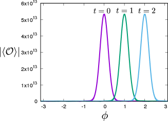
Generally, in Sch-AdS₄ spacetime, the amplitude of the scalar field decays in time because of tunnelling towards the horizon. The decay rate is characterised by the imaginary part of the quasi-normal mode frequency $\omega_{\textrm{qnm}}$. For $r_{h}=0.3$, the potential barrier is high and the decay rate is extremely suppressed. Conversely, for $r_{h}=1.0$, we have $\omega_{\textrm{qnm}}\simeq 215-0.0932i$ for $l^{\prime}=210$, and the time scale of the decay is $\tau_{\text{decay}}=10.7$. This is why the scalar field decays at a later time in the bottom line of Fig. 2]. Although we employed modest values for $\omega,m$ and $\mu$ because of the limitations of computational power, in principle, we can realise a long-lived localized scalar field by using larger values for $\omega,m$ and $\mu$ for fixed $\omega/\mu$ and $m/\mu$. Thus, a higher potential barrier is realized, and we have a small decay rate. Once we obtain the star orbiting in an asymptotically AdS spacetime, we can compute the response function from Eq.(6). In Fig. 3, we depict the response of $\theta=\pi/2$ for $r_{h}=0.3$ after the star is created $t\gtrsim 0$. The response circulates on the equator, following the orbiting scalar field. This indicates that the angular position of the star can be observed using the response function.

 
Discussion.– We demonstrated that a star orbiting in the asymptotically AdS spacetime can be created by applying the appropriate source (9) in the dual QFT. The parameters in the source should be tuned to create the localized star. If the dual geometry is known, we can determine the parameters by studying the timelike geodesic, as in Eq.(5). However, for a real material, in general, we do not know the dual geometry explicitly. Thus, in a real experiment, we must tune the parameters $\omega$, $m$, and $\Omega$ by trial and error. The creation of a star in the bulk is verified by the response function, as shown in Fig.3. Once we can create a star in the bulk, we obtain the relationship between $\epsilon$, $m$, and $\Omega$: $j=j(\epsilon)$ and $\Omega=\Omega(\epsilon)$. This provides information regarding the geometry of the AdS bulk.

In this letter, only a circular orbit was considered: the scalar field was radially localised at the local minimum of the potential (12). The non-circular orbit is the coherent excitation around the local minimum. Such a bulk coherent state can be realized by varying $J_{0}$ in time in the source (9). Observing the star in the non-circular orbit through the response function, we can obtain information about a wider region of the bulk geometry.