Cramér-Rao bound and quantum parameter estimation with non-Hermitian systems
Abstract
The quantum Fisher information constrains the achievable precision in parameter estimation via the quantum Cramér-Rao bound, which has attracted much attention in Hermitian systems since the 60s of the last century. However, less attention has been paid to non-Hermitian systems. In this Letter, working with different logarithmic operators, we derive two previously unknown expressions for quantum Fisher information, and two Cramér-Rao bounds lower than the well-known one are found for non-Hermitian systems. These lower bounds are due to the merit of non-Hermitian observable and it can be understood as a result of extended regimes of optimization. Two experimentally feasible examples are presented to illustrate the theory, saturation of these bounds and estimation precisions beyond the Heisenberg limit are predicted and discussed. A setup to measure non-Hermitian observable is also proposed.
Introduction.—Quantum parameter estimation helstrom67 ; helstrom76 ; holevo82 ; degen17 ; pezze18 aims at measuring the value of a continuous parameter encoded in the state of a quantum system. It gives better precision than the same measurement performed in a classical framework and plays a crucial role in the advancement of physics. The estimation process generally consists of two steps. In the first step, the state is prepared and measured. A simple way to prepare the state is to evolve a reference initial state under a signal Hamiltonian that encodes the parameter , In the second step, the estimation of is obtained by data processing the measurement outcomes, aiming at the smallest uncertainty given finite resources such as time and number of particles. The uncertainty is bounded by the Cramér-Rao bound (CRB), which expresses a lower limit on the variance of unbiased estimations, stating that the variance of any such estimation is at least as high as the inverse of the Fisher information fisher25 ; matson06 .
The quantum Cramér-Rao bound works in general with Hermitian quantum systems frieden90 ; braunstein94 ; liu20 in order to meet the requirement of quantum mechanics. However, recent studies found that non-Hermitian systems with unbroken PT symmetries also possess a real spectrum bender98 . In fact, non-Hermiticity is ubiquitous in the quantum world bender07 ; guo09 , including systems with gain and/or loss konotop16m ; feng17 ; ganainy19 ; miri19 ; ozdemir19 , many-body localization and dynamical stability of non-Hermitian systems hamazaki19 , as well as sensors designed with non-Hermitian systems berry04 ; heiss12 .
These facts give rise to a question that in non-Hermitian quantum systems moiseyev11 what is the Cramér-Rao bound? This question was answered about 5 decades ago by Yuen and Lax in Ref. yuen73 , where the authors proposed an idea to estimate a complex parameter by measuring a non-Hermitian observable. Unfortunately, this theory was connected the complex parameter with the estimator by assuming that the average of the estimator is exactly the estimate of the parameter. This assumption would lead to a flaw that the error propagation function is unity, resulting in a less regime of non-Hermitian observables for optimization and experiments. Consider that the study of non-Hermitian system and their unique properties have attracted fast growing interest in the last two decades, revisiting the quantum Cramér bound and its consequent estimation theory with current technologies is highly desired for non-Hermitian systems. We should address that there are estimation protocols (or sensors) based on non-Hermitian system recently wiersig14 ; liu16 ; chen17 ; hodaei17 ; djorwe19 ; mao20 , but all analyses so far are based on either the Fisher information resulting from the Hermitian quantum Cramér-Rao bound, or the properties of the exceptional points.
In this Letter, we first develop an uncertainty relation for non-Hermitian operators, then we derive two previously unknown expressions for quantum Fisher information with different logarithmic derivatives. Two quantum Cramér-Rao bounds for non-Hermitian systems are defined. We found that the Fisher information is significantly increased due to the use of non-Hermitian operators, in particular for systems in mixed states. This is in contrary to the results of Fisher information with Hermitian symmetric logarithmic derivatives. Saturation of the two bounds is analyzed and the optimal measurement to attain the bounds is derived. We elucidate the feature of non-Hermitian quantum Fisher information with GHZ states of trapped ions pezze18 ; leibried05 and the phase estimation setup with Mach-Zehnder interferometer. Comparison with the situation of non-Hermitian signal Hamiltonian is also presented and discussed.
Non-Hermitian uncertainty relation and Quantum Cramér bound.— Higher estimation precision demands more resources. The trade-off between the precision and the resources required is determined by the uncertainty principle, which constrains to what extent complementary variables maintain their averaged values and leads to the Heisenberg limit caves81 ; chin12 ; jarzyna15 ; giovannetti11 ; luis17 ; bai19 in quantum parameter estimation. One might wonder whether this is the case and how the uncertainty relation changes in non-Hermitian quantum mechanics moiseyev11 .
To explore the possible change of the uncertainty relation and introduce the variance for non-Hermitian systems, we introduce two operators and , which are linear but not necessarily Hermitian. Defining , and with a real parameter, and being the expectation value of operator , we have Simple algebra yields supp , where was defined by Operator is a Hermitian operator regardless of and being Hermitian or not. defines an abnormal commutation for operator and , which can be applied to determine whether a time-independent operator is a constant of motion for systems governed by non-Hermitian Hamiltonian rivero20 .
We define as the variance for non-Hermitian operator , which reduces to the traditional variance when is Hermitian. This uncertainty relation as well as that we will present in the following also hold for unitary operators and bong18 ; yu19 . In non-Hermitian quantum systems, the expectation value of dynamical variable might take complex values, . The absolute value and its phase are both measurable quantities. For example, in scattering experiments the peaks in the cross sections are obtained when the projectiles have energy which is equal to the absolute value of the energy, not the real part of the energy moiseyev11 . This complex expectation of non-Hermitian operator is equal to the weak value of the positive-semidefinite part of the operator multiplied by a known complex number pati15 ; nirala19 ; sahoo20 .
A stronger uncertainty relations for non-Hermitian operators and follows from the Schwarz inequality, with and and being an arbitrary state of system,
| (1) |
This is a slightly stronger inequality for the variance of operators and , which together with error propagation supp
| (2) |
leads to a quantum Cramér-Rao bound for non-Hermitian system,
| (3) |
where is defined as non-Hermitian quantum Fisher information with helstrom73ijtp ; supp
| (4) |
where is the real parameter to be estimated based on density matrix and Hermitian operator . The slightly stronger uncertainty relation Eq.(1) reduces to the Robertson-Schrödinger uncertainty relation when both and are Hermitian and returns to the unitary uncertainty relation bong18 ; yu19 with both and being unitary. Eq.(S15) was derived with an assumption that , but there is no requirement for . This indicates that Eq.(3) holds for both Hermitian and non-Hermitian . In fact, when is Hermitian, the result reduces to the widely used quantum Fisher information (denoted by hereafter) in the literature, while non-Hermitian would lead to an enhanced precision for parameter estimations as shown below.
For non-Hermitian operator , we obtain the other quantum Cramér-Rao bound leading to non-Hermitian quantum information which has the same expression as in Eq.(3) but with instead of helstrom73ijtp ; supp ,
| (5) |
There are two fundamental differences between Hermitian and non-Hermitian system in the quantum Cramér-Rao bounds defined by and , which deserve to be outlined. Firstly, in Fisher information , the observable is Hermitian but the so-call symmetric logarithmic derivative might be not. While both and in are not Hermitian. The state that encodes the parameter is Hermitian, however the signal Hamiltonian might not be Hermitian, i.e., . Secondly, in non-Hermitian system, the Fisher information is given by with and instead of in Hermitian system. As we will show later, recovers the well-known expression of quantum Fisher information for Hermitian system while can not. Whereas the Cramér-Rao bound defined by can be saturated but that by could not supp .
Fisher information of non-Hermitian system.— One of the main quests in quantum parameter estimation is to find out the highest achievable precision with given resources and design schemes that attain that precision. In general, looking for the optimal resources and schemes is difficult since one needs to optimize over the input state that encodes the parameter, the measurement that is performed at the output, and the estimator that assigns a parameter value to a given measurement outcome. One of the popular ways to obtain useful bounds in quantum parameter estimations, without the need for cumbersome optimization, is to use the quantum Fisher information. In the following, we will give an explicit expression for the non-Hermitian quantum Fisher information and in terms of the eigenstates and eigenvalues of the encoding density matrix .
Consider a -dimensional quantum system. The state of the system is parameterized by the parameter under estimation. Without loss of generality, we assume the density matrix may not be of full rank and the spectral decomposition of the density operator is,
| (6) |
Here are required to be positive for any value of and , since is the probability of the system in state . The following normalization conditions for all and are imposed. From the definition of Fisher information, we can find that,
Noticing the derivation for the two Fisher information and is different, we discuss it in the following separately.
We start our derivation of by considering a special case that with a real parameter. This assumption together with Eq.(S15) leads to,
| (7) |
and A notation was used. Clearly, as we expected. It is worth noticing that is in principle supported by the full Hilbert space, not only that spanned by the eigenstates of the density matrix. Thus the value of for can not be established by the above equations. However, these terms play an important role in the quantum Fisher information. This problem can be solved by the use of completeness relation, , i.e., . We finally arrive at supp ,
| (8) |
where This is one of the main results of this Letter. For pure state, reduce to This is the widely used quantum fisher information in literature. For mixed states with , reduces to the Hermitian Fisher information, whereas for mixed states with ,
| (9) |
where approaches to infinity in the limit of . This is not physical, since in Eq. (7) can not be established when and . In the following discussion, we will focus on the case that are -independent, such that
The quantum information can be calculated by the same technique. Different from the case of , here , for Although both and are not Hermitian, the Fisher information is real and given by supp ,
This is the other main result of this Letter. The quantum Fisher information for pure state reduces to
| (11) |
which is times smaller than in Hermitian system for pure stats. However, this is not the case for mixed states as shown in the examples below. The saturation of these bounds and the experimental measurement of non-Hermitian operator will be discussed briefly at the end of this Letter.
Examples.— Considering the Hermitian quantum Fisher information and the non-Hermitian quantum information and are almost same for pure stats, i.e., and for pure states, we focus on the case of mixed states in the undergoing examples. To simplify the expression, we consider a type of simplest mixed states—it is constructed by only two orthogonal pure states with weight and and
We first consider the maximally entangled states (or Schrödinger cat state) as the input state, which has been created with up to ions leibried05 and ions monz11 in a linear Paul trap. The encoding operator is a spin rotation defined by with Hermitian signal Hamiltonian . The case of non-Hermitian signal Hamiltonian will be discussed at the end of examples. The states that encode the parameter to construct the mixed states are,
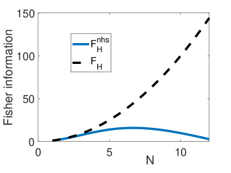
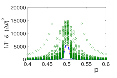
The mixed state is Notice that are -independent. The rotation generates a relative phase between states and . Straightforward calculation gives the Hermitian Fisher information and the non-Hermitian Fisher information and (setting and ) supp ,
| (12) |
The results are shown in Fig.1. We find that the non-Hermitian Fisher information are always larger than the Hermitian Fisher information, except the points
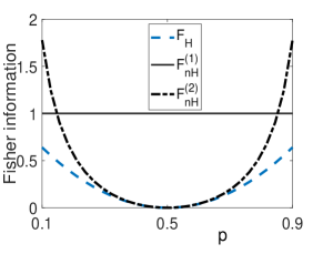
It is worth addressing that at points , the state is pure, so the Fisher information should be calculated by the formula of pure states, i.e., , and As approach to and , tends to infinity, manifesting itself as a witness of transition from mixed states to pure states. The bound defined by and can be saturated by carefully chosen measurements. For details, see Supplemental Material supp .
The second example we will show is the phase estimation interferometric schemes caves81 ; jarzyna12 , which works with coherent and squeezed vacuum states interfered at the beam-splitter of the Mach-Zehnder interferometer. Let and be the anihilation operators of the two modes. is a coherent state of mode and is a squeezed vacuum state of mode with squeezing parameter . After the input state supp has evolved through a beam splitter defined by , the estimated parameter is encoded into the state by relative phase shift operator where is the signal Hamiltonian of mode , . For the other beam splitter, see Supplemental Materials supp . We consider the following states that encode the parameter , with
| (13) |
where , and Tedious but straightforward calculations show that (set ) supp ,
| (14) |
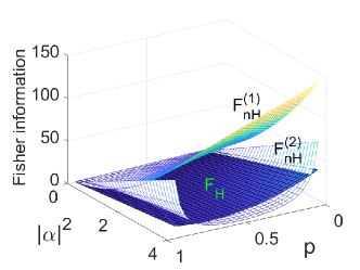
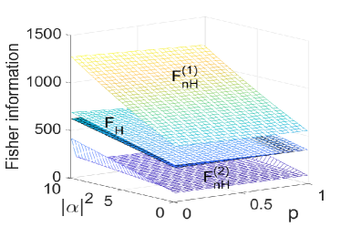
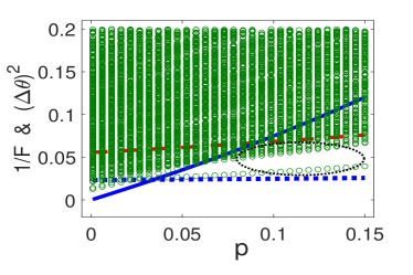
We have performed numerical calculations for the Fisher information. The results are shown in Fig. 2. We find that the two non-Hermitian quantum Fisher information favor . This can be understood as that squeezed Fock states benefit the parameter estimation more than the squeezed vacuum state. with term bounds the estimation precision beyond the Heisenberg limit of .
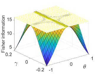
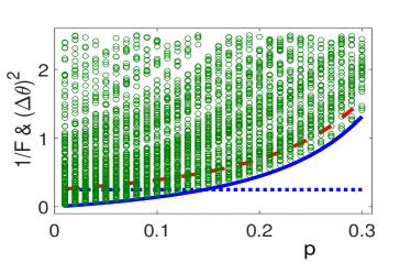
One might wonder what is the difference between the non-Hermitian Fisher information and the Hermitian Fisher information with non-Hermitian signal Hamiltonian. To answer this question, we replace the Hermitian operator by supp in the first example to calculate the Hermitian Fisher information , and the result will be denoted by . We compare with the Hermitian Fisher information with Hermitian signal Hamiltonian . In other words, the comparison is conducted between the Hermitian Fisher information with Hermitian signal and non-Hermitian signal Hamiltonian for pure states. This comparison together with what we had in the two examples would show the difference between the Hermitian and non-Hermitian Fisher information. Calculation supp finds,
| (15) |
where Numerical results are given in Fig.3. We find is smaller than for almost all and , except and very close to zero. The difference between and can be interpreted by a residual dependence of the state on the parameter under estimation apart from the statistical manifold of states. This happens, for example, when the eigenstates of the density matrix have a parameter-dependent normalization seveso17 .
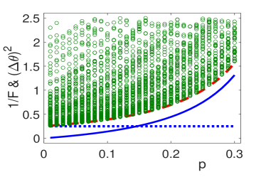
In the second example, we take instead of as the signal Hamiltonian to account the effect of decoherence. is calculated with , while the Hermitian Fisher information is calculated with ,
| (16) |
The scaling of Fisher information with the particle number remains unchanged, indicating there is no significant enhancement to parameter estimation in this example.
Saturation of the bounds and feasible experiments to measure an non-Hermitian variable.— To saturate the bounds, the optimal measurement has to meet and simultaneously supp . These requirements can not be satisfied for bound , as is Hermitian but is not as we stated earlier. Even if we lift the constrain on the Hermiticity of , the bound can not be saturated too due to the requirement of . This claim is confirmed by our numerical simulation, see Supplemental Material supp . The situation is different for bound . Simple analyses show that the measurement variable
| (17) |
with real can saturate the bound supp . For the example with trapped ions, can be measure in a single-shot experiment in an interferometer setup supp .
Conclusions.—The framework of quantum mechanics in which observable are associated with Hermitian operators is too narrow to discuss parameter estimation. Considering in the past two decades the non-Hermitian physics has attracted fast growing interest in various field of research, we first derived an uncertainty relation for non-Hermitian operators, then we deduce a previously unknown expression for non-Hermitian Fisher information. Two Cramér-Rao bounds that in some cases one of them, and sometimes both of them, are superior to the previous result are found. The saturation of these bounds is analysed and the optimal measurement to attain the bounds are given. The theory was illustrated with two experimentally feasible systems. The setup to measure non-Hermitian observables is also proposed.
We thank Xiaoming Lu for helpful discussions. This work was supported by the National Natural Science Foundation of China (NSFC) under Grants No. 11775048, and No. 12047566.
References
- (1) C. Helstrom, Minimum mean-squared error of estimates in quantum statistics, Phys. Lett. A 25, 101 (1967).
- (2) C. W. Helstrom, Quantum Detection and Estimation Theory, (Academic Press, New York, 1976).
- (3) A. S. Holevo, Probabilistic and Statistical Aspect of Quantum Theory, (North-Holland, Amsterdam, 1982).
- (4) C. L. Degen, F. Reinhard, and P. Cappellaro, Quantum sensing, Rev. Mod. Phys. 89, 035002(2017).
- (5) Luca Pezzè, Augusto Smerzi, Markus K. Oberthaler, Roman Schmied and Philipp Treutlein, Quantum metrology with nonclassical states of atomic ensembles, Rev. Mod. Phys. 90, 035005 (2018).
- (6) R. A. Fisher, Theory of Statistical Estimation, Proc. Camb. Soc. 22, 700 (1925).
- (7) Charles L. Matson and Alim Haji, Biased Cramér-Rao lower bound calculations for inequality-constrained estimators, J Opt Soc Am A 23,2702 (2006).
- (8) B. Roy Frieden, Fisher information, disorder, and the equilibrium distributions of physics, Phys. Rev. A 41, 4265(1990).
- (9) S. L. Braunstein, and C. M. Caves, Statistical distance and the geometry of quantum states, Phys. Rev. Lett. 72, 3439(1994).
- (10) Jing Liu, Haidong Yuan, Xiao-Ming Lu, Xiaoguang Wang, Quantum Fisher information matrix and multiparameter estimation, J. Phys. A: Math. Theor. 53, 023001 (2020).
- (11) Carl M. Bender and Stefan Boettcher, Real Spectra in Non-Hermitian Hamiltonians Having PT Symmetry, Phys. Rev. Lett. 80, 5243 (1998).
- (12) C. M. Bender, D. C. Brody, H. F. Jones, and B. K. Meister, Faster than Hermitian Quantum Mechanics, Phys. Rev. Lett. 98, 040403 (2007).
- (13) A. Guo, G. J. Salamo, D. Duchesne, R. Morandotti, M. Volatier-Ravat, V. Aimez, G. A. Siviloglou, and D. N. Christodoulides, Observation of PT-Symmetry Breaking in Complex Optical Potentials, Phys. Rev. Lett. 103, 093902 (2009).
- (14) V. V. Konotop, J. Yang, and D. A. Zezyulin, Nonlinear Waves in PT-Symmetric Systems, Rev. Mod. Phys. 88, 035002 (2016).
- (15) L. Feng, R. El-Ganainy, and L. Ge, Non-Hermitian Photonics Based on Parity-Time Symmetry, Nat. Photon. 11, 752 (2017).
- (16) R. El-Ganainy, K. G. Makris, M. Khajavikhan, Z. H. Musslimani, S. Rotter, and D. N. Christodoulides, Non-Hermitian Physics and PT Symmetry, Nat. Phys. 14, 11 (2018).
- (17) M.-A. Miri and A. Alú, Exceptional Points in Optics and Photonics, Science 363, eaar7709 (2019).
- (18) S. K. Özdemir, S. Rotter, F. Nori, and L. Yang, Parity-Time Symmetry and Exceptional Points in Photonics, Nat. Mater. 18, 783 (2019).
- (19) R. Hamazaki, K. Kawabata, and M. Ueda, Non-Hermitian Many-Body Localization, Phys. Rev. Lett. 123, 090603 (2019).
- (20) M. V. Berry, Physics of Nonhermitian Degeneracies, Czech. J. Phys. 54, 1039 (2004).
- (21) W. D. Heiss, The Physics of Exceptional Points, J. Phys. A 45, 444016 (2012).
- (22) N. Moiseyev, Non-Hermitian Quantum Mechanics, (Cambridge University Press, Cambridge, 2011).
- (23) H. P. Yuen and M. Lax, Multiple-Parameter Quantum Estimation and Measurement of Nonselfadjoint Observables, IEEE Trans. Inf. Theory 19 740 (1973).
- (24) J. Wiersig, Enhancing the Sensitivity of Frequency and Energy Splitting Detection by Using Exceptional Points: Application to Microcavity Sensors for Single-Particle Detection, Phys. Rev. Lett. 112, 203901 (2014).
- (25) Z.-P. Liu, J. Zhang, S. K. Özdemir, B. Peng, H. Jing, X.-Y. Lü, C.-W. Li, L. Yang, F. Nori, and Y.-X. Liu, Metrology with PT-Symmetric Cavities: Enhanced Sensitivity near the PT-Phase Transition, Phys. Rev. Lett. 117, 110802 (2016).
- (26) W. Chen, S. K. Özdemir, G. Zhao, J. Wiersig, and L. Yang, Exceptional points enhance sensing in an optical microcavity, Nature 548, 192 (2017).
- (27) H. Hodaei, A. U. Hassan, S. Wittek, H. Garcia-Gracia, R. El-Ganainy, D. N. Christodoulides, and M. Khajavikhan, Enhanced sensitivity at higher-order exceptional points, Nature 548, 187 (2017).
- (28) P. Djorwe, Y. Pennec, and B. Djafari-Rouhani, Exceptional Point Enhances Sensitivity of Optomechanical Mass Sensors, Phys. Rev. Applied 12, 024002(2019).
- (29) Xuan Mao, Guo-Qing Qin, Hong Yang, Hao Zhang, Min Wang, and Gui-Lu Long, Enhanced sensitivity of optical gyroscope in a mechanical parity-time-symmetric system based on exceptional point, New J. Phys. 22, 093009 (2020).
- (30) D. Leibfried, E. Knill, S. Seidelin, J. Britton, R. B. Blakestad, J. Chiaverini, D. B. Hume, W. M. Itano, J. D. Jost, C. Langer, R. Ozeri, R. Reichle and D. J. Wineland, Creation of a six-atom ‘Schrödinger cat’ state, Nature (London) 438, 639(2005).
- (31) Carlton M. Caves, Quantum-mechanical noise in an interferometer, Phys. Rev. D 23, 1693(1981).
- (32) A. W. Chin, S. F. Huelga, and M. B. Plenio, Quantum Metrology in Non-Markovian Environments, Phys. Rev. Lett. 109, 233601 (2012).
- (33) R. Demkowicz-Dobrzański, M. Jarzyna, and J. Kolodyński, Quantum limits in optical interferometry, Progress in Optics 60, 345 (2015).
- (34) V. Giovannetti, S. Lloyd, L. Maccone, Advances in quantum metrology, Nature Photonics 5, 222(2011).
- (35) A. Luis, Breaking the weak Heisenberg limit, Phys. Rev. A 95, 032113(2017).
- (36) Kai Bai, Zhen Peng, Hong-Gang Luo, Jun-Hong An, Retrieving ideal precision in noisy quantum optical metrology, Phys. Rev. Lett. 123, 040402 (2019)
- (37) C. W. Helstrom, Cramér-Rao inequalities for operator-valued measures in quantum mechanics, Int. J. Theor. Phys. 8,361(1973).
- (38) See Supplemental Material for detailed discussions on the deviation of the error propagation, the derivation of the Fisher information and Cramé-Rao bounds, comparison between the non-Hermitian Fisher information and the Hermitian Fisher information with non-Hermitian signal Hamiltonian, the saturation of Cramé-Rao bounds as well as the measurement of non-Hermitian operators.
- (39) Jose D. H. Rivero, Li Ge, Pseudo-chirality: a manifestation of Noether’s theorem in non-Hermitian systems, Phys. Rev. Lett. 125, 083902 (2020).
- (40) Kok-Wei Bong, Nora Tischler, Raj B. Patel, Sabine Wollmann, Geoff J. Pryde, and Michael J. W. Hall, Strong Unitary and Overlap Uncertainty Relations: Theory and Experiment, Phys. Rev. Lett. 120, 230402 (2018).
- (41) Bing Yu, Naihuan Jing, and Xianqing Li-Jost, Strong unitary uncertainty relations, Phys. Rev. A 100, 022116 (2019).
- (42) Arun Kumar Pati, Uttam Singh, and Urbasi Sinha, Measuring non-Hermitian operators via weak values, Phys. Rev. A 92, 052120 (2015).
- (43) Gaurav Nirala, Surya Narayan Sahoo, Arun K. Pati, and Urbasi Sinha, Measuring average of non-Hermitian operator with weak value in a Mach-Zehnder interferometer, Phys. Rev. A 99, 022111 (2019).
- (44) Surya Narayan Sahoo, Sanchari Chakraborti, Arun K. Pati, and Urbasi Sinha, Quantum State Interferography, Phys. Rev. Lett. 125, 123601(2020).
- (45) Thomas Monz, Philipp Schindler, Julio T. Barreiro, Michael Chwalla, Daniel Nigg, William A. Coish, Maximilian Harlander, Wolfgang Hänsel, Markus Hennrich, and Rainer Blatt, 14-Qubit Entanglement: Creation and Coherence, Phys. Rev. Lett. 106, 130506 (2011).
- (46) Marcin Jarzyna and Rafal Demkowicz-Dobrzański, Quantum interferometry with and without an external phase reference, Phys. Rev. A 85, 011801(R)(2012).
- (47) Luigi Seveso, Matteo A. C. Rossi, and Matteo G. A. Paris, Quantum metrology beyond the quantum Cramér-Rao theorem Phys. Rev. A 95, 012111(2017).
Supplementary material for:
Cramér-Rao bound and quantum parameter estimation with non-Hermitian systems
This supplemental material provides detailed derivations and calculations for the results in the main text. We give numbers to the equations and figures here with ”S” in contrast with that in the main text, for example, Eq.(S1), Fig. S1. Numbers without ”S” refer to the items in the main text, e.g., Eq. (1), Fig. 1. This materials are organized as follows.
-
S1.
We derive two Cramé-Rao bounds from uncertainty relations of non-Hermitian operators.
-
S2.
Non-Hermitian Fisher information is defined and previously unknown expressions to calculate the Fisher information is given.
-
S3.
Two examples to illustrate the non-Hermitian Fisher information are presented.
-
S4.
We present discussion and comparison between the non-Hermitian Fisher information and the Hermitian Fisher information with non-Hermitian signal Hamiltonian.
-
S5.
We discuss the second example with the other beam splitter.
-
S6.
This section devotes to discussion of saturation of Cramé-Rao bounds defined by the non-Hermitian Fisher information.
-
S7.
We focus on the measurement of non-Hermitian operators. Detailed experimental proposal is given.
S1 S1. Uncertainly relation and Cramé-Rao bound for non-Hermitian system
The precision of parameter estimation is limited by the quantum Cramér-Rao bound (CRB), which was an extension of Cramér-Rao bound in classical statistics to quantum metrology. As an extension of classical method, CRB has a wide range of applications, meanwhile it lacks a direct physical picture. In this section, we would derive the quantum CRB from the uncertainty relations that root deeply in the quantum theory from the beginning of the last century.
Consider two linear operators , and a real parameter , for any state , the following relation holds,
| (S1) |
Simple algebra yields,
| (S2) |
Noticing regardless of being Hermitian or not, and is real as is Hermitian, we obtain
| (S3) |
Define and the same for , and note the commutation relation, we have
| (S4) |
This is the equation (not numbered) in the main text.
Although the proof is conducted for pure states, the uncertainty relation Eq.(S4) holds for mixed states. We prove this by introducing an ancilla , such that a mixed state can be purified to be
| (S5) |
and the state of the system is obtained by tracing over the ancilla, With this consideration, Eq. (S4) can be straightforwardly extended to the composite system consisting of the system and the ancilla,
| (S6) |
Here, is the identity operator of ancilla . Noticing and denoting with Tr representing the trace over the system, we finish the proof of the weaker uncertainly relation in the main text. The slightly stronger uncertainty relation in Eq.(1) with mixed states can be proved in a similar way.
In order to develop a Cramér-Rao bound for non-Hermitian systems, we first have to extend error propagation from Hermitian to non-Hermitian systems, see Eq.(2). Assume a quantum state depends on parameter , the expectation value of operator and its conjugate would then depend on the parameter. Let us discretize the parameter by The fluctuation is then,
| (S7) |
where , and () stand for probabilities. Expanding around as
and approximating up to the second order in (), we arrive at
| (S8) |
Here, . This is the error propagation in Eq.(2) of the main text.
With this error propagation, we now derive the non-Hermitian Cramér-Rao bound in Eq.(3). Introducing an operator , which is not required to be Hermitian, we have
| (S9) | |||||
There are few differences between the present study and the earlier publications in , which deserve to be outlined. First, in most publications so far, is the so-called symmetric logarithmic derivative, which is required to be Hermitian. This requirement is due to the fact that the uncertainty relation used in the publications till now is for Hermitian operators. Whereas in our case is not required to be Hermitian. In fact, as we show in the main text an anti-Hermitian can maximize the Fisher information. Second, the uncertainty relation used to derive the Cramér bound is different, and our derivation can recover the results in the literature.
Until now, the operator is not required to be Hermitian. As we will show later, a non-Hermitian will lead a different Cramér-Rao bound.
Let us start to discuss a special case that is Hermitian. For Hermitian , the last line of Eq. (S9) becomes,
| (S10) | |||||
To have the last inequality, we have ignored , which is pure imaginary, while term is real. By carefully choosing , we can have Eq. (S9) reduces to Eq.(3) in the main text, where satisfies Eq.(4).
When is not Hermitian but with , we still obtain Eq. (3), but in this case, satisfies Eq. (5). The proof is almost the same as that for Eq. (4).
S2 S2. non-Hermitian quantum Fisher information
We present a detailed calculations for the Fisher information and defined in Eq. (3). We first calculate Without lose of generality, we assume the dimension of the Hilbert space is , while the state of the system may be not of full rank. It has positive eigenvalues required by quantum theory, and the corresponding eigenstates are denoted by , i.e.,
| (S13) |
Here we assume runs from to , . With these notations, the Fishier information defined in Eq.(3) takes,
| (S14) | |||||
Recalling Eq. (4) in the main text that,
| (S15) |
and assuming , we have
| (S16) |
As addressed in the main text, should not be limited to the space spanned by the eigenstates of , however for or , can not established by Eq. (S16). We will return to this point later. To compute , we need to know . Starting from Eq.(S13), we have
| (S17) |
leading to
| (S18) | |||||
Here, has been applied in the derivation. Substituting Eq.(S18) and Eq. (S16) into Eq. (S14), we have
| (S19) | |||||
where is the identity operator of the Hilbert space, i.e., . Note that the sum runs from 1 to . Finally, we obtain Eq. (8) in the main text,
can be derived by the same technique as employed in the derivation of . Note that , and for .
S3 S3. examples
Detailed calculation for the non-Hermitian quantum Fisher information and will be presented below. For mixed states of form with -independent , the Fisher information , and reduce to,
| (S21) |
In the first example, the state before encoding is
| (S22) |
The signal Hamiltonian used to encode the parameter into the state is , i.e., the encoding operation is given by . The states that carry the information of the parameter is then
| (S23) |
It is easy to find that
| (S24) |
Finally, we obtain Eq.(12) of the main text.
In the second example, the state before encoding is
| (S25) |
where denotes that both modes and are in its vacuum state. and was defined in the main text, i.e., , , and we will set . The parameter is encoded into the state after passing through a beam splitter represented by . The state encoding the parameter is then
| (S26) |
where , and Further, we find
| (S27) |
Collecting these results, we arrive at
| (S28) |
This is Eq.(14) in the main text. The dependence of the Fisher information on the photon number is depicted in Fig.S1.
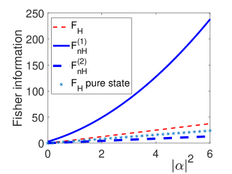
The Hermitian Fisher information for pure state is also shown for comparison with the others. We can clearly find that for large photon number, scales dominantly with , indicating the breakdown of the Heisenberg limit.
S4 S4. non-Hermitian signal Hamiltonian
In the following, we will consider a situation that the signal Hamiltonian is not Hermitian for . Comparison is carried out between the Hermitian quantum Fisher information with Hermitian signal Hamiltonian and the Hermitian quantum Fisher information with non-Hermitian signal Hamiltonian (will be denoted by ), and only the case of pure states is considered.
For pure state , , so we do not take into comparison. For pure states, and takes,
| (S29) | |||||
| (S30) |
where denotes the unnormalized encoding state and is its normalization constant, namely, . We might prove Eq.(S30) by substitution of into , and noticing
| (S31) |
In the first example, the signal Hamiltonian is replaced with , the encoding state would have the same form as in Eq.(S3) but with instead of . With these knowledge, we have
| (S32) |
which is Eq.(15) in main text.
One might wonder why the signal Hamiltonian takes instead of . This can be understood as follows. Consider the rotation applied to encode the parameter into the state. This rotation can be realized in trapped ionsmonz11 through an effective Hamiltonian ,
| (S33) |
where is a collective spin of those trapped ions, is the Rabi frequency of each ion or the magnetic field to which the ion coupled. The time evolution operator plays the role of the rotation operator. Here the accumulated phase
There is no quantum system being completely isolated from its surroundings including the trapped ions. A system that is coupled with its environment is called open system. A complete description of an open quantum system requires the inclusion of the environment. As a result of the interaction with the environment, the dynamics of the open system is governed by the master equationgardiner04 ,
| (S34) |
Consider a very short encoding time, terms with can be ignored. And the dynamics of the open system is governed by an effective Hamiltonian
| (S35) |
Consider each ion being modelled by a two-level system, the terms would contribute to as . Namely, in this open system
| (S36) |
Here stands for the decay rate of collective spin .
S5 S5. results with the other beam splitter
In Sec.S3, we employed a beam splitter, , in a standard Mach-Zehnder setup to study the Fisher information. With beam splitter , the mode (or mode ) is simply transmitted to another mode (or mode ), so there is no interferometer at all, the Fisher information is however not zero jarzyna12 . In the following, we will employ the other beam splitter, , to study the Fisher information. Involved but straightforward calculations show that,
| (S38) |
Here stands for the real part of . Substituting Eq.(S5) into Eqs(S3), we obtain the Fisher information of states with beam splitter . Numerical results are presented in Fig. S3. We find that except . This is similar to the results in Fig. 2 of the main text.
S6 S6. Saturation of non-Hermitian quantum Cramér-Rao bounds and
The variance of the estimated parameter is given by the error propagation Eq.(2) of the main text, it is bounded by the quantum Cramér-Rao bound (QCRB) defined through the quantum Fisher information as
Given a signal Hamiltonian and initial state, the bounds can be saturated by carefully chosen measurements characterized by variable (operator) . In the following, we will show that the bound given by can be saturated, while can not. The optimal measurement to saturate the bound is also given.
Recalling the Cauchy-Schwarz inequality, and noticing the equality holds if and only if ( is a constant) we claim that to saturate the bounds, ( is a constant). In other words, to reach the lower Cramér-Rao bound, the optimal measurement variable is required to be proportional to the symmetric logarithmic derivative .
In Eq. (S10), a term had been ignored in order to have the last inequality. For the equality to hold, is required, this together with require that is real. This means that to saturate the bounds, and must be Hermitian or non-Hermitian simultaneously. This suggests that bound can not be saturated, as is Hermitian but is not as we stated in the main text. In addition, can not be met as discussed in the main text.
As to the bound given by , all requirements for saturation are met, and the optimal measurement can be expressed in terms of the encoding state . Firstly, and can be met simultaneously, and there are no contradictions with the requirement in the main text. Secondly, from and Eq. (S12), we find that
| (S39) |
where, and are the eigenvalues and its corresponding eigenstates of the encoding state , respectively.
To be specific, we assume to be -independent as we did in the main text, then
| (S40) |
We apply these results to the first example, and find that the operators given in Eq. (S6) indeed saturate the bound , see Fig. S4. The saturation of bound is also presented for comparison, see Fig. S5.
We would like to notice that for , the bounds and are almost same, while remains unchanged. See Fig. S6. For the bounds and the variance behave similarly with respect the those in the region of .
From Figures S4, S5 and S6 we find that the bound plays no role yet in constraint on the parameter estimation. To show the role that plays, we examine the Mach-Zehnder setup with splitter. The results are presented in Fig. S7. The circles in the region enclosed by the red-dashed, blue-solid and the blue-dashed lines (i.e., the region with dotted ellipse) break the constraint by and while they are above the lower bound given by .
S7 S7. Measuring the average of a non-Hermitian operator
The key point of parameter estimation with non-Hermitian systems is to measure the average of non-Hermitian operator . In this section, we follow the proposal in Refs pati15 ; nirala19 ; abbott19 ; sahoo20 to show how to measure the non-Hermitian operator in our case.
Let us consider a non-Hermitian operator . The expectation value of in a quantum state given by is complex in general. This makes the non-Hermitian operator unobservable in experiments. Nevertheless, recent studies shown that this obstacle can be overcome with the help of polar decomposition hall15 , which states that given any operator , we can always decompose as with being an unitary operator and a Hermitian semidefinite operator, This bridges the average of non-Hermitian operator and the weak value of Hermitian operator as follows,
| (S41) |
where It is Well-known that is a weak value of the positive-semidefinite operator , which can be measured directly in the weak measurement aharonov88 .
In fact, the weak measurement is not necessary for the weak value and the average of non-Hermitian operator —they can be given in a single-shot measurement with an interferometric technique reported in sahoo20 . Before going into details of such a technique, we first show how to decompose the non-Hermitian operator in our first model.
To simplify the representation, let us consider a single trapped ion. For such a system, any non-Hermitian operator can be written as,
| (S42) |
where are complex parameters in general, and It is easy to find that
| (S43) |
where can be written in terms of and are all real since is Hermitian. Namely, and denote the real and imaginary part of Simple algebra yields the eigenstates and the corresponding eigenvalues of ,
| (S44) |
Here, and Then we have, leading to the decomposition,
| (S45) |
Note that as is Hermitian and positive. This observation together with leads to
| (S46) |
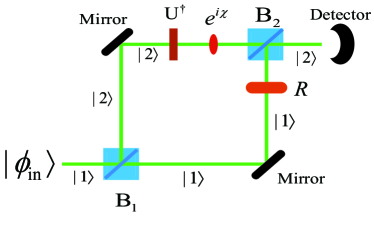
With the decomposition , Eq. (S45) and Eq. (S46), we now go to the measurement of non-Hermitian operator . The schematic setup is illustrated in Fig. S8. The average of in state , can be readout from the average intensity measured by the detector.
One point deserved to be addressed is that this set up can work for both polarized photons and two-level atoms. So, we would not specify which interferometer it is (Mach-Zehnder or Ramsey). In bases spanned by (), these operation can be written as
| (S55) | |||||
| (S64) |
where , and similar denotations hold for and With the same bases, the input state that only occupies spatial state takes,
| (S69) |
The output state reads
| (S70) |
simple algebra yields,
| (S75) |
The intensity the detector measures can be represented by
| (S76) |
with
| (S77) |
leading to
| (S78) |
where is the argument of , i.e., In experiment, the intensity together with which is the average of Hermitian operator can determine the average of non-Hermitian operator as both and can be inferred from the intensity .
References
- (1) Thomas Monz, Philipp Schindler, Julio T. Barreiro, Michael Chwalla, Daniel Nigg, William A. Coish, Maximilian Harlander, Wolfgang Hänsel, Markus Hennrich, and Rainer Blatt, 14-Qubit Entanglement: Creation and Coherence, Phys. Rev. Lett. 106, 130506 (2011).
- (2) C. W. Gardiner, and P. Zoller, Quantum Noise, (Berlin Heidelberg, Springer, 2004).
- (3) Marcin Jarzyna and Rafal Demkowicz-Dobrzański, Quantum interferometry with and without an external phase reference, Phys. Rev. A 85, 011801(R)(2012).
- (4) Arun Kumar Pati, Uttam Singh, and Urbasi Sinha, Measuring non-Hermitian operators via weak values, Phys. Rev. A 92, 052120 (2015).
- (5) Gaurav Nirala, Surya Narayan Sahoo, Arun K. Pati, and Urbasi Sinha, Measuring average of non-Hermitian operator with weak value in a Mach-Zehnder interferometer, Phys. Rev. A 99, 022111 (2019).
- (6) A. A. Abbott, R. Silva, J. Wechs, N. Brunner, and C. Branciard, Anomalous weak values without post-selection, Quantum 3, 194 (2019).
- (7) Surya Narayan Sahoo, Sanchari Chakraborti, Arun K. Pati, and Urbasi Sinha, Quantum State Interferography, Phys. Rev. Lett. 125, 123601(2020).
- (8) B. C. Hall, Lie Groups, Lie Algebras, and Representations: An Elementary Introduction (Springer, New York, 2015).
- (9) Yakir Aharonov, David Z. Albert, and Lev Vaidman, How the result of a measurement of a component of the spin of a spin-1/2 particle can turn out to be 100, Phys. Rev. Lett. 60, 1351(1988).