CP² Skyrmions and Skyrmion Crystals in Realistic Quantum Magnets

Lord Kelvin’s vision of the atom as a vortex in ether [1] inspired Skyrme [2, 3] to explain the origin of nucleons as emergent topologically non-trivial configurations of a pion field described by a 3+1 dimensional O(4) non-linear $\sigma$-model. In the modern language, these “skyrmions” are examples of topological solitons and Skyrme’s model has become the prototype of a classical theory that supports these solutions. Besides its important role in high-energy physics and cosmology, Skyrme’s model also led to important developments in other areas of physics. For instance, the baby Skyrme model [4, 5, 6] (planar reduction of the non-linear $\sigma$-model), which is as an extension of the Heisenberg model [4, 5, 7], has baby skyrmion solutions in the presence of a chiral symmetry breaking Dzyaloshinskii-Moriya (DM) interaction [8, 9, 10, 11].

Periodic arrays of magnetic skyrmions and single skyrmion metastable states were originally observed in chiral magnets, such as MnSi, Fe_1-xCo_xSi, FeGe and Cu₂OSeO₃ [12, 13, 14, 15, 16]. This discovery sparked the interest of the community at large and spawned efforts in multiple directions. Identifying realistic conditions for the emergence of novel magnetic skyrmions is one of the main goals of modern condensed matter physics. Novel mechanisms are usually accompanied by new properties. For instance, while skyrmions of chiral magnets have a fixed vector chirality, this is still a degree of freedom in centrosymmetric materials, such as BaFe_1-x-0.05Sc_xMg_0.05O₁₉, La_2-2xSr_1+2xMn₂O₇, Gd₂PdSi₃ and Gd₃Ru₄Al₁₂ [17, 18, 19, 20, 21, 22, 23], where skyrmions arise from frustration, i.e., from competing exchange or dipolar interactions [24, 25, 26, 27, 28, 29, 30].

The target manifold of the above-mentioned planar baby skyrmions is $S^{2}\cong$ CP¹, i.e., the usual 2D sphere, corresponding to normalized dipoles. More generally, one may consider the complex projective space CP^N-1 that represents the normalized $N$-component complex vectors, up to an irrelevant complex phase. The topologically distinct, smooth mappings from the base manifold $S^{2}$ (2D sphere $\cong$ compactified plane) to the target manifold CP^N-1 can be labeled by the integers: $\Pi_{2}(\mathrm{CP}^{N-1})=\mathbb{Z}$. This homotopy group suggests generalizations of the planar Skyrme’s model to $N>2$, such as the CP² non-linear $\sigma$-model [31, 32, 33] and in the Faddeev-Skyrme type model [34, 35]. In recent work, Akagi et al. considered the SU(3) version of the Heisenberg model with a DM interaction, whose continuum limit becomes a gauged CP² nonlinear $\sigma$-model with a background uniform gauge field [36]. An attractive aspect of this model is that it admits analytical solution by the application of techniques developed for the gauged non-linear $\sigma$-model. However, it may be challenging to find materials described by this model because SU(3) can only be an accidental symmetry of spin-spin interactions of real quantum magnets.

The main purpose of this work is to demonstrate that exotic CP² skyrmions readily emerge in simple and realistic spin-$1$ ($N=3$) models and their higher-spin generalizations. Remarkably, isolated CP² skyrmions can either be metastable states of a quantum paramagnet (QPM) or of a fully polarized (FP) ferromagnet. Unlike the “usual” CP¹ magnetic skyrmions, the dipolar field of the metastable CP² skyrmions of quantum paramagnets vanishes away from the skyrmion core. Moreover, the application of an external magnetic field to the QPM induces stable triangular crystals of CP² skyrmions in the field interval that separates the QPM from the FP state.

To illustrate the basic ideas we consider a minimal spin-$1$ model defined on the triangular lattice (TL):

$$\!\!\!{\hat{\mathcal{H}}}=\sum_{\langle i,j\rangle}J_{ij}\left({\hat{S}}^{x}_{i}{\hat{S}}^{x}_{j}+{\hat{S}}^{y}_{i}{\hat{S}}^{y}_{j}+\Delta{\hat{S}}^{z}_{i}{\hat{S}}^{z}_{j}\right)-h\sum_{i}{\hat{S}}^{z}_{i}+D\sum_{i}\left({\hat{S}}^{z}_{i}\right)^{2}.$$

(1)

The first term includes an easy-axis ferromagnetic (FM) nearest-neighbor exchange interaction $J_{1}<0$ and a second-nearest-neighbor antiferromagnetic (AFM) exchange $J_{2}>0$. For simplicity, we assume that the exchange anisotropy, defined by the dimensionless parameter $\Delta>1$, is the same for both interactions. The second and third terms represent the Zeeman coupling to an external field and an easy-plane single-ion anisotropy ($D>0$), respectively. $\hat{\mathcal{H}}$ is invariant under the space-group of the TL and the U(1) group of global spin rotations along the field-axis. We will adopt $|J_{1}|$ as the unit of energy (i.e. $J_{1}=-1$).

The first step is to take the classical limit of $\hat{\mathcal{H}}$, where multiple approaches are possible [37, 38]. The traditional classical limit is based on SU(2) coherent states, which retains only the spin dipole expectation value, and produces the Landau-Lifshitz spin dynamics. This approach is adequate for modeling systems with weak single-ion anisotropy $D\ll|J_{1}|$. To model systems in the regime $D\gtrsim|J_{1}|$, and correctly capture low-energy excitations, it is important to retain more information about spin fluctuations in the $(N=3)$-dimensional local Hilbert space. Specifically, our classical limit will assume that the many-body quantum state is a direct product of SU(3) coherent states [39, 37, 40, 41, 42, 43, 38]:

$$|\bm{Z}\rangle=\otimes_{j}|\bm{Z}_{j}\rangle\;\;{\rm with}\;\;|\bm{Z}_{j}\rangle=\sum_{a}Z^{a}_{j}\left|x^{a}\right\rangle_{j},$$

(2)

where $\bm{Z}_{j}=\left(Z^{1}_{j},Z^{2}_{j},Z^{3}_{j}\right)^{\mathrm{T}}$ is a complex vector of unit length and $\{\left|x^{1}\right\rangle_{j},\left|x^{2}\right\rangle_{j},\left|x^{3}\right\rangle_{j}\}$ is an orthonormal basis for the local Hilbert state on site $j$.

Local physical operators are represented by Hermitian matrices that act on SU(3) coherent states. The space of $3\times 3$ traceless, Hermitian matrices comprises the fundamental representation of the $\mathfrak{su}(3)$ Lie algebra. A basis $\hat{T}^{\mu}$ ($\mu=1,\dots,8$) for this space is characterized by the commutation relations,

$$\left[{\hat{T}}_{j}^{\eta},{\hat{T}}^{\mu}_{j}\right]=if_{\eta\mu\nu}{\hat{T}}_{j}^{\nu},$$

(3)

where we are using the convention of summation over repeated Greek indices. We may additionally impose an orthonormality condition

$$\operatorname{Tr}\left({\hat{T}}_{j}^{\alpha}{\hat{T}}_{j}^{\beta}\right)=2\delta_{\alpha\beta}.$$

(4)

It is conventional to define the structure constants as $f_{\eta\mu\nu}=-\frac{i}{2}\operatorname{Tr}\left({\lambda}_{\eta}\left[{\lambda}_{\mu},{\lambda}_{\nu}\right]\right),$ where ${\lambda}_{\mu}$ are the Gell-Mann matrices.

The spin dipole operators $\hat{\bm{S}}_{j}=(\hat{S}^{x}_{j},\hat{S}^{y}_{j},\hat{S}^{z}_{j})^{T}$ acting on site $j$ are generators for a spin-$1$ representation of SU(2). It is possible to formulate generators of SU(3) as polynomials of these spin operators,

$\displaystyle\left(\begin{array}[]{l}{\hat{T}}_{j}^{7}\\ {\hat{T}}_{j}^{5}\\ {\hat{T}}_{j}^{2}\end{array}\right)=-\left(\begin{array}[]{c}{\hat{S}}_{j}^{x}\\ {\hat{S}}_{j}^{y}\\ {\hat{S}}_{j}^{z}\end{array}\right),\left(\begin{array}[]{l}{\hat{T}}_{j}^{3}\\ {\hat{T}}_{j}^{8}\\ {\hat{T}}_{j}^{1}\\ {\hat{T}}_{j}^{4}\\ {\hat{T}}_{j}^{6}\end{array}\right)=\left(\begin{array}[]{c}-\left({\hat{S}}_{j}^{x}\right)^{2}+\left({\hat{S}}_{j}^{y}\right)^{2}\\ \frac{1}{\sqrt{3}}\left[3\left({\hat{S}}_{j}^{z}\right)^{2}-{\hat{\bm{S}}}_{j}^{2}\right]\\ {\hat{S}}_{j}^{x}{\hat{S}}_{j}^{y}+{\hat{S}}_{j}^{y}{\hat{S}}_{j}^{x}\\ -{\hat{S}}_{j}^{z}{\hat{S}}_{j}^{x}-{\hat{S}}_{j}^{x}{\hat{S}}_{j}^{z}\\ {\hat{S}}_{j}^{y}{\hat{S}}_{j}^{z}+{\hat{S}}_{j}^{z}{\hat{S}}_{j}^{y},\end{array}\right),$

(21)

where $T_{j}^{7,5,2}$ are the dipolar components of the spin-1 degree of freedom, while the other five generators are the quadrupolar components. Here we have adopted the notation and conventions of Ref. [36] to make closer contact with the literature on high-energy physics ¹¹1Our definitions for $\hat{S}^{x}$ and $\hat{S}^{z}$ differ from these two in Ref [36] by a minus sign..

Let $|1\rangle_{j}$, $|0\rangle_{j}$, and $|\bar{1}\rangle_{j}$ denote the normalized eigenstates of ${\hat{S}}^{z}_{j}$, with eigenvalues, 1, 0 and -1, respectively. In the Cartesian basis,

$$\left|x^{1}\right\rangle_{j}=\frac{i\left[|1\rangle_{j}-|\bar{1}\rangle_{j}\right]}{\sqrt{2}},\left|x^{2}\right\rangle_{j}=\frac{\left[|1\rangle_{j}+|\bar{1}\rangle_{j}\right]}{\sqrt{2}},\left|x^{3}\right\rangle_{j}=-i|0\rangle_{j},$$

(22)

the SU(3) generators given in Eq. (21) are the Gell-Mann matrices:

$$\langle x^{a}_{j}|{\hat{T}}_{j}^{\mu}|x^{b}_{j}\rangle=\left({\lambda}_{\mu}\right)_{ab}\quad\mu=1,2,\cdots,8.$$

(23)

The orbit of coherent states $|\bm{Z}_{j}\rangle$ is obtained by applying SU(3) transformations to the highest weight state $|1\rangle_{j}$ [37]: $|\bm{Z}_{j}\rangle={\hat{U}}_{j}|1\rangle_{j}$. Since the global phase is a gauge degree of freedom, the orbit of physical SU(3) coherent states is $S^{5}/S^{1}\cong\mathrm{CP}^{2}$. The “SU(3) classical limit” of the spin Hamiltonian (1) is obtained by replacing the Hamiltonian operator ${\hat{\mathcal{H}}}$ with its expectation value

$${\cal H}\equiv\langle\bm{Z}|{\hat{\mathcal{H}}}|\bm{Z}\rangle,$$

(24)

after rewriting ${\hat{\mathcal{H}}}$ in terms of SU(3) spin components,

$${\hat{\mathcal{H}}}=\sum_{\langle i,j\rangle}{I}^{\mu}_{ij}{\hat{T}}^{\mu}_{i}{\hat{T}}^{\mu}_{j}-\sum_{i}B^{\mu}{\hat{T}}^{\mu}_{i},$$

(25)

where ${I}^{\mu}_{ij}=J_{ij}(\Delta\delta_{\mu,2}+\delta_{\mu,5}+\delta_{\mu,7})$ and $B^{\mu}=(-h\delta_{\mu,2}-D\delta_{\mu,8}/\sqrt{3})$. Because of the direct product form of Eq. (2), ${\cal H}$ can be expressed as a function of the “color field”

$$n^{\mu}_{j}\equiv\langle\bm{Z}_{j}|{\hat{T}}_{j}^{\mu}|\bm{Z}_{j}\rangle=\left({\lambda}_{\mu}\right)_{ab}\bar{Z}^{a}_{j}Z^{b}_{j},$$

(26)

which satisfies the constraints

$$n^{\mu}n^{\mu}=\frac{4}{3},\quad n^{\mu}=\frac{3}{2}d_{\mu\nu\eta}n^{\nu}n^{\eta},$$

(27)

where $d_{\mu\nu\eta}=\frac{1}{4}\operatorname{Tr}\left(\lambda_{\mu}\left\{\lambda_{\nu},\lambda_{\eta}\right\}\right)$. This in turn leads to the Casimir identity: $d_{mpq}n^{m}n^{p}n^{q}=\frac{8}{9}.$ In terms of this color field, we can express

$${\mathcal{H}}=\sum_{\langle i,j\rangle}{I}^{\mu}_{ij}{n}^{\mu}_{i}{n}^{\mu}_{j}-\sum_{i}B^{\mu}{n}^{\mu}_{i}.$$

(28)

To avoid an explicit use of the structure constants ($f_{\eta\mu\nu}$), we introduce the operator field $\bm{\mathfrak{n}}_{j}=n^{\mu}_{j}{\lambda}_{\mu}$. Topological soliton solutions of the color field become well-defined in the continuum (long wavelength) limit, where the Hamiltonian can be approximated by

$$\mathcal{H}\simeq\int\mathrm{d}r^{2}\left[-\frac{{\cal I}^{\mu}_{1}}{2}\partial_{a}{n}^{\mu}\partial_{a}{n}^{\mu}+\frac{{\cal I}^{\mu}_{2}}{2}\left(\nabla^{2}{n}^{\mu}\right)^{2}-\mathcal{B}^{\mu}n^{\mu}\right].$$

(29)

Here $\partial_{a}$ denotes the spatial derivatives and there is an implicit summation over the repeated $a$ index. The coupling constants can be expressed in terms of the parameters of the lattice model (25):

	$\displaystyle{\cal I}^{\mu}_{1}$	$\displaystyle=$	$\displaystyle\frac{3}{2}({I}^{\mu}_{1}+3{I}^{\mu}_{2}),\quad{\cal I}^{\mu}_{2}=\frac{3}{32}(I^{\mu}_{1}+9I^{\mu}_{2}),$
	$\displaystyle{\cal B}^{\mu}$	$\displaystyle=$	$\displaystyle B^{\mu}-3(\Delta-1)(J_{1}+J_{2})\delta_{\mu,8}.$		(30)

Eq. (29) corresponds to an anisotropic CP² model. For skyrmion solutions the base plane $\mathbb{R}^{2}$ can be compactified to $S^{2}$ because the color field takes a constant value $n_{\infty}$ at spatial infinity. These spin textures can then be characterized by the topological charge of the mapping $\bm{\mathfrak{n}}:\mathbb{R}^{2}\sim S^{2}\mapsto CP^{2}$:

$$C=-\frac{i}{32\pi}\int\mathrm{d}x\mathrm{d}y\varepsilon_{jk}\operatorname{Tr}\left(\bm{\mathfrak{n}}\left[\partial_{j}\bm{\mathfrak{n}},\partial_{k}\bm{\mathfrak{n}}\right]\right).$$

(31)

For the lattice systems of interest, the CP² skyrmion charge can be computed after interpolating the color fields on nearest-neighbor sites $\bm{\mathfrak{n}}_{j}$ and $\bm{\mathfrak{n}}_{k}$ along the CP² geodesic:

$$C=\sum_{\triangle_{jkl}}\rho_{jkl}=\frac{1}{2\pi}\sum_{\triangle_{jkl}}\left(\gamma_{jl}+\gamma_{lk}+\gamma_{kj}\right),$$

(32)

where $\triangle_{jkl}$ denotes each oriented triangular plaquette of nearest-neighbor sites $j\to k\to l$ and $\gamma_{kj}=\arg\left[\left\langle\bm{Z}_{k}\mid\bm{Z}_{j}\right\rangle\right]$ is the Berry connection on the bond $j\to k$ [45].

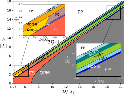
The $T=0$ phase diagram is obtained by numerically minimizing the classical spin Hamiltonian $\mathcal{H}$ (28) in the $4L^{2}$-dimensional phase space of a magnetic cell of $L\times L$ spins (see Methods). The shape and size of this unit cell is dictated by the symmetry-related magnetic ordering wave vectors $\bm{Q}_{\nu}$ ($\nu=1,2,3$) [see Figs. 2a and b], which are determined by minimizing the exchange interaction in momentum space: $J({\bm{q}})=\sum_{jl}J_{jl}e^{{i\mkern 1.0mu}\bm{q}\cdot(\bm{r}_{j}-\bm{r}_{l})}.$ The ratio between both exchange interactions, $J_{2}/|J_{1}|=2/(1+\sqrt{5})$, is tuned to fix the magnitude of the ordering wave vectors, $|\bm{Q}_{\nu}|=|\bm{b}_{1}|/5$ [27], corresponding to a magnetic unit cell of linear size $L=5$. A we will see later, the relevant qualitative aspects of the phase diagram do not depend on the particular choice of the model. The three ordering wave vectors, which are related by the $C_{6}$ symmetry of the TL, are parallel to the $\Gamma$-M_ν directions (denoted in Fig. 2).

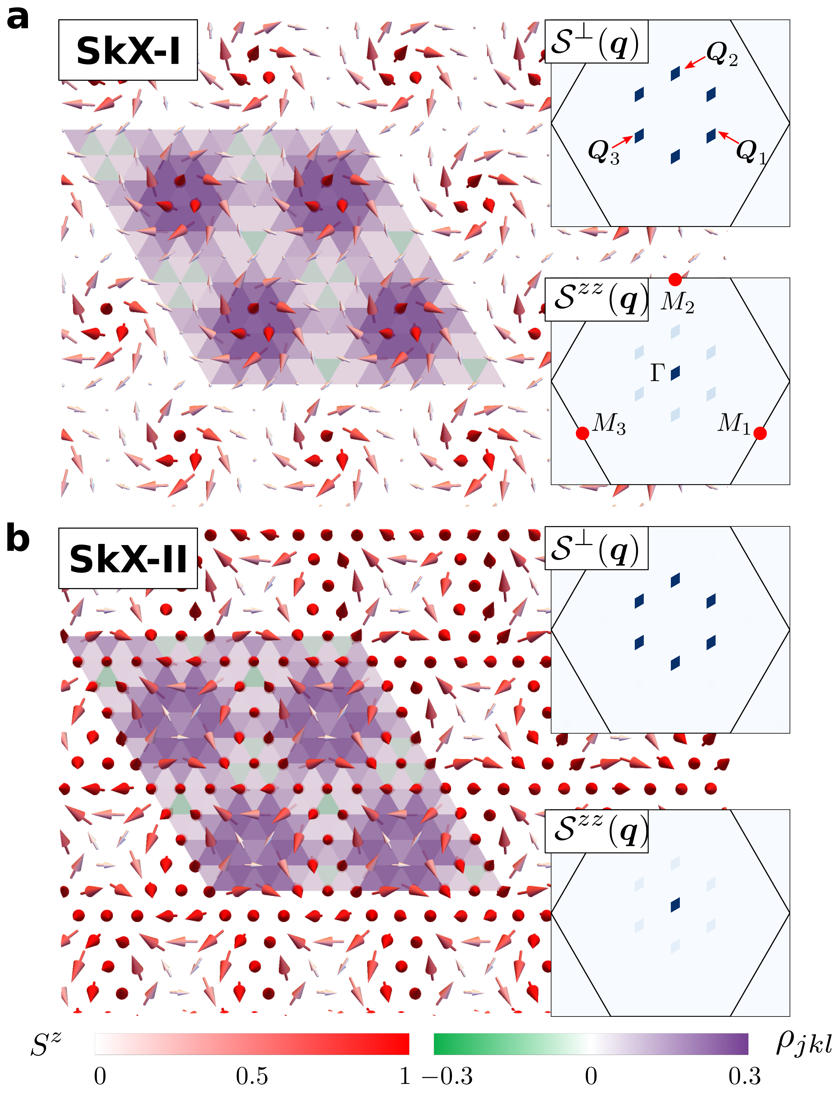
The resulting phase diagram shown in Fig. 1 includes multiple magnetically ordered phases between the FP phase and the QPM phase, where every spin is in the $|0\rangle$ state. For $D\gg|J_{1}|$, these phases include two field-induced CP² skyrmion crystals (SkX-I and SkX-II), separated by two modulated vertical spiral phases (MVS-I and MVS-II), where the polarization plane of the spiral is parallel to the $c$-axis and the magnitude of the dipole moment is continuously suppressed as the moment rotates from $\hat{\bm{z}}$ to $-\hat{\bm{z}}$ directions. The spiral phases have the same symmetry and are separated by a first order metamagnetic transition. As shown in Fig. 2a, the CP² skyrmions of the SkX-I crystal have dipole moments that evolve continuously into the purely nematic state ($|0\rangle$) as they move away from the core. Conversely, Fig. 2b shows that the spins in the SkX-II phase have a strong quadrupolar character (the small dipolar moment is completely suppressed in the large $D/|J_{1}|$ limit) at the skyrmion core, and evolve continuously into the magnetic state $|1\rangle$ as they move away from the core. The CP² skyrmion density distribution $\rho_{jkl}$ is also indicated with colored triangular plaquettes in Fig. 2a, b for SkX-I and SkX-II, respectively. As shown in the inset of Fig. 1, the phase SkX-II extends down to $D/|J_{1}|\simeq 5$, while the phase SkX-I disappears near $D/|J_{1}|\simeq 8$.

New competing orderings appear in intermediate $D/|J_{1}|$ region. In particular, a significant fraction of the phase diagram is occupied by the so-called canted spiral (CS) phase,

$$|\bm{Z}_{j}\rangle=\cos\theta|0\rangle_{j}+e^{i\bm{Q}\cdot\bm{r}_{j}}\sin\theta\cos\phi|1\rangle_{j}+e^{-i\bm{Q}\cdot\bm{r}_{j}}\sin\theta\sin\phi|\bar{1}\rangle_{j},$$

(33)

where $\theta$ and $\phi$ are variational parameters, and $\bm{Q}$ can take any values among {$\bm{Q}_{1}$, $\bm{Q}_{2}$, $\bm{Q}_{3}$}. Upon increasing $D$, the magnitude of the dipole moment of each spin, $|\langle\hat{\bm{S}}_{j}\rangle|$, is continuously suppressed to zero at the boundary,

$$D_{c}=h\sqrt{1-\frac{4J^{2}(\bm{Q})}{h^{2}+4J^{2}(\bm{Q})}}-2J(\bm{Q})\left(1-\frac{2J(\bm{Q})}{\sqrt{h^{2}+4J^{2}(\bm{Q})}}\right),$$

(34)

that signals the second order transition into the QPM phase. As shown in Fig. 1, several competing phases appear above the CS phase upon increasing $h$. These phases include three triple-$\bm{Q}$ spiral orderings [3$\bm{Q}$ I-III] with dominant weight in one of three $\bm{Q}$ transverse components and a staggered distribution of the CP² skyrmion density $\rho_{jkl}$ [see Eq. (32)] and three different modulated double-$\bm{Q}$ orderings (MDQ I - III) and two triple-$\bm{Q}$ orderings. All of these phases are described in detail in the supplementary information. In the rest of the paper we will focus on the SkX phases and the single-skyrmion metastable solutions that emerge in their proximity.

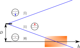
The origin of the CP² skyrmion crystals can be understood by analyzing the small $|J_{ij}|/D$ regime, where $\hat{\mathcal{H}}$ can be reduced via first order degenerate perturbation theory in $J_{ij}/D$ to an effective pseudo-spin-$1/2$ low-energy Hamiltonian,

$$\hat{\mathcal{H}}_{\text{eff}}=\sum_{\langle i,j\rangle}{\tilde{J}}_{ij}(\hat{s}^{x}_{i}\hat{s}^{x}_{j}+\hat{s}^{y}_{i}\hat{s}^{y}_{j}+\tilde{\Delta}\hat{s}^{z}_{i}\hat{s}^{z}_{j})-{\tilde{h}}\sum_{i}\hat{s}^{z}_{i}.$$

(35)

The pseudo-spin-$1/2$ operators are the projection of the original spin operators into the low-energy subspace ${\cal S}_{0}$ generated by the quasi-degenerate doublet $\{|0\rangle_{j},|1\rangle_{j}\}$ (see Fig. 3):

$$\hat{s}^{z}_{j}={\cal P}_{0}\hat{S}^{z}_{j}{\cal P}_{0}-\frac{1}{2},\quad\hat{s}^{\pm}_{j}=\frac{{\cal P}_{0}\hat{S}^{\pm}_{j}{\cal P}_{0}}{\sqrt{2}},$$

(36)

where ${\cal P}_{0}$ is the projection operator of the low-energy subspace. Importantly, the first state of the doublet has a net quadrupolar moment but no net dipole moment, $\langle 0|\hat{\bm{S}}_{j}|0\rangle_{j}=0$, while the second state maximizes the dipole moment along the $\hat{\bm{z}}$-direction $\langle 1|\hat{\bm{S}}_{j}|1\rangle_{j}=\hat{\bm{z}}$. This means that three pseudo-spin operators generate an SU(2) subgroup of SU(3) different from the SU(2) subgroup of spin rotations.

$\hat{\mathcal{H}}_{\text{eff}}$ represents an effective triangular easy-axis XXZ model with effective exchange, anisotropy and field parameters ${\tilde{J}}_{ij}=2J_{ij}$, $\tilde{\Delta}=\frac{\Delta}{2}$ and ${\tilde{h}}=h-D-3\Delta(J_{1}+J_{2})$, respectively. This model is known to exhibit a field-induced CP¹ SkX phase [25, 27] that survives in the long-wavelength limit [26]:

$$\mathcal{H}_{\text{eff}}\simeq\int\mathrm{d}r^{2}\left[-\frac{{\cal J}^{\eta}_{1}}{2}\partial_{a}\tilde{n}^{\eta}\cdot\partial_{a}\tilde{n}^{\eta}+\frac{{\cal J}^{\eta}_{2}}{2}\left(\nabla^{2}\tilde{n}^{\eta}\right)^{2}-\tilde{\cal B}\tilde{n}_{z}+\tilde{\cal D}\tilde{n}_{z}^{2}\right],$$

(37)

where $\eta=x,y,z$ denotes the three components of the unit vector field $\tilde{\bm{n}}$ ($|\tilde{\bm{n}}|=1$), and

	$\displaystyle{\cal J}^{\eta}_{1}$	$\displaystyle=$	$\displaystyle\frac{3s^{2}}{2}(\tilde{J}_{1}+3\tilde{J}_{2})[1+(\tilde{\Delta}-1)\delta_{\eta z}],$
	$\displaystyle{\cal J}^{\eta}_{2}$	$\displaystyle=$	$\displaystyle\frac{3s^{2}}{32}(\tilde{J}_{1}+9\tilde{J}_{2})[1+(\tilde{\Delta}-1)\delta_{\eta z}]$
	$\displaystyle\tilde{\cal B}$	$\displaystyle=$	$\displaystyle s{\tilde{h}},\quad\tilde{\cal D}=3s^{2}(\tilde{\Delta}-1)(\tilde{J}_{1}+\tilde{J}_{2}),$		(38)

where $s=1/2$. Although the target manifold of this theory is CP¹ (orbit of SU(2) coherent states that belong ${\cal S}_{0}$), we must keep in mind that $\hat{\mathcal{H}}_{\text{eff}}$ describes the large $D/|J_{1}|$ limit where the CP² skyrmions of the original spin-$1$ model become asymptotically close to CP¹ pseudo-spin skyrmions. In other words, the SkXs include a finite $|\bar{1}\rangle$ component for finite $D/|J_{1}|$, which increases upon decreasing $D$. This component, which only appears in the low-energy model when second order corrections in $J_{ij}$ are included, is responsible for the metamagnetic transition between the MVS-I and MVS-II phases (the transition disappears in the $D\to\infty$ limit).

Since $\hat{\mathcal{H}}_{\text{eff}}(h)$ and $\hat{\mathcal{H}}_{\text{eff}}(-h)$ are related by a pseudo-time-reversal (PTR) transformation ($\hat{s}_{j}\to-\hat{s}_{j}$ on the lattice and $\tilde{n}\to-\tilde{n}$ in the continuum) their corresponding ground states are related by the same transformation. In particular, the ground state $(\tilde{\bm{n}}=\hat{\bm{z}})$ that is obtained above the saturation field ($\tilde{\cal B}>\tilde{\cal B}_{\rm sat}$) corresponds to the FP state ($\langle\hat{\bm{S}}_{j}\rangle=\hat{\bm{z}}$) in the original spin-$1$ variables, while the ground state $(\tilde{\bm{n}}=-\hat{\bm{z}})$ below the negative saturation field ($\tilde{\cal B}<-\tilde{\cal B}_{\rm sat}$) corresponds to the QPM phase ($|\bm{Z}_{j}\rangle=|0\rangle_{j}$). Correspondingly, the SkX induced by a positive $h$ has pseudo-spins polarized along the quadrupolar direction ($|0\rangle$) near the core of the skyrmions and parallel to the dipolar one ($|1\rangle$) at the midpoints between two cores. This explains the origin of the SkX-II crystals depicted in Fig. 2 b. The negative ${\cal B}$ counterpart of this phase, which is obtained by applying the PTR transformation, corresponds to the SkX-I crystal shown in Fig. 2a. In this case the skyrmion cores are magnetic, while the midpoints are practically quadrupolar (they become purely quadrupolar in the large $D/|J_{1}|$ limit). This simple reasoning explains the origin of the novel SkX phases included in the $T=0$ phase diagram of $\mathcal{H}$ shown in Fig. 1. The intermediate phase between the SkX-I and SkX-II ground state of ${\mathcal{H}}$ induced by positive and negative values of $h$ is a single-$\bm{Q}$ spiral with a polarization plane parallel to the $c$-axis known as vertical spiral (VS). This explains the origin of the MVS-I and MVS-II phases in between the two SkX phases (the first order transition between both phases disappears in the large-$D$ limit [25]).

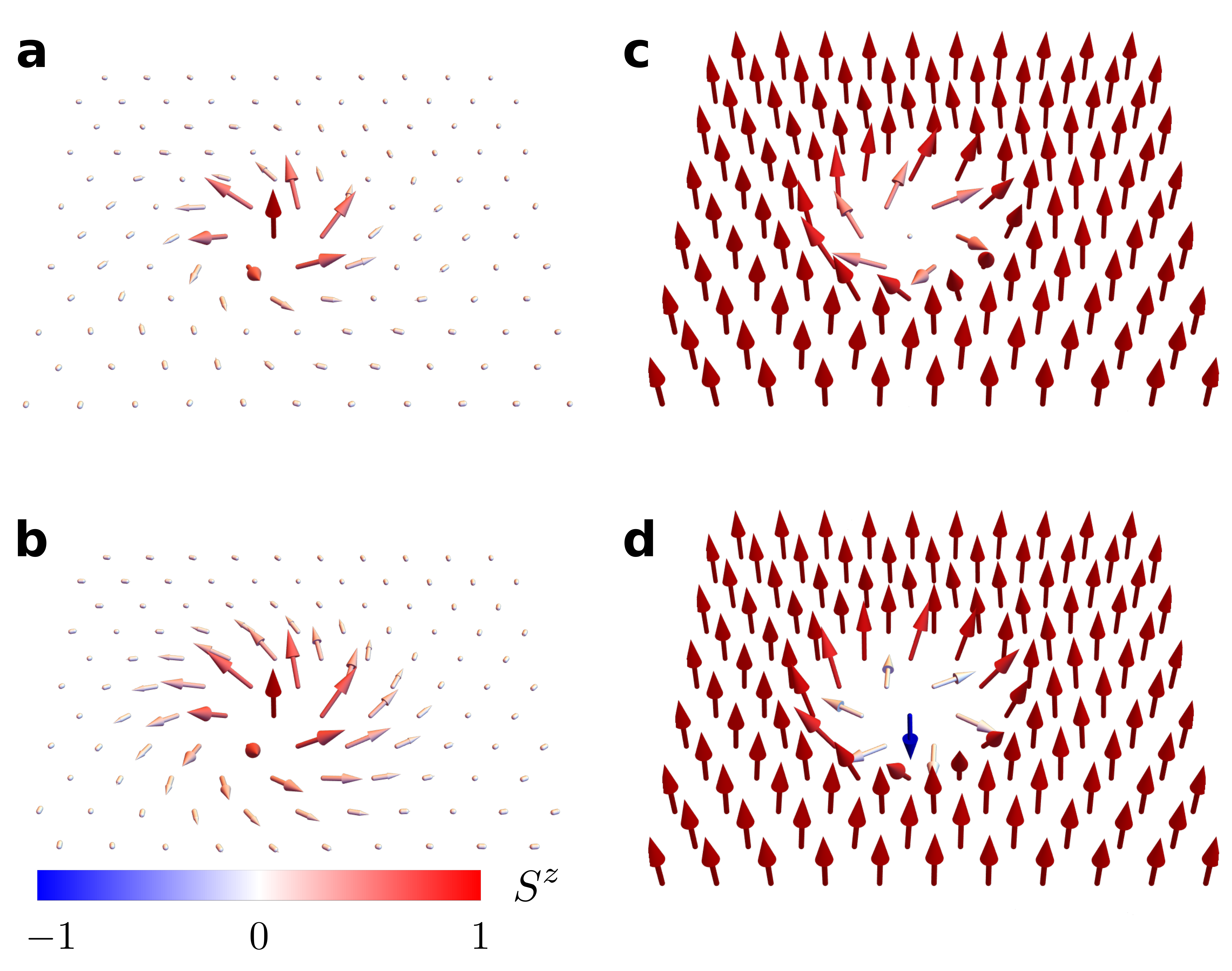
Single-skyrmion solutions. Besides the SkX phases shown in Fig. 4, the effective field theory (37) is known to support metastable CP¹ single-skyrmion solutions beyond the saturation fields $|\tilde{\mathcal{B}}|>\tilde{\mathcal{B}}_{\rm sat}$. The pseudo-spin variable is anti-parallel to the external field at the core and it gradually rotates towards the direction parallel to the field upon moving away from the center. Interestingly, this pseudo-spin texture translates into metastable single-skyrmion solutions of the QPM phase that have a magnetic core and a nematic periphery, as it is shown in Figs. 4a and b for different sets of Hamiltonian parameters. The CP² skyrmions are metastable solutions in the QPM phase for $D\gtrsim 14$, implying that these exotic magnetic-nematic textures should emerge in real magnets under quite general conditions.

Similarly, the metastable pseudo-spin single-skyrmion solutions of the FP phase ($\tilde{\mathcal{B}}>\tilde{\mathcal{B}}_{\rm sat}$) lead to a spin texture with a nematic (non-magnetic) core and a magnetic (FP) periphery, like the one shown in Fig. 4c. Interestingly, this exotic CP² skyrmion solution remains metastable down to $D\simeq 4|J_{1}|$ and it coexists with regular (CP¹) metastable skyrmion solutions, like the one shown Fig. 4d, that emerge below $D\simeq 4.25|J_{1}|$.

In summary, we have demonstrated that CP² skyrmion textures emerge in realistic models of hexagonal magnets out of the combination of geometric frustration with competing exchange and single-ion anisotropies. It is important to note that the skyrmion crystals and metastable solutions reported in this work survive in the long wavelength limit [26], implying that the above described CP² skyrmion phases should also exist in extensions of the model to honeycomb and Kagome lattice geometries. The generic spin-$1$ model considered in this work describes a series of triangular antiferromagnets in the form of ABX₃, BX₂, and ABO₂ [46, 47, 48], where A is a an alkali metal, B is a transition metal, and X is a halogen atom. Several Ni-based compounds, including NiGa₂S₄ [49], Ba₃NiSb₂O₉ [50], Na₂BaNi(PO₄)₂ [51], are also found to be realizations of spin-$1$ models on TLs. Some of these compounds have been already identified as candidates to host crystals of CP¹ magnetic skyrmions that are stabilized by the combination of frustration and exchange anisotropy [52]. Others, such as FeI₂ [53, 54], are described by the the Hamiltonian (1) but the sign of the single-ion and exchange anisotropies is opposite to the case of interest in this work. Related compounds, such as CsFeCl₃, are known to be quantum paramagnets described by the Hamiltonian (1) [55] with a dominant easy-plane single-ion anisotropy $D/J_{1}\simeq 10$. An alternative route to find realizations of our spin-$1$ Hamiltonian is to consider hexagonal materials comprising $4f$ magnetic ions with a singlet single-ion ground state and an excited Ising-like doublet (the effective easy-plane single-ion anisotropy $D$ is equal to the singlet-doublet gap). Ultracold atoms are also powerful platforms to realize spin-$1$ models with tunable single-ion anisotropy [56].

Our results demonstrate that magnetic field induced CP² skyrmion crystals should emerge in the presence of a dominant single-ion easy-plane anisotropy $D$ that is strong enough to stabilize a QPM at $T=0$. In terms of SU(3) spins, the single-ion anisotropy acts as an external SU(3) field that couples linearly to one component (${\hat{T}}_{j}^{8}$) of the quadrupolar moment. Correspondingly, the QPM can be regarded as a uniform quadrupolar state induced by a strong enough ${\hat{T}}_{j}^{8}$ component of the SU(3) field. The field-induced quantum phase transition between this uniform quadrupolar state and the skyrmion crystals is presaged by the emergence of metastable CP² single-skyrmion solutions consisting of a magnetic skyrmion core that decays continuously into a quadrupolar periphery. These novel skyrmions can be induced by increasing the strength of the magnetic field in the neighborhood of a given magnetic ion of a frustrated quantum paramagnet with competing exchange and single-ion anisotropies.

We acknowledge useful discussions with Xiaojian Bai, Antia Botana, Ying Wai Li, Shizeng Lin, Cole Miles, Martin Mourigal, Sakib Matin, Matthew Wilson, and Shang-Shun Zhang. D. D., K. B. and C.D.B. acknowledge support from U.S. Department of Energy, Office of Science, Office of Basic Energy Sciences, under Award No. DE-SC0022311. The work by H.Z. was supported by the Graduate Advancement, Training and Education (GATE) fellowship. Z.W. was supported by the U.S. Department of Energy through the University of Minnesota Center for Quantum Materials, under Award No. DE-SC-0016371.

The numerical minimization for the phase diagram Fig. 1 is done in a cell of $10\times 10$ spins containing four magnetic unit cells ($L=5$). Two crucial steps are useful to improve the efficiency of the local gradient-based minimization algorithms [57]. In the first step, we set multiple random initial conditions $|\bm{Z}\rangle$ ($\sim$ 50 for our case), where $|\bm{Z}_{j}\rangle$ on every site $j$ is uniformly sampled on the CP${}^{2}\simeq S^{5}/S^{1}$ manifold. After running the minimization algorithm, we keep the solution with the lowest energy for a given set of Hamiltonian parameters. In the next step, half of the initial conditions are randomly generated, while the other half correspond to the lowest-energy solutions obtained in the first step within a predefined neighborhood of the Hamiltonian parameters. This procedure is iterated until the phase diagram converges.

References

- [1] Thomson, W. Ii. on vortex atoms. London, Edinburgh, Dublin Philos. Mag. J. Sci. 34, 15–24 (1867). URL https://doi.org/10.1080/14786446708639836. eprint https://doi.org/10.1080/14786446708639836.
- [2] Skyrme, T. H. R. A non-linear field theory. Proc. R. Soc. A 260, 127–138 (1961). URL http://rspa.royalsocietypublishing.org/content/260/1300/127.abstract.
- [3] Skyrme, T. H. R. The origins of skymions. International Journal of Modern Physics A 3, 2745–2751 (1988). URL http://inis.iaea.org/search/search.aspx?orig_q=RN:21029176.
- [4] Bogolubskaya, A. & Bogolubsky, I. Stationary topological solitons in the two-dimensional anisotropic heisenberg model with a skyrme term. Physics Letters A 136, 485–488 (1989).
- [5] Bogolyubskaya, A. A. & Bogolyubsky, I. L. ON STATIONARY TOPOLOGICAL SOLITONS IN TWO-DIMENSIONAL ANISOTROPIC HEISENBERG MODEL. Lett. Math. Phys. 19, 171–177 (1990).
- [6] Leese, R., Peyrard, M. & Zakrzewski, W. Soliton scatterings in some relativistic models in (2+1) dimensions. Nonlinearity 3, 773–807 (1990).
- [7] Polyakov, A. M. & Belavin, A. A. Metastable States of Two-Dimensional Isotropic Ferromagnets. JETP Lett. 22, 245–248 (1975).
- [8] Dzyaloshinsky, I. A thermodynamic theory of weak ferromagnetism of antiferromagnetics. J. Phys. Chem. Solids 4, 241 (1958). URL http://www.sciencedirect.com/science/article/pii/0022369758900763.
- [9] Moriya, T. New mechanism of anisotropic superexchange interaction. Phys. Rev. Lett. 4, 228–230 (1960). URL http://link.aps.org/doi/10.1103/PhysRevLett.4.228.
- [10] Moriya, T. Anisotropic superexchange interaction and weak ferromagnetism. Phys. Rev. 120, 91–98 (1960).
- [11] Bogdanov, A. & Hubert, A. Thermodynamically stable magnetic vortex states in magnetic crystals. Journal of Magnetism and Magnetic Materials 138, 255 – 269 (1994). URL http://www.sciencedirect.com/science/article/pii/0304885394900469.
- [12] Mühlbauer, S. et al. Skyrmion lattice in a chiral magnet. Science 323, 915 (2009). URL http://www.sciencemag.org/content/323/5916/915.
- [13] Yu, X. Z. et al. Real-space observation of a two-dimensional skyrmion crystal. Nature 465, 901 (2010). URL http://www.nature.com/nature/journal/v465/n7300/full/nature09124.html.
- [14] Yu, X. Z. et al. Near room-temperature formation of a skyrmion crystal in thin-films of the helimagnet FeGe. Nature Materials 10, 106 (2011). URL http://www.nature.com/nmat/journal/v10/n2/full/nmat2916.html.
- [15] Seki, S., Yu, X. Z., Ishiwata, S. & Tokura, Y. Observation of skyrmions in a multiferroic material. Science 336, 198 (2012). URL http://www.sciencemag.org/content/336/6078/198.
- [16] Adams, T. et al. Long-wavelength helimagnetic order and skyrmion lattice phase in . Phys. Rev. Lett. 108, 237204 (2012). URL http://link.aps.org/doi/10.1103/PhysRevLett.108.237204.
- [17] Yu, X. et al. Magnetic stripes and skyrmions with helicity reversals. Proceedings of the National Academy of Sciences 109, 8856–8860 (2012). URL https://www.pnas.org/content/109/23/8856.
- [18] Yu, X. Z. et al. Biskyrmion states and their current-driven motion in a layered manganite. Nature Communications 5, 3198 (2014). URL https://doi.org/10.1038/ncomms4198.
- [19] Mallik, R., Sampathkumaran, E. V., Paulose, P. L., Sugawara, H. & Sato, H. Magnetic anomalies in gd2pdsi3. Pramana - J. Phys. 51, 505 (1998).
- [20] Saha, S. R. et al. Magnetic anisotropy, first-order-like metamagnetic transitions, and large negative magnetoresistance in single-crystal Gd2PdSi3. Phys. Rev. B 60, 12162–12165 (1999). URL https://link.aps.org/doi/10.1103/PhysRevB.60.12162.
- [21] Kurumaji, T. et al. Skyrmion lattice with a giant topological hall effect in a frustrated triangular-lattice magnet. Science 365, 914–918 (2019). URL https://science.sciencemag.org/content/365/6456/914.
- [22] Chandragiri, V., Iyer, K. K. & Sampathkumaran, E. V. Magnetic behavior of Gd3Ru4Al12, a layered compound with distorted kagomé net. Journal of Physics: Condensed Matter 28, 286002 (2016). URL https://doi.org/10.1088%2F0953-8984%2F28%2F28%2F286002.
- [23] Hirschberger, M. et al. Skyrmion phase and competing magnetic orders on a breathing kagomé lattice. Nature Communications 10, 5831 (2019). URL https://doi.org/10.1038/s41467-019-13675-4.
- [24] Okubo, T., Chung, S. & Kawamura, H. Multiple- states and the skyrmion lattice of the triangular-lattice heisenberg antiferromagnet under magnetic fields. Phys. Rev. Lett. 108, 017206 (2012). URL https://link.aps.org/doi/10.1103/PhysRevLett.108.017206.
- [25] Leonov, A. O. & Mostovoy, M. Multiply periodic states and isolated skyrmions in an anisotropic frustrated magnet. Nature Communications 6, 8275 (2015). URL https://doi.org/10.1038/ncomms9275.
- [26] Lin, S.-Z. & Hayami, S. Ginzburg-landau theory for skyrmions in inversion-symmetric magnets with competing interactions. Phys. Rev. B 93, 064430 (2016). URL https://link.aps.org/doi/10.1103/PhysRevB.93.064430.
- [27] Hayami, S., Lin, S.-Z. & Batista, C. D. Bubble and skyrmion crystals in frustrated magnets with easy-axis anisotropy. Phys. Rev. B 93, 184413 (2016). URL https://link.aps.org/doi/10.1103/PhysRevB.93.184413.
- [28] Batista, C. D., Lin, S.-Z., Hayami, S. & Kamiya, Y. Frustration and chiral orderings in correlated electron systems. Reports on Progress in Physics 79, 084504 (2016). URL https://doi.org/10.1088%2F0034-4885%2F79%2F8%2F084504.
- [29] Wang, Z., Su, Y., Lin, S.-Z. & Batista, C. D. Skyrmion crystal from RKKY interaction mediated by 2D electron gas. Phys. Rev. Lett. 124, 207201 (2020). URL https://link.aps.org/doi/10.1103/PhysRevLett.124.207201.
- [30] Hayami, S. & Motome, Y. Topological spin crystals by itinerant frustration. J. Phys.: Condens. Matter 33, 443001 (2021). URL https://doi.org/10.1088/1361-648x/ac1a30.
- [31] Golo, V. L. & Perelomov, A. M. Solution of the Duality Equations for the Two-Dimensional SU(N) Invariant Chiral Model. Phys. Lett. B 79, 112–113 (1978).
- [32] D’Adda, A., Luscher, M. & Di Vecchia, P. A 1/n Expandable Series of Nonlinear Sigma Models with Instantons. Nucl. Phys. B 146, 63–76 (1978).
- [33] Din, A. M. & Zakrzewski, W. General classical solutions in the cp model. Nuclear Physics 174, 397–406 (1980).
- [34] Ferreira, L. A. & Klimas, P. Exact vortex solutions in a cpnskyrme-faddeev type model. Journal of High Energy Physics 2010, 8 (2010). URL https://doi.org/10.1007/JHEP10(2010)008.
- [35] Amari, Y., Klimas, P., Sawado, N. & Tamaki, Y. Potentials and the vortex solutions in the Skyrme-Faddeev model. Phys. Rev. D 92, 045007 (2015). eprint 1504.02848.
- [36] Akagi, Y., Amari, Y., Sawado, N. & Shnir, Y. Isolated skyrmions in the nonlinear sigma model with a dzyaloshinskii-moriya type interaction. Phys. Rev. D 103, 065008 (2021). URL https://link.aps.org/doi/10.1103/PhysRevD.103.065008.
- [37] Gnutzmann, S. & Kus, M. Coherent states and the classical limit on irreducible representations. Journal of Physics A: Mathematical and General 31, 9871–9896 (1998). URL https://doi.org/10.1088/0305-4470/31/49/011.
- [38] Zhang, H. & Batista, C. D. Classical spin dynamics based on SU(N) coherent states. Phys. Rev. B 104, 104409 (2021). URL https://link.aps.org/doi/10.1103/PhysRevB.104.104409.
- [39] Papanicolaou, N. Unusual phases in quantum spin-1 systems. Nuclear Physics B 305, 367–395 (1988). URL https://www.sciencedirect.com/science/article/pii/0550321388900739.
- [40] Batista, C. D. & Ortiz, G. Algebraic approach to interacting quantum systems. Advances in Physics 53, 1–82 (2004). URL https://doi.org/10.1080/00018730310001642086. eprint https://doi.org/10.1080/00018730310001642086.
- [41] Zapf, V. S. et al. Bose-Einstein condensation of nickel spin degrees of freedom in NiCl(NH. Phys. Rev. Lett. 96, 077204 (2006). URL https://link.aps.org/doi/10.1103/PhysRevLett.96.077204.
- [42] Läuchli, A., Mila, F. & Penc, K. Quadrupolar Phases of the Bilinear-Biquadratic Heisenberg Model on the Triangular Lattice. Phys. Rev. Lett. 97, 087205 (2006). URL https://link.aps.org/doi/10.1103/PhysRevLett.97.087205.
- [43] Muniz, R. A., Kato, Y. & Batista, C. D. Generalized spin-wave theory: Application to the bilinear–biquadratic model. Prog. Theor. Exp. Phys. 2014, 083I01 (2014). URL https://doi.org/10.1093/ptep/ptu109.
- [44] Our definitions for and differ from these two in Ref [36] by a minus sign.
- [45] See Supplemental Material.
- [46] Collins, M. F. & Petrenko, O. A. Review/Synthèse: Triangular antiferromagnets. Can. J. Phys. 75, 605–655 (1997). URL https://cdnsciencepub.com/doi/10.1139/p97-007.
- [47] McGuire, M. A. Crystal and magnetic structures in layered, transition metal dihalides and trihalides. Crystals 7 (2017). URL https://www.mdpi.com/2073-4352/7/5/121.
- [48] Botana, A. S. & Norman, M. R. Electronic structure and magnetism of transition metal dihalides: Bulk to monolayer. Phys. Rev. Materials 3, 044001 (2019). URL https://link.aps.org/doi/10.1103/PhysRevMaterials.3.044001.
- [49] Nakatsuji, S. et al. Spin Disorder on a Triangular Lattice. Science 309, 1697–1700 (2005). URL https://www.science.org/doi/full/10.1126/science.1114727.
- [50] Cheng, J. G. et al. High-Pressure Sequence of Ba3NiSb2O9 Structural Phases: New Quantum Spin Liquids Based on Ni2+. Phys. Rev. Lett. 107, 197204 (2011). URL https://link.aps.org/doi/10.1103/PhysRevLett.107.197204.
- [51] Li, N. et al. Quantum spin state transitions in the spin-1 equilateral triangular lattice antiferromagnet Na. Phys. Rev. B 104, 104403 (2021). URL https://link.aps.org/doi/10.1103/PhysRevB.104.104403.
- [52] Amoroso, D., Barone, P. & Picozzi, S. Spontaneous skyrmionic lattice from anisotropic symmetric exchange in a ni-halide monolayer. Nature Communications 11, 5784 (2020). URL https://doi.org/10.1038/s41467-020-19535-w.
- [53] Bai, X. et al. Hybridized quadrupolar excitations in the spin-anisotropic frustrated magnet FeI2. Nature Physics 17, 467–472 (2021). URL https://doi.org/10.1038/s41567-020-01110-1.
- [54] Legros, A. et al. Observation of 4- and 6-magnon bound states in the spin-anisotropic frustrated antiferromagnet FeI2. Phys. Rev. Lett. 127, 267201 (2021). URL https://link.aps.org/doi/10.1103/PhysRevLett.127.267201.
- [55] Kurita, N. & Tanaka, H. Magnetic-field- and pressure-induced quantum phase transition in CsFeCl3 proved via magnetization measurements. Phys. Rev. B 94, 104409 (2016). URL https://link.aps.org/doi/10.1103/PhysRevB.94.104409.
- [56] Chung, W. C., de Hond, J., Xiang, J., Cruz-Colón, E. & Ketterle, W. Tunable Single-Ion Anisotropy in Spin-1 Models Realized with Ultracold Atoms. Phys. Rev. Lett. 126, 163203 (2021). URL https://link.aps.org/doi/10.1103/PhysRevLett.126.163203.
- [57] Johnson, S. G. The NLopt nonlinear-optimization package, http://github.com/stevengj/nlopt.