CP Phases in 2HDM and Effective Potential: A Geometrical View

A general fourth-degree scalar potential is

	$\displaystyle V(\Phi_{1},\Phi_{2})=m_{11}^{2}\Phi_{1}^{\dagger}\Phi_{1}+m_{22}^{2}\Phi_{2}^{\dagger}\Phi_{2}-m_{12}^{2}\Phi_{1}^{\dagger}\Phi_{2}$
	$\displaystyle+\tfrac{1}{2}\lambda_{1}(\Phi_{1}^{\dagger}\Phi_{1})^{2}+\tfrac{1}{2}\lambda_{2}(\Phi_{2}^{\dagger}\Phi_{2})^{2}+\lambda_{3}(\Phi_{2}^{\dagger}\Phi_{2})(\Phi_{1}^{\dagger}\Phi_{1})$
	$\displaystyle+\lambda_{4}(\Phi_{1}^{\dagger}\Phi_{2})(\Phi_{2}^{\dagger}\Phi_{1})+\tfrac{1}{2}\lambda_{5}(\Phi_{1}^{\dagger}\Phi_{2})^{2}$
	$\displaystyle+\lambda_{6}(\Phi_{1}^{\dagger}\Phi_{1})(\Phi_{1}^{\dagger}\Phi_{2})+\lambda_{7}(\Phi_{2}^{\dagger}\Phi_{2})(\Phi_{1}^{\dagger}\Phi_{2})+h.c.~{},$		(1)

in which $(m_{12}^{2},\lambda_{5,6,7})$ are generally complex while all the others parameters are real. The scalar potential can be reparametrized by an $SU(2)_{\Phi}$ rotation $\Phi_{i}^{\prime}=U_{ij}\Phi_{j}$ ($i,j=1,2$). Making use of the relation between $SU(2)$ and $SO(3)$ groups, the basis transformation can be viewed explicitly in the so-called $K$-space, in which the $SU(2)_{\Phi}$ basis transformation $\Phi_{i}^{\prime}=U_{ij}\Phi_{j}$ corresponds to an $SO(3)_{K}$ rotation. Define a four vector $K^{\mu}\equiv\Phi_{i}^{\dagger}\sigma_{ij}^{\mu}\Phi_{j}=(K_{0},\vec{K})^{T}$, where

	$\displaystyle\vec{K}=(\Phi_{1}^{\dagger}\Phi_{2}+\Phi_{2}^{\dagger}\Phi_{1},i(\Phi_{2}^{\dagger}\Phi_{1}-\Phi_{1}^{\dagger}\Phi_{2}),\Phi_{1}^{\dagger}\Phi_{1}-\Phi_{2}^{\dagger}\Phi_{2})^{T},$
	$\displaystyle K_{0}=\Phi_{1}^{\dagger}\Phi_{1}+\Phi_{2}^{\dagger}\Phi_{2}.$		(2)

Under an $SO(3)_{K}$ rotation $R_{ab}(U)=\tfrac{1}{2}\text{tr}\left[U^{\dagger}\sigma_{a}U\sigma_{b}\right]$, $K_{0}$ behaves as a singlet while $\vec{K}$ transforms as a vector, i.e.,

$$(K_{0}^{\prime},\vec{K}^{\prime})=(K_{0},R(U)\vec{K}).$$

(3)

The scalar potential in the $K$-space is [8, 11]

$\displaystyle V$

$\displaystyle=\xi_{0}K_{0}+\eta_{00}K_{0}^{2}+\vec{\xi}\cdot\vec{K}+2K_{0}\vec{\eta}\cdot\vec{K}+\vec{K}^{T}{E}\vec{K},$

(4)

where

	$\displaystyle\xi_{0}$	$\displaystyle\equiv$	$\displaystyle\frac{1}{2}(m_{11}^{2}+m_{22}^{2}),\qquad\eta_{00}=(\lambda_{1}+\lambda_{2}+2\lambda_{3})/8$
	$\displaystyle\vec{\xi}$	$\displaystyle=$	$\displaystyle\left(-\Re\left(m_{12}^{2}\right),\Im\left(m_{12}^{2}\right),\tfrac{1}{2}(m_{11}^{2}-m_{22}^{2})\right)^{T},$
	$\displaystyle\vec{\eta}$	$\displaystyle=$	$\displaystyle\left(\Re(\lambda_{6}+\lambda_{7})/4,-\Im(\lambda_{6}+\lambda_{7})/4,(\lambda_{1}-\lambda_{2})/8\right)^{T},$
	$\displaystyle E$	$\displaystyle=$	$\displaystyle\frac{1}{4}\left(\begin{array}[]{ccc}\lambda_{4}+\Re\left(\lambda_{5}\right)&-\Im\left(\lambda_{5}\right)&\Re\left(\lambda_{6}-\lambda_{7}\right)\\ -\Im\left(\lambda_{5}\right)&\lambda_{4}-\Re\left(\lambda_{5}\right)&\Im\left(\lambda_{7}-\lambda_{6}\right)\\ \Re\left(\lambda_{6}-\lambda_{7}\right)&\Im\left(\lambda_{7}-\lambda_{6}\right)&\left(\lambda_{1}+\lambda_{2}-2\lambda_{3}\right)/2\end{array}\right).$		(8)

As the scalar potential is invariant under the $SO(3)_{K}$ rotation, it demands the coefficients transform covariantly in the dual space of $K^{\mu}$, i.e. $\xi^{\prime}_{0}=\xi_{0}$, $\eta^{\prime}_{00}=\eta_{00}$, $\vec{\xi}^{\prime}=R(U)\vec{\xi}$, $\vec{\eta}\prime=R(U)\vec{\eta}$ and $E^{\prime}=R(U)ER(U)^{T}$.

The conventional CP transformation $\Phi_{i}\to\Phi_{i}^{*}$ corresponds to a mirror reflection $K_{2}\to-K_{2}$ in the $K$-space [9]. The CP invariant potential satisfies

$$V(\Phi_{1},\Phi_{2})=V(\Phi_{1},\Phi_{2})|_{\Phi_{i}\to\Phi_{i}^{*}},$$

(9)

while in the $K$-space it becomes

$$V(K_{0},\vec{K})=V(K_{0},\vec{K})|_{K_{2}\to-K_{2}}.$$

(10)

It requires that $m_{12}$ and $\lambda_{5,6,7}$ are all real. Denote $\hat{\Pi}$ as the mirror operator that reflects $K_{2}$ when acting on $\vec{K}$, i.e. $\hat{\Pi}(K_{1},K_{2},K_{3})=(K_{1},-K_{2},K_{3})$. The potential is invariant under the mirror reflection, on condition that

$$\vec{\xi}=\hat{\Pi}\vec{\xi},\quad\vec{\eta}=\hat{\Pi}\vec{\eta},\quad E=\hat{\Pi}E\hat{\Pi}^{T},$$

(11)

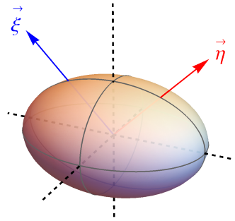
which can be easily understood from a geometric view. The $3\times 3$ real symmetric tensor $E$ possesses at least three $C_{2}$ axis (principal axis) and three symmetry plane. In order to respect the CP conserving condition in Eq. 11, $(E,\vec{\xi},\vec{\eta})$ are all invariant under the mirror reflection, therefore, $\vec{\xi}$ and $\vec{\eta}$ must lie on the same symmetry plane of $E$; see Fig. 1. The symmetric tensor $E$ can be visualized as a ellipsoid when positive definite or as a hyperboloid when not positive definite.

1) Scalar potential: Two independent CP invariants in scalar potential can be constructed from $\vec{\xi}$, $\vec{\eta}$ and $E$ [9],

$$I_{1}=(\vec{\xi}\times\vec{\eta})\cdot E\vec{\xi},\quad I_{2}=(\vec{\xi}\times\vec{\eta})\cdot E\vec{\eta}.$$

(12)

In case of $\vec{\xi}$ is collinear with $\vec{\eta}$ along direction $\vec{l}$, another invariant $(\vec{l}\times E\vec{l})\cdot E^{2}\vec{l}$ can be constructed; see Ref. [9] for details.

2) Yukawa interaction: For simplicity we consider the quark sector in this work. The Yukawa couplings for quarks in the 2HDM Lagrangian are

$\displaystyle\mathcal{L}_{\rm Yuk}=-\bar{Q}_{L}^{m}y^{mn}_{u,i}\tilde{\Phi}_{i}u^{n}_{R}-\bar{Q}_{L}^{m}y^{mn}_{d,i}\Phi_{i}d^{n}_{R}+h.c.~{},$

(13)

where $Q_{L}=(u_{L},d_{L})^{T}$ and the superscripts $m$ and $n$ sum over all generations. The Yukawa couplings $y_{u,i}$ and $y_{d,i}$ are in general complex, therefore, the Yukawa couplings $y_{1}$ and $y_{2}$ for a specific quark have four degree of freedom together. One can parameterize them by an overall strength $|\mathcal{Y}|=\sqrt{|y_{1}|^{2}+|y_{2}|^{2}}$ and three angles as

$$(y_{1},y_{2})=\mathcal{Y}(s_{\beta},c_{\beta}e^{-i\gamma})=e^{i\delta}|\mathcal{Y}|(s_{\beta},c_{\beta}e^{-i\gamma}).$$

(14)

Usually, the Yukawa coupling terms in the Lagrangian cannot be expressed in bilinear notation. One can use the bilinear notation to deal with the Yukawa couplings if the couplings can be shown to be in vector representations of $SU(2)_{\Phi}$ basis rotation. For each individual generation, $y_{u,i}$ and $y_{d,i}^{*}$ are covariant with $\Phi_{i}$ under basis transformation $\Phi_{i}\to U_{ij}\Phi_{j}$. We define covariant vectors in the dual space of $K^{\mu}$ in terms of the Yukawa couplings as follows:

$$Y_{u,\mu}\equiv y_{u,i}^{*}(\sigma_{\mu})_{ij}y_{u,j},\quad Y_{d,\mu}\equiv y_{d,i}(\sigma_{\mu})_{ij}y_{d,j}^{*},$$

(15)

which transform in the same way as $\xi_{\mu}$ and $\eta_{\mu}$, i.e.

$$(Y_{0},\vec{Y})_{u/d}^{mn}\to(Y_{0},R(U)\vec{Y})_{u/d}^{mn}.$$

(16)

The definition in Eq. 15 yields

$$\vec{Y}=|\mathcal{Y}|^{2}(s_{2\beta}c_{\gamma},-s_{2\beta}s_{\gamma},-c_{2\beta}),\quad Y_{0}=|\vec{Y}|.$$

(17)

On the other hand, the common phase of $y_{1}$ and $y_{2}$, $\delta$, is related the CKM matrix and absent in the $SO(3)_{K}$ vectors.

If the Lagrangian preserves the CP symmetry, vectors $\vec{Y}_{u/d}^{mn}$ should be invariant under the mirror reflection $\hat{\Pi}$ and lie on the same reflection plane of $\vec{\xi}$ and $\vec{\eta}$ shown in Fig. 1. We construct CP invariants as follows:

$$J_{u/d}^{mn}=(\vec{\xi}\times\vec{\eta})\cdot\vec{Y}_{u/d}^{mn}.$$

(18)

From the geometrical view, when $\vec{Y}$ is not in the same plane of $\vec{\xi}$ and $\vec{\eta}$, nonzero CP invariant $J$ is generated, and its magnitude is the “volumn” of the cross product $(\vec{\xi}\times\vec{\eta})\cdot\vec{Y}$. Considering the Yukawa interactions of $N$-generation quarks, we obtain $2N^{2}$ new CP invariants $J_{u}^{mn}$ and $J_{d}^{mn}$ where $m,n=1,2,\cdots,N$.

3) The CKM matrix: For each complex quark mass matrix $M_{u}$ and $M_{d}$, one can always perform a singular decomposition such that $V_{u}^{L}M_{u}V_{u}^{R}$ and $V_{d}^{L}M_{d}V_{d}^{R}$ are real diagonal matrices, where $V^{L,R}_{u,d}$ stands for a unitary quark basis transformation. But with three families of quarks, the complex phases in $M_{u}$ and $M_{d}$ cannot be simultaneously removed with the same $V^{L}$. Therefore, the CKM matrix $V_{\rm CKM}=(V_{u}^{L})^{\dagger}V_{d}^{L}$ [7] is left with a phase, which can be described by the so-called Jarlskog invariant [16, 17], a basis invariant quantity,

$$J=\det[M_{u}M_{u}^{\dagger},M_{d}M_{d}^{\dagger}].$$

(19)

The quark mass matrices given by Eq. 13 are $M_{u}^{mn}=y_{u,i}^{mn}v_{i}^{*}$ and $M_{d}^{mn}=y_{d,i}^{mn}v_{i}$, and each element of quark mass matrices is a $SU(2)_{\Phi}$ singlet. Since the quark masses do not exhibit any $SO(3)_{K}$ tensor structures, the Jarlskog invariant of CKM matrix constructed by $SU(3)_{L/R}$ basis rotations of quark basis is different from those CP invariants constructed by $SU(2)_{\Phi}$ rotations such as the invariants shown in Eq. 12 and Eq. 18.

To demonstrate the difference between the CP invariants in Yukawa couplings and the Jarlskog invariant in the CKM matrix explicitly, we consider the following real 2HDM potential in the Higgs basis [18],

$$H_{1}=\begin{pmatrix}G^{+}\\ \dfrac{v+\phi+iG^{0}}{\sqrt{2}}\end{pmatrix},~{}~{}~{}~{}H_{2}=\begin{pmatrix}H^{+}\\ \dfrac{R+iI}{\sqrt{2}}\end{pmatrix},$$

(20)

The potential is symmetric under the CP transformation $H_{i}\to H_{i}^{*}$:

$$V(H_{1},H_{2})=V(H_{1},H_{2})|_{H_{i}\to H_{i}^{*}},$$

(21)

demanding both $\vec{\xi}$ and $\vec{\eta}$ lie in the plane normal to $\vec{K}_{2}$, therefore $\vec{\xi}\times\vec{\eta}\propto\hat{K}_{2}$. The most general Yukawa couplings can be written as

		$\displaystyle\sum_{m,n=1}^{N}\mathcal{Y}_{u}^{mn}\bar{Q}^{m}_{L}\left(\tilde{H}_{1}\sin\beta^{mn}_{u}+e^{-i\gamma^{mn}_{u}}\tilde{H}_{2}\cos\beta^{mn}_{u}\right)u_{R}^{n}$
	$\displaystyle+$	$\displaystyle\sum_{m,n=1}^{N}\mathcal{Y}_{d}^{mn}\bar{Q}^{m}_{L}\left(H_{1}\sin\beta^{mn}_{d}+e^{i\gamma^{mn}_{d}}H_{2}\cos\beta^{mn}_{d}\right)d_{R}^{n}$
	$\displaystyle+$	$\displaystyle~{}~{}h.c.~{},$		(22)

which yields $Y_{\mu}=|\mathcal{Y}|^{2}(1,s_{2\beta}c_{\gamma},-s_{2\beta}s_{\gamma},-c_{2\beta})$ for each generation. Then CP phase in quark mass matrix is only related to the phase of overall factor $\mathcal{Y}^{mn}_{u/d}$ while CP invariants $J_{u/d}^{mn}$ are only related to $\gamma_{u/d}^{mn}$ and $\beta_{u/d}^{mn}$.

Before going further, we would like to summarize what we have learned so far. Counting the numbers of independent CP invariants in the 2HDM, there are 2 from the scalar potential, $2N^{2}$ from the Yukawa interactions, and $(N-1)(N-2)/2$ from the CKM matrix. To conserve the CP symmetry, the vectors $\vec{\xi}$, $\vec{\eta}$, and $\vec{Y}_{u/d}^{mn}$ have to lie on the same reflection plane of $E$. Each vector acts as an independent CP violation source if it departs from the reflection plane.

The effective potential of the 2HDM has been discussed extensively [21, 22, 23, 24, 25]. As a usual practice, only neutral or CP even components of Higgs boson doublets are treated as background fields, which breaks the $SU(2)_{L}$ invariance explicitly such that our previous discussions cannot apply to $V_{\rm eff}(\phi_{c})$. In order to analyze the CP property of effective potential in bilinear notation, the mass matrix needs to be evaluated in a $SU(2)_{L}$ invariant way. For that, we take all the components of the Higgs boson doublets to be background fields, and $\Phi_{i}=(\phi_{i\uparrow},\phi_{i\downarrow})^{T}$ should be understood as background fields hereafter.

1) Contributions from the scalar loop: In scenario that the scalar potential preserves the CP symmetry at the tree level, the scalar self interaction cannot induce CP violation effects in the effective potential. It sounds trivial but hitherto verified only in a specific basis. Below we provide a basis independent proof.

The mass matrices of the scalar sector cannot be analytically diagonalized, therefore we use the method in Ref. [26] to derive the bilinear form of the potential. We first expand the trace of logarithm in Eq. 24 as Taylor series and calculate the trace for each term. For example, it yields

	$\displaystyle\mathbf{Tr}(m^{2}_{S})$	$\displaystyle=8R_{\mu}A^{\mu}+4S_{\mu\nu}\eta^{\nu\mu}$
		$\displaystyle=\left(20\eta_{00}+4\operatorname{tr}(E)\right)K_{0}+24\vec{K}\cdot\vec{\eta}+8\xi_{0},$		(25)

where

	$\displaystyle S^{\mu\nu}=$	$\displaystyle R^{\mu}K^{\nu}+R^{\nu}K^{\mu}-g^{\mu\nu}(RK),$
	$\displaystyle S_{A}^{\mu\nu}=$	$\displaystyle A^{\mu}K^{\nu}+A^{\nu}K^{\mu}-g^{\mu\nu}(AK),$
	$\displaystyle A_{\mu}=$	$\displaystyle 2\eta_{\mu\nu}K^{\nu}+\xi_{\mu},$
	$\displaystyle R^{\mu}=$	$\displaystyle(1,0,0,0).$		(26)

The result is consistent with that in Ref. [27]. Our final result is

$$V_{CW}^{(S)}=\mathcal{F}\left(S^{\mu\nu}\eta_{\nu\rho},~{}S_{A}^{\mu\nu}\eta_{\nu\rho}\right),$$

(27)

where $\mathcal{F}$ is a function of the traces of $S^{\mu\nu}\eta_{\nu\rho},S_{A}^{\mu\nu}\eta_{\nu\rho}$ and their combinations [28]. If the tree level potential is invariant under the mirror reflection $\hat{\Pi}$ operation, i.e.

$$V_{\rm tree}(K_{0},\vec{K})=V_{\rm tree}(K_{0},\hat{\Pi}\vec{K}),$$

(28)

then any combination of the tensors given in Eq. CP Phases in 2HDM and Effective Potential: A Geometrical View is invariant too. As a result, the $V_{\rm CW}^{(S)}$ is also CP invariant, i.e.

$$V_{\rm CW}^{(S)}(K_{0},\vec{K})=V_{\rm CW}^{(S)}(K_{0},\hat{\Pi}\vec{K}),$$

(29)

as it should be.

2) Contributions from the gauge boson loop: The mass matrices of gauge bosons can be diagonalized and written in gauge invariant form directly. The eigenvalues of gauge boson masses obtained from the kinetic terms are

		$\displaystyle m^{2}_{Z}=\frac{g^{2}}{8}\left((1+t_{W}^{2})K_{0}+\sqrt{4t^{2}_{W}|\vec{K}|^{2}+(t_{W}^{2}-1)^{2}K_{0}^{2}}\right),$
		$\displaystyle m^{2}_{\gamma}=\frac{g^{2}}{8}\left((1+t_{W}^{2})K_{0}-\sqrt{4t^{2}_{W}|\vec{K}|^{2}+(t_{W}^{2}-1)^{2}K_{0}^{2}}\right),$
		$\displaystyle m^{2}_{W^{\pm}}=\frac{g^{2}}{4}K_{0},$		(30)

where $t_{W}=\tan\theta_{W}$, and a massless photon is ensured by the neutral vacuum condition $K_{0}=|\vec{K}|$ [8]. Therefore, the CW potential from gauge boson loop contributions $V_{\rm CW}^{(G)}=V_{\rm CW}^{(G)}(K_{0},|\vec{K}|)$ is spherically symmetric in the $K$-space,

$$V_{\rm CW}^{(G)}(K_{0},\vec{K})=V_{\rm CW}^{(G)}(K_{0},R\vec{K}),\qquad R\in O(3).$$

Furthermore, any global symmetry exhibited by the tree level potential cannot be broken by quantum corrections from gauge bosons.

3) Contributions from the quark loop: Usually, the dominant correction of quark loops to the effective potential is from the heaviest quark. Nevertheless, we include both top and bottom quarks to ensure our calculation being $SU(2)_{L}$ invariant. The top and bottom quark masses can mix as there are charged background fields. The fermion mass matrix derived from $-\partial^{2}\mathcal{L}/\partial\bar{\psi}^{i}_{L}\partial\psi^{j}_{R}$ reads as

$$(\bar{t}_{L},\bar{b}_{L})\begin{pmatrix}y_{it}\phi_{i\downarrow}^{*}&y_{ib}\phi_{i\uparrow}\\ -y_{it}\phi_{i\uparrow}^{*}&y_{ib}\phi_{i\downarrow}\end{pmatrix}\begin{pmatrix}t_{R}\\ b_{R}\end{pmatrix}.$$

(31)

After singular decomposition $M_{\rm diag}=L^{-1}MR$, two elements of the diagonalized mass matrix are

$$m_{t/b}^{2}=\dfrac{B\pm\sqrt{B^{2}+C}}{2},$$

(32)

where $B$ and $C$, in terms of $Y_{\mu}=(Y_{0},\vec{Y})$ defined in Eq. 15, are

	$\displaystyle B=$	$\displaystyle\frac{1}{2}(Y_{t0}+Y_{b0})K_{0}+\frac{1}{2}(\vec{Y}_{t}+\vec{Y}_{b})\cdot\vec{K},$
	$\displaystyle C=$	$\displaystyle-\frac{1}{2}(Y_{t}\cdot Y_{b})K_{0}^{2}-(Y_{t0}\vec{Y}_{b}+Y_{b0}\vec{Y}_{t})K_{0}\vec{K}$
		$\displaystyle+\frac{1}{2}\vec{K}\cdot(\vec{Y}_{t}\cdot\vec{Y}_{b}-Y_{t0}Y_{b0}-\vec{Y}_{t}\otimes\vec{Y}_{b}-\vec{Y}_{b}\otimes\vec{Y}_{t})\cdot\vec{K}.$

The symbol “$\otimes$” means direct product of two vectors. For illustration, we consider the special case of $y_{t}\gg y_{b}$, in which the top quark plays the leading role. The mass square of top quark is

$$m_{t}^{2}=\frac{1}{4}(Y_{t0}K_{0}+\vec{Y}_{t}\cdot\vec{K}).$$

(33)

Consider a scalar potential conserving the CP symmetry at the tree level, i.e. $V_{\rm tree}(K_{0},\vec{K})=V_{\rm tree}(K_{0},\hat{\Pi}\vec{K})$. When the Yukawa coupling breaks the CP symmetry, or equivalently, $\vec{Y}_{t/b}\neq\hat{\Pi}\vec{Y}_{t/b}$, $m_{t}^{2}$ is no longer invariant under the mirror reflection and introduces the CP violation effect to the effective potential at one-loop level,

$$V_{\rm CW}^{(F)}(K_{0},\vec{K})\neq V_{\rm CW}^{(F)}(K_{0},\hat{\Pi}\vec{K}).$$

(34)

The CP violation effect is related to $|J_{t}|$.

4) Contributions from the CKM matrix: Last but not least, we consider the impact of the Jarlskog invariant on the effective potential. Ref. [29] studied the possibility of the Jarlskog invariant entering the effective potential at three loop level, but their calculation of three-loop tadpole diagrams of the CP-odd scalar field shows no impact from the Jarlskog invariant. We notice that the CP violation effect appears in the effective potential only in the form of $SO(3)_{K}$ tensors. As the Jarlskog invariant cannot be described by the tensor structure of $SO(3)_{K}$ group, we conjecture that the CP phase in the CKM matrix would not leak into the effective potential through quantum corrections.

Without loss of generality, consider a CP-conserving Type-I 2HDM in which the $SO(3)_{K}$ covariant parameter tensors are $E$, $\vec{\xi}$, $\vec{\eta}$ and $\vec{Y}$. To respect the CP symmetry, all the tensors are invariant under a mirror symmetry $\hat{\Pi}$, i.e.

	$\displaystyle E_{ab}$	$\displaystyle=E_{cd}\Pi_{ac}\Pi_{bd},$	$\displaystyle\xi_{a}=\xi_{c}\Pi_{ac},$
	$\displaystyle\eta_{a}$	$\displaystyle=\eta_{c}\Pi_{ac},$	$\displaystyle Y_{a}=Y_{c}\Pi_{ac}.$		(35)

Any global $SU(2)_{L}$ invariant effective potential can be written as

		$\displaystyle V_{\rm eff}(\Phi_{i}^{\dagger}\Phi_{j})=V_{\rm eff}(K_{0},\vec{K})$
	$\displaystyle=$	$\displaystyle V_{\rm eff}(K_{0},T^{(1)}_{a}K_{a},T^{(2)}_{ab}K_{a}K_{b},T^{(3)}_{abc}K_{a}K_{b}K_{c},\cdots),$		(36)

where $T^{(q)}_{a_{1}\cdots a_{q}}$ transforms as a rank-$q$ tensor under the $SO(3)_{K}$ rotation. In the $K$-space the tensor $T^{(q)}_{a_{1}\cdots a_{q}}$ can be constructed by tensor products of tree level parameter tensors. Moreover, the tensor constructed by $E,\vec{\eta},\vec{\xi},\vec{Y}$ is also invariant under the mirror reflection,

$$T^{(q)}_{a_{1}\cdots a_{q}}=T^{(q)}_{b_{1}\cdots b_{q}}\Pi_{a_{1}b_{1}}\cdots\Pi_{a_{q}b_{q}}.$$

(37)

It guarantees the CP invariance of effective potential,

$$V_{\rm eff}(K_{0},\vec{K})=V_{\rm eff}(K_{0},\hat{\Pi}\vec{K}).$$

(38)

Even though the quark mass matrix, whose elements are $SU(2)_{\Phi}$ singlets, may enter $T^{(q)}_{a_{1}\cdots a_{q}}$ as a factor, tensor structures of $T^{(q)}_{a_{1}\cdots a_{q}}$ remain unchanged and the result of Eq. 38 still holds.

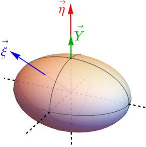
The $Z_{2}$ symmetry can be softly broken when $m_{12}^{2}\neq 0$. The vector $\vec{\eta}$ is not changed, but $\vec{\xi}=(\#,0,\#)^{T}$ points to an arbitrary direction; see Fig. 2. Hence, the scalar potential exhibits only one CP invariant, $(\vec{\xi}\times\vec{\eta})\cdot E\vec{\xi}$, and no CP invariant arises from the Yukawa interactions as $\vec{Y}\parallel\vec{\eta}$. As a result, the 2HDM potential preserving the CP symmetry at tree level still maintain the CP invariance at loop level. In addition, as shown in Eq. 43, leading thermal correction to $\vec{\xi}$, the only CP violating source, is CP conserving as both $\vec{\eta}$ and $\vec{Y}$ lie on the principal axis of $E$. As long as the length of $\vec{\eta}$ and $\vec{Y}$ are not fine tuned, $\vec{\xi}$ tends to be bend towards the principal axis at sufficient high temperatures, restoring the $Z_{2}$ and CP symmetries.

We calculated the Coleman-Weinberg potential in a basis invariant manner. The scalar potential that preserves the CP symmetry at tree level can receive CP violation corrections only from the Yukawa interactions at one-loop level. We proved that the CP phase in the CKM matrix cannot leak to effective potential at all orders based on the basis invariant form. We further showed that the leading thermal corrections shift the scalar quadratic couplings only with Yukawa and scalar quartic couplings. When a softly broken $Z_{2}$ symmetry is imposed, the scalar quadratic terms $\vec{\xi}$ is the only source that breaks $Z_{2}$ and CP symmetries, but its effect tends to be suppressed by Yukawa couplings and scalar quartic couplings at large temperature such that the $Z_{2}$ and CP symmetries tend to be restored.

References

- Lee [1973] T. D. Lee, Phys. Rev. D 8, 1226 (1973).
- Gunion and Haber [2005] J. F. Gunion and H. E. Haber, Phys. Rev. D 72, 095002 (2005), eprint hep-ph/0506227.
- Branco et al. [2005] G. C. Branco, M. N. Rebelo, and J. I. Silva-Marcos, Phys. Lett. B 614, 187 (2005), eprint hep-ph/0502118.
- Branco et al. [2012] G. C. Branco, P. M. Ferreira, L. Lavoura, M. N. Rebelo, M. Sher, and J. P. Silva, Phys. Rept. 516, 1 (2012), eprint 1106.0034.
- Battye et al. [2011] R. A. Battye, G. D. Brawn, and A. Pilaftsis, JHEP 08, 020 (2011), eprint 1106.3482.
- Pilaftsis [2012] A. Pilaftsis, Phys. Lett. B 706, 465 (2012), eprint 1109.3787.
- Kobayashi and Maskawa [1973] M. Kobayashi and T. Maskawa, Prog. Theor. Phys. 49, 652 (1973).
- Maniatis et al. [2006] M. Maniatis, A. von Manteuffel, O. Nachtmann, and F. Nagel, Eur. Phys. J. C 48, 805 (2006), eprint hep-ph/0605184.
- Maniatis et al. [2008] M. Maniatis, A. von Manteuffel, and O. Nachtmann, Eur. Phys. J. C 57, 719 (2008), eprint 0707.3344.
- Ivanov [2007] I. P. Ivanov, Phys. Rev. D 75, 035001 (2007), [Erratum: Phys.Rev.D 76, 039902 (2007)], eprint hep-ph/0609018.
- Ivanov [2008] I. P. Ivanov, Phys. Rev. D 77, 015017 (2008), eprint 0710.3490.
- Nishi [2006] C. C. Nishi, Phys. Rev. D 74, 036003 (2006), [Erratum: Phys.Rev.D 76, 119901 (2007)], eprint hep-ph/0605153.
- Botella and Silva [1995] F. J. Botella and J. P. Silva, Phys. Rev. D 51, 3870 (1995), eprint hep-ph/9411288.
- Davidson and Haber [2005] S. Davidson and H. E. Haber, Phys. Rev. D 72, 035004 (2005), [Erratum: Phys.Rev.D 72, 099902 (2005)], eprint hep-ph/0504050.
- Trautner [2019] A. Trautner, JHEP 05, 208 (2019), eprint 1812.02614.
- Jarlskog [1985] C. Jarlskog, Phys. Rev. Lett. 55, 1039 (1985).
- Dunietz et al. [1985] I. Dunietz, O. W. Greenberg, and D.-d. Wu, Phys. Rev. Lett. 55, 2935 (1985).
- Lavoura and Silva [1994] L. Lavoura and J. P. Silva, Phys. Rev. D 50, 4619 (1994), eprint hep-ph/9404276.
- Quiros [1999] M. Quiros, in ICTP Summer School in High-Energy Physics and Cosmology (1999), pp. 187–259, eprint hep-ph/9901312.
- Coleman and Weinberg [1973] S. R. Coleman and E. J. Weinberg, Phys. Rev. D 7, 1888 (1973).
- Cline et al. [2011] J. M. Cline, K. Kainulainen, and M. Trott, JHEP 11, 089 (2011), eprint 1107.3559.
- Basler et al. [2020] P. Basler, M. Mühlleitner, and J. Müller, JHEP 05, 016 (2020), eprint 1912.10477.
- Basler et al. [2017] P. Basler, M. Krause, M. Muhlleitner, J. Wittbrodt, and A. Wlotzka, JHEP 02, 121 (2017), eprint 1612.04086.
- Ferreira et al. [2020] P. M. Ferreira, L. A. Morrison, and S. Profumo, JHEP 04, 125 (2020), eprint 1910.08662.
- Basler and Mühlleitner [2019] P. Basler and M. Mühlleitner, Comput. Phys. Commun. 237, 62 (2019), eprint 1803.02846.
- Degee and Ivanov [2010] A. Degee and I. P. Ivanov, Phys. Rev. D 81, 015012 (2010), eprint 0910.4492.
- Ivanov [2009] I. P. Ivanov, Acta Phys. Polon. B 40, 2789 (2009), eprint 0812.4984.
- Cao et al. [2022] Q.-H. Cao, K. Cheng, and C. Xu (2022), eprint in preparation.
- Fontes et al. [2021] D. Fontes, M. Löschner, J. C. Romão, and J. a. P. Silva, Eur. Phys. J. C 81, 541 (2021), eprint 2103.05002.
- Glashow and Weinberg [1977] S. L. Glashow and S. Weinberg, Phys. Rev. D 15, 1958 (1977).