CP asymmetries of in models with
three Higgs doublets
Abstract
Direct CP asymmetries () in the inclusive decays of and of the order of will be probed at the BELLE II experiment. In this work, three such asymmetries are studied in the context of a three-Higgs-doublet model (3HDM), and it is shown that all three can be as large as the current experimental limits. Of particular interest is for , which is predicted to be effectively zero in the Standard Model (SM). A measurement of or more for this observable with the full BELLE II data would give evidence for physics beyond the SM. We display parameter space in the 3HDM for which such a clear signal is possible.
I Introduction
A new particle with a mass of around 125 GeV was discovered by the ATLAS and CMS collaborations of the Large Hadron Collider (LHC) Aad:2012tfa ; Chatrchyan:2012xdj . At present, the measurements of its properties are in very good agreement (within experimental error) with those of the Higgs boson of the Standard Model (SM), and hence the simplest interpretation is that the 125 GeV scalar boson is the (lone) Higgs boson of the SM (). However, an alternative possibility is that it is the first scalar to be discovered from a non-minimal Higgs sector, which contains additional scalar isospin doublets or higher representations (e.g. scalar isospin triplets). This scenario will be probed by more precise future measurements of its branching ratios (BRs), which might eventually show deviations from those of the SM Higgs boson. There would also be the possibility of discovering additional electrically neutral scalars ( or ) and/or electrically charged scalars (), and such searches form an active part of the LHC experimental programme. In the context of a two-Higgs-doublet model (2HDM) the lack of direct observation of an at the LHC together with precise measurements of SM processes exclude parameter space of (which is present in the Yukawa couplings) and (mass of the ), where , and and are the vacuum expectation values (VEVs) of the two Higgs doublets, respectively (for reviews see e.g. Branco:2011iw ,Akeroyd:2016ymd ).
In a three-Higgs-doublet model (3HDM) the Yukawa couplings of the two charged scalars depend on the four free parameters (, , , and ) of a unitary matrix that rotates the charged scalar fields in the weak eigenbasis to the physical charged scalar fields Weinberg:1976hu . The phenomenology of the lightest in a 3HDM Grossman ; Akeroyd:1994ga ; Akeroyd2 can be different to that of in a 2HDM due to the larger number of parameters that determine its fermionic couplings.
The decay , whose BR has been measured to be in good agreement with that of the SM, provides strong constraints on the parameter space of charged scalars in 2HDMs and 3HDMs. In the well-studied 2HDM Type II the bound GeV Misiak:2015xwa can be obtained and is valid for all . More precise measurements of BR at the ongoing BELLE II experiment will sharpen these constraints, but it is very unlikely that measurements of BR alone could provide evidence for the existence of an . However, the direct CP asymmetry in will be probed at the 1% level, and can be enhanced significantly above the SM prediction by additional complex phases that are present in models of physics beyond the SM Kagan:1998bh . In the context of 3HDMs we study the magnitude of three different direct CP asymmetries that involve , including the contribution of both charged scalars for the first time. We display parameter space in 3HDMs that would give a clear signal for these three observables at the BELLE II experiment.
This work is organised as follows. In section II the measurements of are summarised and the CP asymmetries in this decay are described. In section III the contribution of the charged scalars in a 3HDM to the partial decay width of is presented. Section IV contains our results, and conclusions are given in section V.
II Direct CP asymmetries in and
In this section the experimental measurements of the inclusive decays and (charged conjugated processes are implied) are described, followed by a discussion of direct CP asymmetries in these decays. The symbol signifies or (which contain anti- quarks), while signifies or (which contain quarks). The symbol denotes any hadronic final state that originates from a strange quark hadronising (e.g. states with at least one kaon), means any hadronic final state that originates from a down quark hadronising (e.g. states with at least one pion), and denotes any hadronic final state that is or .
II.1 Experimental measurements of and
There are two ways to measure the BR of the inclusive decays :
i) The fully inclusive method;
ii) The sum-of-exclusives method (also known as ”semi-inclusive”).
In the fully inclusive approach only a photon from the signal (or ) meson in the event, which decays via , is selected. Consequently, this method cannot distinguish between hadronic states and , and what is measured is actually the sum of and . From the other (or ) meson (”tag meson”) either a lepton ( or ) can be selected or full reconstruction (either hadronic or semi-leptonic) can be carried out. The former method has a higher signal efficiency, but the latter method has greater background suppression. Measurements of using the fully inclusive method with leptonic tagging have been carried out by the CLEO collaboration Chen:2001fja , the BABAR collaboration Lees:2012ufa and the BELLE collaboration Belle:2016ufb . A measurement of using the fully inclusive method with full (hadronic) reconstruction of the tag meson has so far only been carried out by the BABAR collaboration Aubert:2007my . At the current integrated luminosities (0.5 to 1 ab-1) the errors associated with measurements that involve full reconstruction are significantly larger than the errors from measurements with leptonic tagging. However, with the larger integrated luminosity at BELLE II (50 ab-1) it is expected that both approaches will provide roughly similar errors. To obtain a measurement of alone, the contribution of (which is smaller by roughly in the SM, which has also been confirmed experimentally) is subtracted.
In the sum-of-exclusives approach the selection criteria are sensitive to as many exclusive decays as possible in the hadronic final states and of the signal , as well as requiring a photon from . In contrast to the fully inclusive approach, no selection is made on the other meson in the event. The sum-of-exclusives method is sensitive to whether the decay or occurred and so this approach measures or . It has different systematic uncertainties to that of the fully inclusive approach. Measurements of have been carried out by the BABAR collaboration Lees:2012wg and the BELLE collaboration Saito:2014das . Currently, 38 exclusive decays in (about 70% of the total BR) and 7 exclusive decays in delAmoSanchez:2010ae are included. At current integrated luminosities the error in the measurement of is about twice that of the fully inclusive approach, whereas at BELLE II integrated luminosities the latter is still expected to give the more precise measurement.
Measurements in both the above approaches are made with a lower cut-off on the photon energy in the range 1.7 GeV to 2.0 GeV, and then an extrapolation is made to GeV using theoretical models. The current world average for the above six measurements of is Amhis:2019ckw :
| (1) |
The error is currently , and is expected to be reduced to around with the final integrated luminosity at the BELLE II experiment Kou:2018nap .
The theoretical prediction including corrections to order (i.e. Next-to-Next-to leading order, NNLO) is Misiak:2020vlo :
There is excellent agreement between the world average and the NNLO prediction in the SM. Consequently, allows stringent lower limits to be derived on the mass of new particles, most notably the mass of the charged scalar ( GeV Misiak:2015xwa , as mentioned earlier) in the 2HDM (Type II).
II.2 Direct CP asymmetries of and
Although it is clear that measurements of BR alone will not provide evidence for new physics with BELLE II data, the direct CP asymmetry in this decay might Kagan:1998bh . Direct CP asymmetries in and are defined as follows:
| (2) |
If is (and so ) in the definition of then the CP asymmetry is for the charged mesons, is labelled as or , and can be individually probed in a search that reconstructs or (sum-of-exclusives method). If is the CP asymmetry is for the neutral mesons, is labelled as or , and can also be individually probed. A general formula for the short-distance contribution (from ”direct photons”) to in terms of Wilson coefficients was derived in Ref. Kagan:1998bh . Prior to the publication of Ref. Kagan:1998bh a few works Wolfenstein:1994jw ; Asatrian:1996as ; Borzumati:1998tg had calculated in the SM and in specific extensions of the it that include a charged Higgs boson. The formula for in Ref. Kagan:1998bh was the first complete calculation of the asymmetry in terms of all the contributing Wilson coefficients, and was extended twelve years later to include the long-distance contributions (from ”resolved photons”) in Ref. Benzke:2010tq . In approximate form is as follows:
| (3) | |||||
The above four asymmetries are obtained from eq. (3) with the choices for (the charge of the spectator quark) and given in Tab. 1.
The parameters are hadronic parameters that determine the magnitude of the long-distance contribution. Their allowed ranges were updated in Ref. Gunawardana:2019gep to be as follows:
| (4) |
The short-distance contributions to are the terms that are independent of , and if long-distance terms are neglected. Other parameters are as follows: , (in terms of Wolfenstein parameters), . The ’s are Wilson coefficients of relevant operators that are listed in Ref. Kagan:1998bh . In the SM the Wilson coefficients are real and the only term in that is non-zero is the term with . Due to being of order while is of order 1, for the imaginary parts one has . For the short-distance contribution only (i.e. neglecting the term with in eq. (3)) one has and . The small value of in the SM suggests that this observable could probe models of physics beyond the SM that contain Wilson coefficients with an imaginary part.
After the publication of Ref. Kagan:1998bh , several works calculated (for the short-distance contribution only) in the context of specific models of physics beyond the SM Chua:1998dx , usually in supersymmetric extensions of it. Values of of up to were shown to be possible in specific models, while complying with stringent constraints from electric dipole moments (EDMs). Including the long-distance contributions, it was shown in Ref. Benzke:2010tq that the the SM prediction using eq. (3) is enlarged to the range , and (using updated estimates of the parameters) is further increased to in Ref. Gunawardana:2019gep . This revised SM prediction has decreased the effectiveness of as a probe of physics beyond the SM. Consequently, in Ref. Benzke:2010tq the difference of CP asymmetries for the charged and neutral mesons was proposed, which is given by:
| (5) |
This formula is obtained from eq. (3) in which only the terms with do not cancel out. The SM prediction is (due to the the Wilson coefficients being real) and hence this observable is potentially a more effective probe of new physics than . Note that depends on the product of a long-distance term (, whose value is only known to within an order of magnitude) and two short-distance terms ( and ).
An alternative observable is the untagged (fully inclusive) asymmetry given by
| (6) |
Here is the ratio . The parameter is defined as the following ratio:
| (7) |
where is the number of mesons that decay to etc. Experimentally, Kou:2018nap and in our numerical analysis we take . In the fully inclusive measurement of BR() the asymmetry is measured by counting the difference in the number of positively and negatively charged leptons from the tagged (not signal) meson. The SM prediction of is essentially 0 Soares:1991te ; Kagan:1998bh (up to tiny corrections), even with the long-distance contribution included. Hence this observable is a cleaner test of new physics than . The first studies of the magnitude of the untagged asymmetry in the context of physics beyond the SM were in Ref. Akeroyd:2001cy , and the importance of this observable was emphasised in Ref. Hurth:2003dk . In this work we will consider the above three direct CP asymmetries in the context of 3HDMs: i) , ii) , iii) .
Measurements of all three asymmetries have been carried out, and the most recent BELLE and BABAR measurements are summarised in Tab. 2. In Tab. 2 the CP asymmetry would have the same magnitude as the average if the production cross-sections of and were the same. The BELLE measurement Watanuki:2018xxg of differs only slightly from the BELLE measurement of in Tab. 2. The world averages are taken from Ref. Tanabashi:2018oca . The given averages for and are obtained from the two displayed measurements in Tab. 2, while the average for also includes two earlier BABAR measurements and the CLEO measurement Coan:2000pu .
| BELLE | BABAR | World Average | |
|---|---|---|---|
| Watanuki:2018xxg | Lees:2014uoa | Tanabashi:2018oca | |
| Pesantez:2015fza | Lees:2012ufa | Tanabashi:2018oca | |
| Watanuki:2018xxg | Lees:2014uoa | Tanabashi:2018oca |
At BELLE II all three asymmetries will be measured with greater precision Kou:2018nap . At present around 74 fb-1 of integrated luminosity have been accumulated, which is about one tenth of the integrated luminosity at the BELLE experiment, and about one sixth that at the BABAR experiment. By the end of the year 2021 about 1 ab-1 is expected, and thus measurements of at BELLE II will then match (or better) in precision those at BELLE and BABAR. For an integrated luminosity of 50 ab-1 (which is expected to be obtained by the end of the BELLE II experiment in around the year 2030), the estimated precision for is 0.19%, for is (leptonic tag) and (hadronic tag), and for is 0.3% (sum-of-exclusives) and 1.3% (fully inclusive with hadronic tag, and so it measures a sum of and ). These numbers are summarised in Tab. 3, together with the SM predictions. Due to the SM prediction of being essentially zero, a central value of 2.5% with 0.5% error would constitute a signal of physics beyond the SM. For , whose prediction in the SM is also essentially zero, a central value of 1.5% with 0.3% error would constitute a signal. Note that the current allowed range of is ( at ). Comparing this range with the SM prediction of shows that it is less likely that the observable alone could provide a clear signal of physics beyond the SM, e.g. a future central value of above (which is outside the current range) with the expected of error 0.19% would be required to give a discrepancy from the upper SM prediction of 3.3%.
| SM Prediction | Leptonic tag | Hadronic tag | Sum of exclusives | |
|---|---|---|---|---|
| x | x | 0.19% | ||
| 0 | 0.48% | 0.70% | x | |
| 0 | x | 1.3% | 0.3% |
III The decays and in the 3HDM
In this section the theoretical structure of the 3HDM is briefly introduced, followed by a discussion of the Wilson coefficients. Finally, the expressions for the BRs of and are given.
III.1 Fermionic couplings of the charged scalars in a 3HDM
In a 3HDM, two isospin scalar doublets (with hypercharge ) are added to the Lagrangian of the SM. There are two (physical) charged scalars and for a more detailed description of the model we refer the reader to Refs. Cree:2011uy ; Akeroyd:2019mvt . In order to eliminate tree-level flavour changing neutral currents (FCNCs) that are mediated by scalars, the couplings of the scalar doublets to fermions (”Yukawa couplings”) are assumed to be invariant under certain discrete symmetries (a requirement called ”natural flavour conservation” (NFC), e.g. see Refs. Glashow:1976nt ; Branco:2011iw ). The Lagrangian that describes the interactions of and (the two charged scalars of the 3HDM, which we do not order in mass) with the fermions is given as follows:
| (8) |
Here refers to the up(down)-type quarks, and refers to the electron, muon and tau. In a 2HDM there is only one charged scalar, and the parameters , , and (with no subscript) are equal to or (where , the ratio of vacuum expectation values). In contrast, in a 3HDM the , , and () each depend on four parameters of a unitary matrix , and thus the phenomenology of and can differ from that of in a 2HDM. This matrix connects the charged scalar fields in the weak eigenbasis ( with the physical scalar fields (, ) and the charged Goldstone boson as follows:
| (9) |
The couplings , and in terms of the elements of are Cree:2011uy :
| (10) |
and
| (11) |
The values of , , and in these matrix elements are given in Tab. 4 and depend on which of the five distinct 3HDMs is being considered. The choice of , , and indicates that the down-type quarks receive their mass from , the up-type quarks from , and the charged leptons from (and is called the “Democratic 3HDM”). The other possible choices of , , and in a 3HDM are given the same names as the four types of 2HDM.
| 3HDM (Type I) | 2 | 2 | 2 |
| 3HDM (Type II) | 2 | 1 | 1 |
| 3HDM (Lepton-specific) | 2 | 2 | 1 |
| 3HDM (Flipped) | 2 | 1 | 2 |
| 3HDM (Democratic) | 2 | 1 | 3 |
The elements of the matrix can be parametrised by four parameters , , , and , where
| (12) |
The angle and phase can be written explicitly as functions of several parameters in the scalar potential Cree:2011uy . The explicit form of is:
| (25) | |||||
| (29) |
Here and denote the sine or cosine of the respective angle. Hence the functional forms of , , and in a 3HDM depend on four parameters. As mentioned earlier, this is in contrast to the analogous couplings in the 2HDM for which is the only free coupling parameter.
The parameters , and are constrained (for a specific value of ) by direct searches for (e.g. at the LHC) and by their effect on low-energy observables in flavour physics. A summary of these constraints can be found in Ref. Cree:2011uy , in which the lightest charged scalar is assumed to give the dominant contribution to the observable being considered. A full study in the context of the 3HDM with both charged scalars contributing significantly has not been performed, and is beyond the scope of this work. The coupling is most strongly constrained from the process from LEP data. For around 100 GeV the constraint is roughly (assuming , so that the dominant contribution is from the coupling), and weakens with increasing mass of the charged scalar. Constraints on the and are weaker and we take and as being representative of these constraints for around 100 GeV.
The couplings do not enter the partial width of , and only the couplings to quarks are relevant ( and ). Consequently, the partial width for in Type I and the lepton-specific structures (which have identical functional forms for and due to in Tab. 4) has the same dependence on the parameters of . Likewise, the partial width for in Type II, flipped and democratic structures ( in Tab. 4) is the same. The contribution of and to BR() has been studied in the 3HDM at the leading order (LO) in Ref. Hewett:1994bd (no corrections arising from diagrams with charged scalars) and at next-to-leading order (NLO) in Ref. Akeroyd:2016ssd ( corrections arising from diagrams with charged scalars). In Ref. Akeroyd:2016ssd the effect of a non-zero phase was not studied, and direct CP asymmetries were not considered. Previous studies of (and ), but not and , in models with one charged scalar (e.g. 2HDM, or the lightest of a 3HDM or multi-Higgs doublet model) have been carried out in Refs. Wolfenstein:1994jw ; Asatrian:1996as ; Borzumati:1998tg ; Kiers:2000xy ; Jung:2010ab ; Jung:2012vu .
III.2 Wilson coefficients in 3HDM
The direct CP asymmetry given by eq. (3) is written in terms of Wilson coefficients, which (for observables) are generally evaluated at the scale of . We use the explicit formulae in Ref. Borzumati:1998tg for the Wilson coefficients at LO and NLO in the 2HDM, and apply them to the 3HDM (generalising the expressions to account for the two charged scalars). The LO Wilson coefficients Hewett:1994bd at the matching scale are as follows:
| (30) | ||||
| (31) | ||||
| (32) | ||||
| (33) |
Terms with , , and are absent because (as is usually taken) in the effective Hamiltonian. Explicit forms for all and are given in Ref. Borzumati:1998tg : those for the SM contribution are functions of while those for and are functions of and , respectively.
The NLO Wilson coefficients at the matching scale are as follows:
| (34) | ||||
| (35) | ||||
| (36) | ||||
| (37) | ||||
| (38) |
Explicit forms for all functions are given in Ref. Borzumati:1998tg . Renormalisation group running is used to evaluate the Wilson coefficients at the scale .
The partial width for has four distinct parts: i) Short-distance contribution from the partonic process (to a given order in perturbation theory); ii) Short-distance contribution from the partonic process; iii) and iv) Non-perturbative corrections that scale as and , respectively. The partial width of is as follows:
| (39) | |||||
The short-distance contribution is contained in , with given by:
| (40) |
The Wilson coefficient is a linear combination of , and , while is a linear combination of these three LO coefficients as well as the NLO coefficients , , , and . The parameter is a summation over all the LO Wilson coefficients which are evaluated at the scale . The contribution from is contained in , and the remaining two terms are the non-perturbative contributions. In there are terms of order , but to only keep terms to the NLO order for a consistent calculation (to ) the following form is used in Ref. Borzumati:1998tg :
| (41) |
| (42) |
The dependence is removed by using the measured value of the semi-leptonic branching ratio and its partial width (which also depends on ), and BR can be written as follows:
| (43) |
IV Numerical results
The four input parameters that determine , , and are varied in the following ranges, while respecting the constraints , and for GeV.
| (44) |
As mentioned in section III.A, the functional dependence on these four input parameters of the observables BR, , and is the same in the Flipped 3HDM, Type II and Democratic 3HDMs. Results will be shown in this class of models, and sizeable values of the asymmetries are shown to be possible. Results are not shown for the Model Type I and lepton specific structures because the asymmetries in these two models do not differ much from the SM values, the reason being that the products and (which enter the Wilson coefficients) are real in these two models, leading to real and . The couplings are different functions of , , and in the Flipped 3HDM, Type II and Democratic 3HDMs, and thus the constraints in eq. (44) on rule out different regions of the four input parameters in each model. However, the constraints from are quite weak, and so the allowed parameter space from , and for GeV is essentially the same in all three models under consideration. For definiteness, our results will presented in the context of the Flipped 3HDM. In eq. (1) for the measurement of BR we take the allowed range, giving .


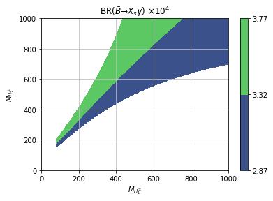


In Figs. 1a and 1b the magnitude of BR in the plane is plotted with , and . In the left panel and in the right panel . In Ref. Akeroyd:2016ssd only was taken when studying BR in 3HDMs. In our numerical analysis we set the normalisation scale to be GeV (the central value of the quark pole mass), and the uncertainty in the asymmetries due to the choice of is discussed later. It can be seen in Fig. 1a and Fig. 1b that for this choice of parameters the non-zero value of significantly increases the allowed parameter space in the plane . In Figs. 2a and 2b the parameters are taken to be , and . In the left panel and in the right panel . In this case the non-zero value of significantly decreases the parameter space in the plane , although a region with and becomes allowed for . In all these plots the notation is not used and both masses are scanned in the range 80 GeV GeV. It is clear that the phase can have a sizeable effect the parameter space of in the 3HDM.
In an earlier work by some of us Akeroyd:2018axd the region allowed by BR in the plane in the Flipped 3HDM was obtained by using the constraint only, with . This is a result from the Aligned 2HDM for small , and when applied to an of the 3HDM it is neglecting the contributions of , and . In Fig. 3a and Fig. 3b we compare this approximation with the full BR constraint in the 3HDM. In Fig. 3a, the allowed region in the plane is plotted with , 85 GeV, GeV with . The region is much smaller than that displayed in Ref. Akeroyd:2018axd , which used the constraint in the same plane; decreasing below 600 GeV leads to no allowed parameter space of for this choice of parameters. In Fig. 3b, which has , but other parameters the same as in Fig. 3a, one can see that the allowed region is much larger, and is in fact more similar in extent (although still smaller) than that allowed from the constraint with in Ref. Akeroyd:2018axd . Hence the approximate constraint does not give a very accurate exclusion of parameter space, but the inclusion of a non-zero value of can (very roughly) reproduce the allowed regions in Ref. Akeroyd:2018axd (which focussed on the possibility of a large BR) in the Flipped 3HDM with ). In Fig. 4a and Fig. 4b we take 130 GeV, GeV (i.e. a smaller mass splitting between the charged scalars) and . In Fig. 4a we take and in Fig. 4b . One can see that for very little parameter space is allowed by BR. In contrast, for a sizeable region of the plane is permitted. We calculated BR) in the same plane but with and found that is essentially the same as the case with in Ref. Akeroyd:2018axd . Hence there is a sizeable parameter space for a large BR) in the Flipped 3HDM while satisfying the full BR constraint, provided that is non-zero.
We now turn our attention to the CP asymmetries. For we use , which is obtained by taking . The CP asymmetries are evaluated at , so that we use the LO formulae for the Wilson coefficients , , and in eq. (3). In order to evaluate the CP asymmetries at , it is necessary to include not only the NLO terms of these Wilson coefficients but also the NNLO terms of and .
In Fig. 5a, Fig. 5b, and Fig. 6 the asymmetries , , and are (respectively) plotted in the plane . In all these figures the remaining four 3HDM parameters are fixed as GeV, GeV, and , whereas the long-distance (hadronic) parameters are taken to be GeV, GeV and GeV.


The scale is taken to be 4.77 GeV (pole mass ). The three red lines (from left to right) show the upper () limit, the central value, and the lower () limit for BR. The white region in Fig.5a with roughly violates the current experimental () limit for (the white regions in Figs.5a, 5b and 6 with correspond to parameter choices not covered in the scan). In Fig. 5a, in the parameter space allowed by BR the magnitude of is roughly between and , which is within the current experimental limits. In Fig. 5b, can reach , which would provide a signal at BELLE II with 50 ab-1. We note that is directly proportional to , which has been taken to have its largest allowed value. If is reduced then will decrease proportionally. In Fig.6 it is shown that can reach almost , which would be a signal at BELLE II. The parameter has a subdominant effect on (in contrast to ) and so is possible, independent of the value of . We note that there is more parameter space in a 3HDM for such large asymmetries than in the Aligned 2HDM Jung:2010ab ; Jung:2012vu . This is because there is more possibility for cancellation in the contributions of and to (while having a large asymmetry), but in the Aligned 2HDM there is only one charged scalar and no and coupling.


In Figs. 7a, 7b, and 8 the contours of the CP asymmetries are shown in the plane . The other parameters are fixed as GeV, GeV, , and . The scale and the hadronic parameters are taken to be the same as in Figs. 5a, 5b and 6. Inside the red circles the predicted BR satisfies the current () experimental constraint, and restricts the allowed parameter space to be roughly and (i.e. an ellipse centred on around ). The white regions in all plots violate the current experimental limits (see Table II) on the displayed asymmetry. In Fig. 7a it can be seen that roughly the right half () of the ellipse is ruled out from . In Figs. 7b and 8, in the allowed region of the plane the asymmetries increase in magnitude as is varied from to , and values of and can again be reached. The theoretical uncertainty is significant, and will be quantified in what follows.
We now consider the theoretical uncertainty of our predictions that arise from varying the scale and the hadronic parameters. In Tabs. V, VI and VII the parameters are fixed as GeV, GeV, and (same as in Figs. 5a, 5b and 6); and (same as in Figs. 7a, 7b and 8). Tab. V uses the lowest possible values of the hadronic parameters, Tab. VI uses the central values, and Tab. VII uses the maximum values. In each table the value of the scale is taken to be , and . The pole quark mass is GeV, and in Tabs.V, VI and VII we take 4.71 GeV, 4.77 GeV and 4.83 GeV respectively. This scale dependence corresponds to the NNLO contributions in BR and the NLO contributions in the CP asymmetries. The uncertainty from is around 50 % for and in each table. One can see that increasing the scale makes both and more negative. The CP asymmetry is very significantly affected by the change of the hadronic parameters, so that even the sign of the asymmetry is flipped. The effect of the change of the hadronic parameters on is also severe (due to it being proportional to ), while the effect on is less significant. The maximum and minimum values of the observables in Tabs. V, VI and VII are as follows:
| (45) | |||
| (46) | |||
| (47) | |||
| (48) |
We note that a full scan over the hadronic parameters might result in larger asymmetries.
| % | % | % | ||
|---|---|---|---|---|
| % | % | % | ||
|---|---|---|---|---|
| % | % | |||
|---|---|---|---|---|
IV.1 Electric dipole moments, collider limits and theoretical consistency
In a separate publication EDMs , some of us addressed the calculation of both the neutron and EDMs in the 3HDM discussed here, as these observables will be affected by a non-zero value of the CP violating (CPV) phase . Without pre-empting the results to appear therein, it has been checked that the regions of 3HDM parameter space explored in our present analysis are generally compliant with constraints coming from both neutron and electron EDMs. However, some regions of the parameter space covered here would be excluded. Specifically, with reference to the and values adopted and the plane considered, we can anticipate that the regions centred around and and 4.6 would be excluded by the combination of the two EDMs. However, the expanse of such an invalid parameter space diminshes significantly as and get closer, to the extent that no limits can be extracted from such observables in the case of exact mass degeneracy of the two charged Higgs states, for suitable values of their Yukawa couplings. Hence, the majority of the results presented here are stable against EDM constraints. Indeed, it should further be noted that both in the present paper and in Ref. EDMs , for computational reasons, the neutral Higgs sector of the 3HDM has essentially been decoupled. Hence, in the case of a lighter neutral scalar spectrum one may potentially invoke cancellations occurring between the charged and neutral Higgs boson states (including the SM-like one) of the CPV 3HDM (in the same spirit as those of Ref. Kanemura:2020ibp for the CPV Aligned 2HDM), which could further reduce the impact of EDM constraints. Moreover, one also ought to make sure that the and spectra of masses and couplings adopted here do not violate bounds coming from colliders, specifically LEP/SLC, Tevatron and the LHC. Again, based on the forthcoming results of Ref. EDMs , we anticipate this being the case in the present context. Finally, in Ref. EDMs , it will also be shown that the values of the Yukawa parameters adopted in this paper are compliant with theoretical self-consistency requirements of the 3HDM stemming from vacuum stability and perturbativity.
V Conclusions
In the context of 3HDMs with NFC the magnitudes of three CP asymmetries that involve the decay have been studied. In the SM, the CP asymmetry in the inclusive decay alone () has a theoretical error from long-distance contributions that render it unlikely to provide a clear signal of physics beyond the SM at the ongoing BELLE II experiment. The untagged asymmetry () and the difference of CP asymmetries () are both predicted to be essentially zero in the SM, with negligible theoretical error. Hence these latter two observables offer better prospects of revealing new physics contributions to .
In the context of 3HDMs there are two charged scalars that contribute to the process . There are six new physics parameters (two masses of the charged scalars, and four parameters that determine the Yukawa couplings of the charged scalars) that together enable the relevant Wilson coefficients to contain a sizeable imaginary part. In three of the five types of 3HDM the magnitude of and can reach values such that a signal at the BELLE II experiment with 50 ab-1 of integrated luminosity would be possible. Although the parameter space for such a clear signal is rather small (which is also usually the case in other models of physics beyond the SM), it was shown that a 3HDM could accommodate any such signal, and thus would be a candidate model for a statistically significant excess (beyond the SM prediction) in these asymmetry observables.
Acknowledgements
AA and SM are supported in part through the STFC Consolidated Grant ST/L000296/1. SM is supported in part through the NExT Institute. SM and MS acknowledge the H2020-MSCA-RISE-2014 grant no. 645722 (NonMinimalHiggs). TS is supported in part by JSPS KAKENHI Grant Number 20H00160. TS and SM are partially supported by the Kogakuin University Grant for the project research ”Phenomenological study of new physics models with extended Higgs sector”. We thank H. E. Logan and D. Rojas-Ciofalo for reading the manuscript and for useful comments.
References
- (1) G. Aad et al. [ATLAS Collaboration], Phys. Lett. B 716, 1 (2012) [arXiv:1207.7214 [hep-ex]].
- (2) S. Chatrchyan et al. [CMS Collaboration], Phys. Lett. B 716, 30 (2012) [arXiv:1207.7235 [hep-ex]].
- (3) G. C. Branco, P. M. Ferreira, L. Lavoura, M. N. Rebelo, M. Sher and J. P. Silva, Phys. Rept. 516, 1-102 (2012) [arXiv:1106.0034 [hep-ph]].
- (4) A. G. Akeroyd et al., Eur. Phys. J. C 77, no. 5, 276 (2017) [arXiv:1607.01320 [hep-ph]].
- (5) S. Weinberg, Phys. Rev. Lett. 37, 657 (1976); C. H. Albright, J. Smith and S. H. H. Tye, Phys. Rev. D 21, 711 (1980); G. C. Branco, A. J. Buras and J. M. Gerard, Nucl. Phys. B 259, 306 (1985).
- (6) Y. Grossman, Nucl. Phys. B 426, 355 (1994) [hep-ph/9401311].
- (7) A. G. Akeroyd and W. J. Stirling, Nucl. Phys. B 447, 3 (1995).
- (8) A. G. Akeroyd, S. Moretti and J. Hernandez-Sanchez, Phys. Rev. D 85, 115002 (2012) [arXiv:1203.5769 [hep-ph]].
- (9) M. Misiak, H. M. Asatrian, R. Boughezal, M. Czakon, T. Ewerth, A. Ferroglia, P. Fiedler, P. Gambino, C. Greub, U. Haisch, T. Huber, M. Kaminski, G. Ossola, M. Poradzinski, A. Rehman, T. Schutzmeier, M. Steinhauser and J. Virto, Phys. Rev. Lett. 114, no.22, 221801 (2015) [arXiv:1503.01789 [hep-ph]].
- (10) A. L. Kagan and M. Neubert, Phys. Rev. D 58, 094012 (1998) [arXiv:hep-ph/9803368 [hep-ph]].
- (11) S. Chen et al. [CLEO], Phys. Rev. Lett. 87, 251807 (2001) [arXiv:hep-ex/0108032 [hep-ex]].
- (12) J. P. Lees et al. [BaBar], Phys. Rev. D 86, 112008 (2012) [arXiv:1207.5772 [hep-ex]]; J. P. Lees et al. [BaBar], Phys. Rev. Lett. 109, 191801 (2012) [arXiv:1207.2690 [hep-ex]].
- (13) A. Abdesselam et al. [Belle], [arXiv:1608.02344 [hep-ex]].
- (14) B. Aubert et al. [BaBar], Phys. Rev. D 77, 051103 (2008) [arXiv:0711.4889 [hep-ex]].
- (15) J. P. Lees et al. [BaBar], Phys. Rev. D 86, 052012 (2012) [arXiv:1207.2520 [hep-ex]].
- (16) T. Saito et al. [Belle], Phys. Rev. D 91, no.5, 052004 (2015) [arXiv:1411.7198 [hep-ex]].
- (17) P. del Amo Sanchez et al. [BaBar], Phys. Rev. D 82, 051101 (2010) [arXiv:1005.4087 [hep-ex]].
- (18) Y. S. Amhis et al. [HFLAV], [arXiv:1909.12524 [hep-ex]].
- (19) E. Kou et al. [Belle-II], PTEP 2019, no.12, 123C01 (2019) [arXiv:1808.10567 [hep-ex]].
- (20) M. Misiak, A. Rehman and M. Steinhauser, [arXiv:2002.01548 [hep-ph]].
- (21) L. Wolfenstein and Y. L. Wu, Phys. Rev. Lett. 73, 2809-2812 (1994) [arXiv:hep-ph/9410253 [hep-ph]]; Y. L. Wu, Chin. Phys. Lett. 16, 339-941 (1999) [arXiv:hep-ph/9805439 [hep-ph]].
- (22) G. M. Asatrian and A. Ioannisian, Phys. Rev. D 54, 5642-5646 (1996) [arXiv:hep-ph/9603318 [hep-ph]]; H. M. Asatrian, G. K. Egiian and A. N. Ioannisian, Phys. Lett. B 399, 303-311 (1997).
- (23) F. Borzumati and C. Greub, Phys. Rev. D 58, 074004 (1998) [arXiv:hep-ph/9802391 [hep-ph]].
- (24) M. Benzke, S. J. Lee, M. Neubert and G. Paz, Phys. Rev. Lett. 106, 141801 (2011) [arXiv:1012.3167 [hep-ph]].
- (25) A. Gunawardana and G. Paz, JHEP 11, 141 (2019) [arXiv:1908.02812 [hep-ph]].
- (26) C. K. Chua, X. G. He and W. S. Hou, Phys. Rev. D 60, 014003 (1999) [arXiv:hep-ph/9808431 [hep-ph]]; Y. G. Kim, P. Ko and J. S. Lee, Nucl. Phys. B 544, 64-88 (1999) [arXiv:hep-ph/9810336 [hep-ph]]; M. Aoki, G. C. Cho and N. Oshimo, Phys. Rev. D 60, 035004 (1999) [arXiv:hep-ph/9811251 [hep-ph]]; L. Giusti, A. Romanino and A. Strumia, Nucl. Phys. B 550, 3-31 (1999) [arXiv:hep-ph/9811386 [hep-ph]]; S. Baek and P. Ko, Phys. Rev. Lett. 83, 488-491 (1999) [arXiv:hep-ph/9812229 [hep-ph]]; T. Goto, Y. Y. Keum, T. Nihei, Y. Okada and Y. Shimizu, Phys. Lett. B 460, 333-340 (1999) [arXiv:hep-ph/9812369 [hep-ph]]; M. Aoki, G. C. Cho and N. Oshimo, Nucl. Phys. B 554, 50-66 (1999) [arXiv:hep-ph/9903385 [hep-ph]]. T. Goto, Y. Okada, Y. Shimizu, T. Shindou and M. Tanaka, Phys. Rev. D 70, 035012 (2004) [arXiv:hep-ph/0306093 [hep-ph]].
- (27) J. M. Soares, Nucl. Phys. B 367, 575-590 (1991).
- (28) A. G. Akeroyd, Y. Y. Keum and S. Recksiegel, Phys. Lett. B 507, 252-259 (2001) [arXiv:hep-ph/0103008 [hep-ph]]. A. G. Akeroyd and S. Recksiegel, Phys. Lett. B 525, 81-88 (2002) [arXiv:hep-ph/0109091 [hep-ph]].
- (29) T. Hurth, E. Lunghi and W. Porod, Nucl. Phys. B 704, 56-74 (2005) [arXiv:hep-ph/0312260 [hep-ph]].
- (30) S. Watanuki et al. [Belle], Phys. Rev. D 99, no.3, 032012 (2019) [arXiv:1807.04236 [hep-ex]].
- (31) J. P. Lees et al. [BaBar], Phys. Rev. D 90, no.9, 092001 (2014) [arXiv:1406.0534 [hep-ex]].
- (32) M. Tanabashi et al. [Particle Data Group], Phys. Rev. D 98, no.3, 030001 (2018).
- (33) L. Pesántez et al. [Belle], Phys. Rev. Lett. 114, no.15, 151601 (2015) [arXiv:1501.01702 [hep-ex]].
- (34) T. E. Coan et al. [CLEO], Phys. Rev. Lett. 86, 5661-5665 (2001) [arXiv:hep-ex/0010075 [hep-ex]].
- (35) S. L. Glashow and S. Weinberg, Phys. Rev. D 15, 1958 (1977); E. A. Paschos, Phys. Rev. D 15, 1966 (1977).
- (36) A. G. Akeroyd, S. Moretti and M. Song, Phys. Rev. D 101, no.3, 035021 (2020) [arXiv:1908.00826 [hep-ph]].
- (37) G. Cree and H. E. Logan, Phys. Rev. D 84, 055021 (2011) [arXiv:1106.4039 [hep-ph]].
- (38) S. L. Glashow and S. Weinberg, Phys. Rev. D 15, 1958 (1977); E. A. Paschos, Phys. Rev. D 15, 1966 (1977).
- (39) J. L. Hewett, [arXiv:hep-ph/9406302 [hep-ph]].
- (40) A. G. Akeroyd, S. Moretti, K. Yagyu and E. Yildirim, Int. J. Mod. Phys. A 32, no.23n24, 1750145 (2017) [arXiv:1605.05881 [hep-ph]].
- (41) K. Kiers, A. Soni and G. H. Wu, Phys. Rev. D 62, 116004 (2000) [arXiv:hep-ph/0006280 [hep-ph]].
- (42) M. Jung, A. Pich and P. Tuzon, Phys. Rev. D 83, 074011 (2011) [arXiv:1011.5154 [hep-ph]].
- (43) M. Jung, X. Q. Li and A. Pich, JHEP 10, 063 (2012) [arXiv:1208.1251 [hep-ph]].
- (44) A. G. Akeroyd, S. Moretti and M. Song, Phys. Rev. D 98, no.11, 115024 (2018) [arXiv:1810.05403 [hep-ph]].
- (45) H.E. Logan, S. Moretti, D. Rojas-Ciofalo and M. Song, in preparation.
- (46) S. Kanemura, M. Kubota and K. Yagyu, JHEP 2008, 026 (2020) [arXiv:2004.03943 [hep-ph]].