Covid-19 Analysis Using Tensor MethodsD. Dulal, R. Goudarzi Karim, and C. Navasca
Covid-19 Pandemic Data Analysis using Tensor Methods ††thanks: Submitted to the editors December 29, 2022. \fundingThis work was funded by National Science Foundation under Grant No. DMS-1439786 and Grant No. MCB-2126374.
Abstract
In this paper, we use tensor models to analyze Covid-19 pandemic data. First, we use tensor models, canonical polyadic and higher-order Tucker decompositions, to extract patterns over multiple modes. Second, we implement a tensor completion algorithm using canonical polyadic tensor decomposition to predict spatiotemporal data from multiple spatial sources and to identify Covid-19 hotspots. We apply a regularized iterative tensor completion technique with a practical regularization parameter estimator to predict the spread of Covid-19 cases and to find and identify hotspots. Our method can predict weekly and quarterly Covid-19 spreads with high accuracy. Third, we analyze Covid-19 data in the US using a novel sampling method for alternating least-squares. Moreover, we compare the algorithms with standard tensor decompositions it terms of their interpretability, visualization and cost analysis. Finally, we demonstrate the efficacy of the methods by applying the techniques to New Jersey’s Covid-19 case tensor data.
keywords:
tensor, tensor completion, tensor decomposition, Covid-19, spatio-temporal data1 Introduction
Tensor decomposition is a powerful tool in data analysis, computer vision, scientific computing, machine learning and many other fields. In fact, tensor models for dimensionality reduction have been highly effective in machine learning applications like classification and regression. Tensor decomposition on its own have been successful in many modern big data analysis [11, 8, 24, 31].
In this work, we focus on analyzing Covid-19 pandemic data [28, 1] by using tensor decomposition models. Our goals are to predict future infection, locate and identify hotspots from data-set coming from multiple sources across different spatial regions over time. One is interested in determining where and when changes occur in the pattern. The strategy is set up an optimization which separates the data in following: let where is the given tensor, is a low rank reconstructed tensor of and is the sparse tensor. In video processing, the original video is separated into its background and foreground subspace to detect anomalous activities [11, 32]. The tensor is the background, and is the foreground. The sparse tensor can provide anomalous activities. Similarly, will contain hotspot occurrence. To achieve this separation, we formulate the following:
| (1) |
where , is the tensor Frobenius norm, and is the vector one norm. The optimization problem (1) is neither convex nor differentiable [12]. In addition, this formulation is amenable to tensor completion problems where one can find missing data. This is basis for predicting future Covid-19 infection cases in presence of previous pandemic data.
Most of the algorithms suggested for solving (1) are based on ALS (alternating least squares) [12]. ALS is fast, easy to program and effective. However, ALS has some drawbacks. There is a need for more efficient and accurate methods. Thus, we propose a sampling method for ALS to leverage the efficiency of ALS and to allow bigger tensor data.
1.1 Previous Work on Covid-19 Data Analysis
Here, we mention a non-exhaustive collection of literature on Covid-19 analysis. The work varies from PDE models to machine learning methods for the prediction of Covid-19 hotspots, patterns, and outbreaks. A parabolic PDE-based predictive model with learned parameters from training data of preceding Covid-19 cases has been proposed to predict Covid-19 infections in Arizona[29]. A tensor train global optimization is used to explore the parameter space to locate the starting points, and the Nelder-Mead simplex local optimization algorithm is used for the local optimization of the covid-19 modeling problem and eventually, Runge-Kutta method was applied to solve the PDE for one step forward prediction. There are several machine learning methods. In supervised machine learning, time series forecasting via Holt’s Winter model was used to analyze global Covid-19 data and predict the sum of global Covid-19 cases in comparison to linear regression and support vector algorithms. Dictionary learning [19] through non-negative matrix factorization to identify the pattern and to predict future covid-19 outbreaks. In addition, machine learning has been applied to a susceptible-exposed-infected-removed (SEIR) model with SARS 2003 training data to predict covid-19 outbreaks [33]. Deep learning models like attention-based encoder-decoder model [20] have been implemented to forecast covid-19 outbreak. There needs to be more work on mathematical modeling to detect covid-19 hotspots; however, a tensor-based anomaly detection method for spatial-temporal data[34] has been proposed to determine hotspots based on an anomaly in pattern.
1.2 Contributions.
In this work, we focus on analyzing Covid-19 infection data [28, 1] of New Jersey from the period of 04/01/2020 to 12/26/2021 (NJ-Covid-19). The state of New Jersey was initially chosen since we would like to study the spread of the disease in the most densely populated. The raw data collected by New York Times [28, 1] was the daily basis cumulative data. Pre-processing techniques were applied to the raw spatio-temporal data and formatting the data in a tensor structure. Standard low-rank tensor decomposition models such as canonical polyadic (CP), Higher Order Orthogonal Iteration (HOOI), as well as tensor rank revealing methods like the tensor rank approximation method called low-rank approximation of tensor (LRAT) [8] and LRAT with flexible Golub-Kahan [31] are used to approximate the pattern and flow of covid infections. Novel stochastic canonical polyadic (STOCP) was also applied to the NJ-Covid-19 data. Some of the other contributions are the following:
-
•
Converted each entry of the Covid-19 tensor into the rate of increment in each week and applied the CP-ALS algorithm and plotted error with practical threshold using standard deviation and mean. The spike above the threshold line exactly replicates to the original spike of the covid-19 infections.
-
•
The tensor completion optimization was formulated to predict future covid-19 infections as far as the following week and following quarter using LRAT with flexible Golub-Kahan.
-
•
The proposed STOCP was implemented on the NJ-Covid-19 Data. To see its efficacy, we compare its numerical results with the standard CP decomposition model via the alternating least-squares method. We tested our spatiotemporal data tensor and other image data of different sizes.
1.3 Outline of the paper
The paper is organized as follows. In Section 2, we provide some tensor backgrounds, standard tensor decompositions, CP, Higher-Order Tucker, and well-known numerical techniques like Alternating Least-Squares and Higher-Order Orthogonal Iteration. Then, in Section 3, we include some discussions of the Covid-19 tensor as well as CP and HOT tensor model analysis. Section 4 describes a sampling method for ALS with some numerical results comparison with ALS. Section 5 deals with the tensor sparse model which is implemented with LRAT with Golub-Kahan [31]. We discuss its application to predicting Covid-19 infection cases and locating and identifying covid-19 hotspots. Finally, we provide concluding remarks and some future outlooks in Section 6.
2 Preliminaries
We denote a vector by a bold lower-case letter . The bold upper-case letter represents a matrix and the symbol of a tensor is a calligraphic letter . Throughout this paper, we focus on third-order tensors of three indices and , but these can be easily extended to tensors of arbitrary order greater or equal to three.
The three kinds of matricization for third-order are and , according to respectively arranging the column, row, and tube fibers to be columns of matrices, which are defined by fixing every index but one and denoted by , and respectively. We also consider the vectorization for to obtain a row vector such the elements of are arranged according to varying faster than and varying faster than , i.e., . Kronecker Product of two matrices and is denoted as and obtained as the product of each element of and the matrix. Khatri-Rao Product of two matrices and with same columns is the column-wise Kronecker product: The outer product of a rank-one third order tensor is denoted as of three nonzero vectors and is a rank-one tensor with elements for all the indices, i.e. the matricizations of are rank-one matrices. A canonical polyadic (CP) decomposition of expresses as a sum of rank-one outer products:
| (2) |
where for and and is the outer product. The outer product is a rank-one component and the integer is the number of rank-one components in tensor . The minimal number such that the decomposition (2) holds is the rank of tensor , which is denoted by . For any tensor , has an upper bound [13]. In fact, tensor rank is NP-hard over and [7]. Another standard tensor decomposition is higher-order Tucker (HOT) decomposition. HOT is a generalization of matrix SVD where matrix has a factorizaion , where and are orthogonal matrices and is a diagonal matrix with if and otherwise . Its generalization in third-order tensors is
where is the given tensor, is the core tensor and for is an orthogonal matrix. The Tucker contracted product is defined as .
2.1 Standard Least-Squares Optimization for Tensor Decomposition
Tensor decompositions like CP and HOT [3, 12] are considered to be generalizations of the singular value decomposition (SVD) and principal component analysis (PCA) of a matrix. To achieve CP from a given third order , an optimization problem is solved to find the finite sum of rank one tensor of order approximating :
| (3) |
with
| (4) |
where are factor matrices with are their respective column vectors. This nonlinear optimization can be divided into subproblems of linear least squares with respect to the factor matrices. This is called the Alternating Least Squares (ALS).

ALS is an iterative method for finding the CP decomposition of a given tensor. The nonlinear optimization problem is:
| (5) |
where , and are factor matrices containing the columns , and respectively. The problem can be reduced to linear least squares problems at each iteration with an initial guess , the sequences are generated by solving each sub-problems[15, 4]. Given the initial guess ,,, the factor matrices are updated by the following: update via
| (6) |
update via
| (7) |
and update via
| (8) |
These updating schemes are repeated until convergence; See figure 1, Algorithm 1. The local convergence and uniqueness of the ALS technique were discussed in this work [23].
2.2 Higher Order Orthogonal Iteration (HOOI)
HOOI is an iterative algorithm that computes low rank decomposition of a given tensor [25]. To achieve the reconstruction of in the HOOI format, i.e. , the problem formulation is
where and is a low rank matrix for with . Equivalently, the optimization can be reformulated as a maximization of with is given by
| (9) |
where the core tensor tensor for . See Figures 2.

3 Covid-19 Tensor Analysis Using ALS and HOOI
3.1 Covid-19 Data Preparation
We focus on the daily Covid-19 infection data of New Jersey State from the New York Times’s Covid-19 Data Depository from the period of 04/01/2020 to 12/26/2021 [28, 1]. The state of New Jersey was initially chosen since we would like to investigate the spread of the disease in the most densely populated and affected state. The raw data collected by New York Times was a daily basis cumulative data. We restructured the data table into weekly total Covid-19 infections in each county. We stacked 21 matrices representing the counties of New Jersey of size 13 weeks 7 quarters. Thus, we construct a tensor data, . Each element of the tensor represents the total infection in a week of a particular quarter in a county. See Figure 3 below.
To increase the accuracy and efficacy of the algorithms, we normalized the data tensor converting it into relative cases tensor with respect to the population of the respective county. We constructed the population tensor of New Jersey collecting population data from US Census 2020 [1] and divided the tensor-data tensor by the population data tensor. Each element of our new normalized tensor is the following:
Specifically, we have
3.2 Numerical Experiments
3.2.1 CP vs HOOI
One main advantage of tensor decomposition, namely, ALS and HOOI, is that it provides analytic tools for higher-order data in several modes. We implemented the algorithms, CP and HOOI, on our tensor of size . First, we ran the ALS algorithm to construct the CP decomposition into three-factor matrices. Then we analyze through the visualization of the three-factor matrices from the estimated constructed tensor. We are able to estimate the same evolutionary patterns of Covid-19 cases as the original data tensor; see Figures 4 and 5. Collectively, we plot the cases in Figures 6 and 7 based on the intensity levels. HOOI is faster in time but it gives lower accuracy results than CP.


Geo-Plot of CP approximation


3.2.2 Extracting Patterns in Covid-19 via Factor Matrices
We further explore from our output factor matrices of the CP decomposition. We multiply different factor matrices to observe the county-wise, week-wise, and quarter-wise pattern of the Covid-19 cases. The first visualization of Figure 8 shows which quarter has the highest cases increment in 2nd week. Then the second visualization of the quarter, Sep 27-Dec-26 2020, indicates that the fourth week has the highest number of cases. Our algorithm estimates that the week, of Oct 4-10,2020, is the week of the highest increment. Furthermore, we found that the same identical patterns on the original Covid-19 data tensor are consistent with our findings. Similarly, Figure 9 shows the identical pattern of our estimated and original Covid-19 infections in Essex county from June 27 - Sept 25, 2021.


4 Sampling Method for Alternating Least-Squares (SMALS)
Given a tensor and a fixed positive integer , the ALS algorithm solves three independent least squares problems alternatively. The least squares problems can be solved via various methods such as QR factorization, Cholesky factorization and etc. However, it requires of an floating point operations per second. To reduce this we let be the set of sample indices and and represent the sub-matrices obtained by choosing the columns of , and according to the index set respectively. The partial derivatives of the objective function with respect to the blocks and are
| (10) |
| (11) |
and
| (12) |
the stationary points of the above equations can be obtained by setting each gradient equal to zero. For instance implies the following normal equation
| (13) | ||||
where represents the sub matrix of obtained by sampling the rows of corresponding to the sampling set . Similar results can be derived by solving the equations and . This reduces the latter computational complexity to . When are relatively large, the reduction could be significant. The sampling set is chosen based on the performance of each block variable in each iteration. For instance, if the update for the block yields more decrease in the objective function compared to the block , the index is replaced by in the next iteration. The differentiation of ALS can be found here [26]. The derivation of SMALS and further analysis can be found [10].
4.1 Numerical Results of SMALS vs ALS
We generate some numerical results to show the efficacy of SMALS and to compare with standard ALS on Covid-19 tensor data and random color image data.


Efficacy Comparison Between ALS and SMALS

We implement both CP-ALS and CP-SMALS algorithms on different sizes of varying tensors. We run the codes twenty times for each tensor case and average their results. Our result indicates SMALS is more efficient in terms of time cost, see figure 13
5 Tensor Sparse Optimization
In [31], an iterative method based on proximal algorithms called low-rank approximation of tensors (LRAT) was proposed to solve the minimum rank optimization:
| (14) |
where , , a given data tensor. The implementation is in Algorithm 4. In a recent work, [8], a more practical choice of the parameter led to a more efficient and accurate algorithm. The practical regularization method is based on a flexible Golub-Kahan (fGK) process. In Figures 14 and 15, we implemented the LRAT + fGK algorithm with the convergence plot; the sparse model predicts the general phenomena of the Covid-19 cases.


.
In figure , the error plot shows the difference between the original data and estimation. The horizontal line detects an anomaly and this spot coincides with a spike in the number of infections.
5.1 Hotspot Identification
[14, 2] Recently, “hotspots” in infectious disease epidemiology have been increasingly used, and they dictate the implementation of appropriate control measures for the specific place. Despite “Hotspots “has not a concrete definition, it is described variously as per area of elevated incidence, prevalence, higher transmission efficiency, or higher chance of disease emergence. Our research is also on Covid-19 pandemic-infected population data, so we defined “hotspots” as the geographical area where the higher intensity of disease prevalence and transmission rate as per population density and flow in the specific area. More specifically, we have defined a threshold in the specific area as per population and its activities which precisely indicates the hotspots there. Identification of hotspots attracts the attention of authorities so that more efficient control measures may be implemented by targeting these areas to sustain further transmission.
5.1.1 Sparse Optimization for Hotspot Identification
Our goal is to detect hotspots rapidly. Our goal is to have the following decomposition: where is the given tensor, is a low rank reconstructed tensor of and is the sparse tensor. In video processing, to detect anomalous activities, the original video is separated into its background and foreground subspaces. The tensor is the background and is the foreground. The sparse tensor can provide anomalous activities. Similarly, will contain hotspot occurrence. Thus, we use the sparse tensor model and implement LRAT 4.
5.1.2 Hotspot Detection with Practical Threshold
First, we convert the Covid-19 data tensor into a tensor with each entry as the rate of change in the number of infections from the prior week by computing
for each entry. Then we apply LRAT algorithm to the new tensor. On the newly converted tensor, we apply the practical threshold mean + 5*standard deviation. The resulting plot from LRAT spikes above the threshold line in the week considered to have hotspots. We compare it with the original graph to see that it is consistent, see fig(4.3) below.

5.2 Tensor Completion for Predicting Covid-19 Infection Cases
The tensor completion is the problem of completing the missing or unobserved entries of the partially observed tensor. Tensor completion algorithms have a wide range of applications in the field of big data [27], computer vision such as image completion [8, 30] which focus on filling the missing entries in a presence of noise. Other important applications of tensor completion are link prediction[17, 5] and recommendation system [9, 6] and video completion [16]. With the given the tensor of order with missing entries for a given rank, the tensor completion optimization problem can be formulated as the following:
In the work of Wang and Navasca [31], this optimization is reformulated to the tensor sparse model. To apply the tensor sparse model with constraints in prediction of Covid-19 infection cases, we set up our data by removing some column data from the original tensor; see Figure 17. We implement Algorithm 4 to complete the Covid-19 tensor with the observed data constraints. The reconstructed tensor exhibits the same pattern of the tensor cases even though there is some dissimilarities in particular numerical data.

5.2.1 Numerical Experiments on Prediction of Infected Cases
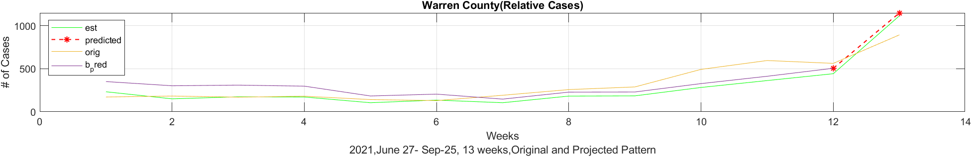
We implement a tensor completion algorithm to our tensor data. We replace the last (most current) week’s data of the Atlantic and Warren counties with the mean of the remaining data. Then, the missing values on the tensor is completed via low rank approximation of the Covid-19 tensor. We have the following very nice prediction; see Figures 18-22.


6 Future Works and Conclusion
In this work, we apply various tensor models and tensor algorithms to analyze Covid-19 data. The standard tensor models, CP and HOOI, with their off-the-shelves algorithms, ALS and HOOI, are tested against a new sampling method for ALS (SMALS). The numerical results are very promising as it cuts the down time while keeping the Frobenious norm errors relatively consistent with ALS. Here tensor sparse model [31, 8] is used as the model for prediction of future Covid-19 infection cases as a tensor completion problem. The numerical results are impressive as the tensor completion algorithm can predict infection a week ahead as well as a quarter ahead. Moreover, the tensor sparse model can locate which counties exhibit hotspots. The sparse tensor model is based on proximal algorithms and flexible hybrid method by Golub-Kahan methods for efficient practical implementation.
In our future work, we would like to have a more mathematical and methodical technique in locating and detecting hotspots. We have used minimization in the tensor completion; we will work on the efficacy of minimization of low-rank approximation of CP decomposition and tensor completion algorithm in the proximal framework.
Acknowledgments
This material is based upon work supported by the National Science Foundation under Grant No. DMS-1439786 while the author, C. Navasca, was in residence at the Institute for Computational and Experimental Research in Mathematics in Providence, RI, during the Model and Dimension Reduction in Uncertain and Dynamic Systems Program. C. Navasca is also in part supported by National Science Foundation No. MCB-2126374.
References
- [1] United states census bureau: New jersey population, GitHub repository, (2020).
- [2] P. Bejon, T. N. Williams, A. Liljander, A. M. Noor, J. Wambua, E. Ogada, A. Olotu, F. H. Osier, S. I. Hay, A. Färnert, and K. Marsh, Stable and unstable malaria hotspots in longitudinal cohort studies in Kenya, PLoS Med, 7 (2010), p. e1000304.
- [3] R. Bro, Parafac. tutorial and applications, Chemometrics and Intelligent Laboratory Systems, 38 (1997), pp. 149–171, https://doi.org/https://doi.org/10.1016/S0169-7439(97)00032-4, https://www.sciencedirect.com/science/article/pii/S0169743997000324.
- [4] L. De Lathauwer, B. De Moor, and J. Vandewalle, A multilinear singular value decomposition, SIAM Journal on Matrix Analysis and Applications, 21 (2000), pp. 1253–1278, https://doi.org/10.1137/S0895479896305696, https://doi.org/10.1137/S0895479896305696, https://arxiv.org/abs/https://doi.org/10.1137/S0895479896305696.
- [5] D. M. Dunlavy, T. G. Kolda, and E. Acar, Temporal link prediction using matrix and tensor factorizations, 5 (2011).
- [6] H. Ge, J. Caverlee, and H. Lu, Taper: A contextual tensor-based approach for personalized expert recommendation, in Proceedings of the 10th ACM Conference on Recommender Systems, RecSys ’16, New York, NY, USA, 2016, Association for Computing Machinery, p. 261–268.
- [7] C. J. Hillar and L.-H. Lim, Most tensor problems are np-hard, J. ACM, 60 (2013), https://doi.org/10.1145/2512329, https://doi.org/10.1145/2512329.
- [8] J. Jiang, F. Sanogo, and C. Navasca, Low-CP-rank tensor completion via practical regularization, J. Sci. Comput., 91 (2022), pp. Paper No. 18, 20, https://doi.org/10.1007/s10915-022-01789-9, https://doi.org/10.1007/s10915-022-01789-9.
- [9] A. Karatzoglou, X. Amatriain, L. Baltrunas, and N. Oliver, Multiverse recommendation: N-dimensional tensor factorization for context-aware collaborative filtering, in Proceedings of the Fourth ACM Conference on Recommender Systems, RecSys ’10, New York, NY, USA, 2010, Association for Computing Machinery, p. 79–86.
- [10] R. G. Karim, D. Dulal, and C. Navasca, Tensor decomposition via sampling methods, (2023).
- [11] R. G. Karim, G. Guo, D. Yan, and C. Navasca, Accurate tensor decomposition with simultaneous rank approximation for surveillance videos, in 2020 54th Asilomar Conference on Signals, Systems, and Computers, IEEE, 2020, pp. 842–846.
- [12] T. G. Kolda and B. W. Bader, Tensor decompositions and applications, SIAM Review, 51 (2009), pp. 455–500, https://doi.org/10.1137/07070111X.
- [13] J. Kruskal, Three-way arrays: rank and uniqueness of trilinear decompositions, with applications to arithmetic complexity and statistics, Linear Algebra Appl., 18 (1977), pp. 95–138.
- [14] J. Lessler, A. S. Azman, H. S. McKay, and S. M. Moore, What is a Hotspot Anyway?, Am J Trop Med Hyg, 96 (2017), pp. 1270–1273.
- [15] N. Li, S. Kindermann, and C. Navasca, Some convergence results on the regularized alternating least-squares method for tensor decomposition, 2011, https://doi.org/10.48550/ARXIV.1109.3831, https://arxiv.org/abs/1109.3831.
- [16] J. Liu, P. Musialski, P. Wonka, and J. Ye, Tensor completion for estimating missing values in visual data, in 2009 IEEE 12th International Conference on Computer Vision, 2009, pp. 2114–2121, https://doi.org/10.1109/ICCV.2009.5459463.
- [17] Y. Liu, F. Shang, H. Cheng, J. Cheng, and H. Tong, Factor matrix trace norm minimization for low-rank tensor completion, in SDM, 2014.
- [18] F. Liu , J. Chen , W. Tan , and C. Cai , A multi-modal fusion method based on higher-order orthogonal iteration decomposition, Entropy, 23 (2021), https://doi.org/10.3390/e23101349, https://www.mdpi.com/1099-4300/23/10/1349.
- [19] H. Lyu, C. Strohmeier, G. Menz, and D. Needell, COVID-19 time-series prediction by joint dictionary learning and online NMF, CoRR, abs/2004.09112 (2020), https://arxiv.org/abs/2004.09112, https://arxiv.org/abs/2004.09112.
- [20] J. Mathew, R. K. Behera, Z. E. Panthakkalakath, et al., A deep learning framework for covid outbreak prediction, arXiv preprint arXiv:2010.00382, (2020).
- [21] E. E. Papalexakis, C. Faloutsos, and N. D. Sidiropoulos, Tensors for data mining and data fusion: Models, applications, and scalable algorithms, ACM Trans. Intell. Syst. Technol., 8 (2016), https://doi.org/10.1145/2915921, https://doi.org/10.1145/2915921.
- [22] E. E. Papalexakis, C. Faloutsos, and N. D. Sidiropoulos, Tensors for data mining and data fusion: Models, applications, and scalable algorithms, ACM Trans. Intell. Syst. Technol., 8 (2017), pp. 16:1–16:44, https://doi.org/10.1145/2915921, https://doi.org/10.1145/2915921.
- [23] A. Preprint, Local convergence of the alternating least squares algorithm for canonical tensor approximation, SIAM Journal on Matrix Analysis and Applications, 33 (2012), https://doi.org/10.1137/110843587.
- [24] F. Sanogo and C. Navasca, Tensor completion via the cp decomposition, in 2018 52nd Asilomar Conference on Signals, Systems, and Computers, 2018, pp. 845–849, https://doi.org/10.1109/ACSSC.2018.8645405.
- [25] B. N. Sheehan and Y. Saad, Higher order orthogonal iteration of tensors (hooi) and its relation to pca and glram, in SDM, 2007.
- [26] N. D. Sidiropoulos, L. De Lathauwer, X. Fu, K. Huang, E. E. Papalexakis, and C. Faloutsos, Tensor decomposition for signal processing and machine learning, IEEE Transactions on Signal Processing, 65 (2017), pp. 3551–3582, https://doi.org/10.1109/TSP.2017.2690524.
- [27] Q. Song, H. Ge, J. Caverlee, and X. Hu, Tensor completion algorithms in big data analytics, 13 (2019), https://doi.org/10.1145/3278607, https://doi.org/10.1145/3278607.
- [28] N. Times, New jersey counties covid cases. https://github.com/nytimes/covid-19-data/blob/master/us-counties.csv.
- [29] H. Wang and N. Yamamoto, Using a partial differential equation with google mobility data to predict covid-19 in arizona, Mathematical Biosciences and Engineering, 17 (2020), pp. 4891–4904, https://doi.org/10.3934/mbe.2020266, https://www.aimspress.com/article/doi/10.3934/mbe.2020266.
- [30] X. Wang and C. Navasca, Adaptive low rank approximation of tensors, in Proceedings of the IEEE International Conference on Computer Vision Workshop (ICCVW, Santiago, Chile, 2015.
- [31] X. Wang and C. Navasca, Low-rank approximation of tensors via sparse optimization, Numer. Linear Algebra Appl., 25 (2018), pp. e2136, 17, https://doi.org/10.1002/nla.2136, https://doi.org/10.1002/nla.2136.
- [32] X. Wang and C. Navasca, Low-rank approximation of tensors via sparse optimization, Numerical Linear Algebra Appl., 25 (2018), pp. 2183–2202, https://doi.org/http://dx.doi.org/10.1002/andp.19053221004.
- [33] Z. Yang, Z. Zeng, K. Wang, S.-S. Wong, W. Liang, M. Zanin, P. Liu, X. Cao, Z. Gao, Z. Mai, J. Liang, X. Liu, S. Li, Y. Li, F. Ye, W. Guan, Y. Yang, F. Li, S. Luo, Y. Xie, B. Liu, Z. Wang, S. Zhang, Y. Wang, N. Zhong, and J. He, Modified seir and ai prediction of the epidemics trend of covid-19 in china under public health interventions, Journal of Thoracic Disease, 12 (2020), https://jtd.amegroups.com/article/view/36385.
- [34] Y. Zhao, H. Yan, S. E. Holte, R. P. Kerani, and Y. Mei, Rapid detection of hot-spot by tensor decomposition with application to weekly gonorrhea data, in International Workshop on Intelligent Statistical Quality Control, Springer, 2019, pp. 265–286.