Covariance Analysis of Impulsive Streaking

We first derive the impulsive model for $K[X,Y]$ in the absence of machine fluctuations, i.e. when the only variation in the measurement is $\bm{k}$, in which case $K[X,Y]=C[X,Y]$. As illustrated in Eqn. (3), in the impulsive regime $X(\bm{r})\simeq X^{0}(\bm{r}-\bm{k}_{X})$, and $Y(\bm{r})\simeq Y^{0}(\bm{r}-\bm{k}_{Y})$. Substituting the Taylor expansions of $X$ and $Y$ into the definition of covariance Eqn. (5), we find the leading order is

where $\nabla$ is the 2D momentum gradient operator, $R(-\phi)$ is the 2-by-2 matrix representing the counterclockwise rotation of $-\phi$ in the $xy$-plane. This leading order is the inner-product between $\nabla{X^{0}}$ and $R(-\phi)\nabla{Y^{0}}$, also referred to as the gradient inner-product (GIP), and the delay is encoded in the rotation.

In the impulsive regime, the streaking covariance defined in Eqn. (6) is given by a bilinear operation on the unstreaked distributions, $C[{\mathcal{D}}_{\bm{k}_{X}},{\mathcal{D}}_{\bm{k}_{Y}}]{X^{0}}{Y^{0}}$. As shown in Eqn. (7), the leading order in this bilinear operator $C[{\mathcal{D}}_{\bm{k}_{X}},{\mathcal{D}}_{\bm{k}_{Y}}]$ can be written as

where $\hat{G}(\phi)\equiv\lambda\sum_{i,j}R_{ij}(-\phi)\partial_{i}\otimes\partial_{j}$, with the direct product defined as $\partial_{i}\otimes\partial_{j}\equiv\frac{\partial}{\partial r_{q,i}}\frac{\partial}{\partial r_{p,j}}$ to perform partial differentiation with respect to momentum coordinates $\bm{r}_{q}$ and $\bm{r}_{p}$, respectively. The full expansion of $C[{\mathcal{D}}_{\bm{k}_{X}},{\mathcal{D}}_{\bm{k}_{Y}}]$ is

where $\hat{H}\equiv\left(\nabla^{2}\otimes\hat{I}+\hat{I}\otimes\lambda^{2}\nabla^{2}\right)/2$, $\hat{I}$ is the identity operator, and $\gamma_{n}\equiv\langle k^{2n}\rangle/(2^{2n}(n!)^{2})$. According to Eqn. (9), the streaking covariance expands into multiple direct products between the $n_{X}$-th order partial derivative of $X$ and the $n_{Y}$-th order partial derivative of $Y$. We number them by the differentiation orders $(n_{X}+n_{Y})$, e.g. the GIP term is the (1+1) order. The next orders are (1+3), (3+1), and (2+2), since all terms’ $(n_{X}+n_{Y})$ are even numbers, as shown by Eqn. (9).

In a measurement, we record electron yield with finite momentum resolution. We consider the covariance between the electron yield measured in two arbitrary regions $Q$ and $P$. Due to the bilinearity of covariance, this is identical to the regional integral of the covariance between the densities $X$ and $Y$:

As illustrated in Fig. 2, we define two sets of 2D momentum regions of interest (ROIs): $\{Q_{q}\}_{q=1}^{N_{Q}}$ for $X$ and $\{P_{p}\}_{p=1}^{N_{P}}$ for $Y$. We use subscripts $q,p$ on $X,Y$ as a shorthand for the regional integrals, e.g. $X_{q}\equiv\int_{Q_{q}}X(\bm{r})d^{2}\bm{r}$, as illustrated in Fig. 2. Fig. 3(a) shows an exemplary visualization of $K[X,Y]$, where the covariance has been calculated between $N_{Q}{=}N_{P}{=}180$ ROIs on the $p_{z}{=}0$ plane, each $2^{\circ}$-wide. The 180 angular bins are on a ring $p_{\mathrm{min}}<|\bm{r}|<p_{\mathrm{max}}$ and labelled by their central angular positions $\theta_{q}$ or $\theta_{p}$, thus they are also referred to as angular bins. In Fig. 3, both photoelectron features $X$ and $Y$ are simulated in the same ionization process as Fig. 1 but detected separately, and we set $\lambda=1$ to simulate the scenarios where the difference in photoemission delays is much shorter than the dressing field period $\omega|\tau_{X}-\tau_{Y}|\ll 1$. As shown in the $\phi=\pi/3$ example in Fig. 3(a), one feature of $K[X,Y]$ is that the most positive part is around $\theta_{p}-\theta_{q}\sim\phi$. At small streaking amplitudes, $K[X,Y]$ is well approximated by the GIP, as shown in Fig. 3(b-c). The the relative error $\|M_{\mathrm{GIP}}-K[X,Y]\|_{2}/\|K[X,Y]\|_{2}$ between panel (b) and (a) is evaluated as $0.03$, which we use to quantify the accuracy of the GIP. The accuracy of the GIP model is insensitive to $\phi$, but it degrades as streaking amplitude $k$ increases, due to the increased contribution from the higher order terms. As shown by the solid curve in Fig. 3(c), the root-mean-squared (rms) relative error over $\phi\in[-\pi,+\pi]$ becomes comparable to unity once $k$ exceeds the width of the photoelectron feature in momentum $\Delta p$ (quantified as the full-width at half-maximum, FWHM). For panels (a-b), the lower boundary $p_{\mathrm{min}}$ of the ROIs is set to the maximum point of the unstreaked MD gradient $p_{\mathrm{MG}}\equiv\arg\max_{r}\int d\theta|\nabla I^{0}|$  (red solid line in Fig. 3(d)), and the upper boundary is set to where the streaked MD has fallen to zero. This choice of limit for $p_{\min}$ optimizes the accuracy of the GIP model, because $p_{\mathrm{MG}}$ is close to the zero point of $\nabla^{2}I^{0}$. As shown in Fig. 3(c-d), when we alternate $p_{\min}$ by a fraction of $\Delta p$, the relative error is increased when $k/\Delta p<1$.

For the photoelectron features produced in direct ionization, the discrepancy between the GIP model and the streaking covariance $K[X,Y]$ generally depends on three characteristic dimensionless quantities: (1) the size of the momentum shift normalized to the momentum spread of the photoelectron feature $k/\Delta p$, (2) the normalized radius $p_{c}/\Delta p$, with $p_{c}$ denoting the central momentum of the photoelectron feature, and (3) the ratio of the ionizing pulse duration to the streaking laser period $\Delta t_{X}/T_{L}$. In the impulsive regime $\Delta t_{X}\ll T_{L}$, we find that the relative error is predominantly a function of $k/\Delta p$, with a much weaker dependence on $p_{c}/\Delta p$, as shown in Fig. 3(f). In the case shown in panels (a-e), both $X$ and $Y$ have a normalized radius of $p_{c}/\Delta p=6.6$, and when we vary $p_{c}/\Delta p$ by changing $\Delta t_{X}$ and/or the photon energy of the ionizing pulse, the relative error curve does not significantly change as long as we remain in the impulsive regime ($\Delta t_{X}\ll T_{L}$). The two features $X$ and $Y$ can have different $\Delta p_{X},\Delta p_{Y}$, but we note that by defining $\Delta p$ as the geometric mean $\Delta p=\sqrt{\Delta p_{X}\Delta p_{Y}}$, the accuracy of the GIP can be well described by $k/\Delta p$.

We differentiate the shot-to-shot fluctuations in angular streaking experiments into two categories, the fluctuation of the streaking vector $\bm{k}$, and everything else. The fluctuations of these other parameters (or “machine fluctuations”), such as pulse energy and central photon energy of the ionizing pulse, also affect the single-shot MD, but the relative timing between the ionizing and dressing pulses typically does not depend on these parameters. Thus in this work, machine fluctuations are assumed to be statistically independent from the random streaking vector. The streaking covariance $K[X,Y]$ defined in Eqn. (6) is therefore simplified by the impulsive condition as $K[X,Y]\simeq C[\mathcal{D}_{\bm{k}_{X}}\langle X^{0}\rangle,\mathcal{D}_{\bm{k}_{Y}}\langle Y^{0}\rangle]$. We note that the expected dressing-free MDs $\langle X^{0}\rangle,\langle Y^{0}\rangle$ are fixed, free from shot-to-shot variations, so the treatment of $K[X,Y]$ introduced in Sec. II.1 are also applicable when machine fluctuations are present, by simply replacing the stable $X^{0},Y^{0}$ with $\langle X^{0}\rangle,\langle Y^{0}\rangle$ respectively.

Both machine fluctuations and fluctuations in $\bm{k}$ contribute to the covariance $C[X,Y]$ defined in Eqn. (5). According to the law of total covariance [24], $C[X,Y]=K[X,Y]+L[X,Y]$ consists of the streaking covariance $K[X,Y]$ defined in Eqn. (6) and the contribution from machine fluctuations:

where in the approximation, we used the impulsive streaking condition and the statistical independence between machine fluctuations and streaking vector.

To retrieve the delay, the GIP model of $K[X,Y]$ relies on the gradients $\nabla X_{q},\nabla Y_{p}$:

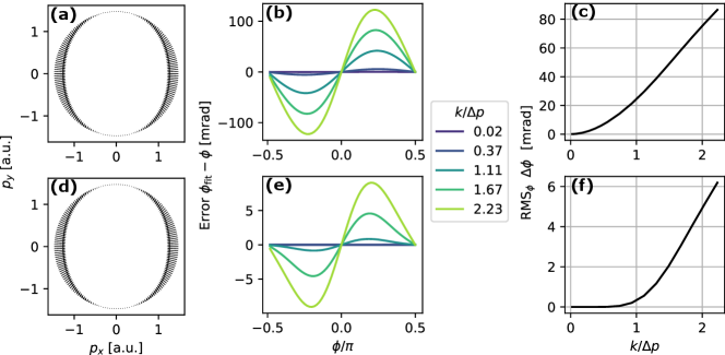
One way to reconstruct the gradients $\nabla X_{q},\nabla Y_{p}$ is through numerical differentiation (ND). Dressing-free shots provide the sample mean of the measured distributions $\overline{X^{0}}$ and $\overline{Y^{0}}$ to estimate the expectations $\langle X^{0}\rangle$ and $\langle Y^{0}\rangle$, respectively. With adequate momentum resolution, we can use a finite difference scheme to numerically differentiate $\overline{X^{0}}$, and then integrate over $Q_{q}$ to measure the gradient $\nabla X_{q}$. An example is shown in Fig. 5(a) for the case in Fig. 1 &3. Obtaining the gradients $\nabla X_{q},\nabla Y_{p}$ from numerical differentiation, we fit the GIP model to the sample streaking covariance $\mathrm{K}_{XY}$, with the factor $\langle k^{2}\rangle\lambda$ treated as a free parameter in Eqn. (12). Because the amplitude ratio $\lambda$ has been absorbed into the free scaling parameter, not knowing $\lambda$ does not affect this method. We benchmark the accuracy of the ND method in the noiseless limit: i.e. with sufficient number of shots $N_{s}\to\infty$ to suppress statistical noise, complete removal of machine fluctuations, and ignoring readout noise in the electron yield. Thus we equate $\mathrm{K}_{XY}$ to the underlying $K[X,Y]$ and obtain the delay retrieval error $\Delta\phi=\phi_{\mathrm{fit}}-\phi$ at various “ground-truth” $\phi$, Fig. 5(b). This systematic error is zero when $\phi$ is a multiple of $\pi/2$ and reaches a maximum at $\phi\,{\sim}\pm\pi/4$. The rms error over $\phi$ increases with $k$ due to the increase in higher-order terms, as shown in panel (c), but within $k<\Delta p$ this rms error is $<0.03\,\mathrm{rad}{=}1.7^{\circ}$, which converts to a time delay error $<30\,\mathrm{as}$ for a $2\,\mathrm{\mu m}$-wavelength dressing field.

Another way to reconstruct the gradient is “rank-reduction” (RR), described in Algorithm 1, which employs a low-rank approximation of $K[X,X]$ and $K[Y,Y]$ to estimate the gradient. This method can be used when each set of ROIs complete a loop on the high-momentum side of the corresponding photoelectron feature, e.g. the rings delineated in Fig. 4. Within the GIP model, $K[X_{q},X_{q^{\prime}}]=\langle k^{2}/2\rangle(\nabla X_{q})^{T}\nabla X_{q^{\prime}}$, whose rank is at most 2 since $\nabla X_{q}$ is 2D. Thus it appears we can solve the following optimization problem given $\mathrm{K}_{XX}$:

where $\xi=(\xi_{1},\cdots,\xi_{N_{Q}})\in\mathbb{R}_{2{\times}N_{Q}}$ represents the gradient field, $a_{q}$ is the arc length of the angular bin at $\theta_{q}$ and $W$ is a $N_{Q}\times N_{Q}$ matrix weights, which can be configured to combat the effect of readout noise as described below. The reconstructed gradient field is given by the optimal point $\xi^{*}$ of Eqn. (13) up to a global factor, $\xi_{q}^{*}=\sqrt{\langle k^{2}/2\rangle}\nabla X_{q}$. Applying the same procedure to $\mathrm{K}_{YY}$, we obtain the optimal point $\eta^{*}_{p}=\sqrt{\langle k^{2}/2\rangle}\lambda\nabla Y_{p}$. Thus the GIP model described in Eqn. (7) can be rewritten as $M_{\mathrm{GIP}}=(\xi^{*})^{T}R(-\phi)\eta^{*}$, which we then substitute into Eqn. (12) to retrieve $\phi_{\mathrm{fit}}$.

The minimization of the objective function $f_{\mathrm{RR}}$ is closely related to principal component analysis (PCA). The weight matrix can be configured as uniform $W_{qq^{\prime}}=1$ when the signal-to-noise ratio is high in the electron yield readout process. When the readout signal-to-noise ratio is low, we recommend ignoring the diagonal band of $\mathrm{K}_{XX}$ by setting the diagonal band in $W$ to zero (e.g. $W_{qq^{\prime}}=1-\delta_{qq^{\prime}}$). Guidance for defining is detailed in Sec. IV.2. With a uniform $W$, a minimal point of $f_{\mathrm{RR}}$ is given by the PCA result $\xi^{\mathrm{P}}=\left(\sqrt{s^{(1)}}v^{(1)},\sqrt{s^{(2)}}v^{(2)}\right)^{T}$ [25], where $s^{(\alpha)}$ is the $\alpha$-th largest eigenvalue of $\mathrm{K}_{XX}$ and $v^{(\alpha)}$ is the corresponding eigenvector (in column vector form). When $W$ is non-uniform, e.g. $W_{qq^{\prime}}=1-\delta_{qq^{\prime}}$, we can minimize $f_{\mathrm{RR}}$ by optimizing $\xi^{\mathrm{P}}$ using gradient descent.

The objective function $f_{\mathrm{RR}}$ is invariant under any global orthogonal transformation $O{:}~{}\xi_{q}\mapsto O\xi_{q}$, but only certain minimal points can satisfy the zero-loop constraint Eqn. (13b), which is a general property of a gradient field $\oint\nabla X^{0}\cdot d\bm{l}=0$. Thus obtaining one minimal point $\xi^{\mathrm{P}}$, we solve for an orthogonal matrix $O$ such that $l_{\mathrm{RR}}(O\xi^{\mathrm{P}})=0$ This is straightforwardly achieved by parameterizing $O$ with the rotation angle and parity. An alternative to the zero-loop constraint is maximizing the gradient-flux $j_{\mathrm{RR}}(O\xi^{\mathrm{P}})\equiv-\sum_{q}(\cos\theta_{q},~{}\sin\theta_{q})O\xi^{\mathrm{P}}_{q}a_{q}$ with $O$, which necessarily satisfies the zero-loop constraint and additionally breaks the remaining discrete degeneracy, as proven in Supplemental Sec. 2.

Similar to the results in Fig. 5(b-c), we benchmark the RR method under various $\phi$ and $k$ in the noiseless limit as mentioned above, as shown in panels (d-f). The gradient fields $\nabla X_{q}$ and $\nabla Y_{p}$ are reconstructed from $\mathrm{K}_{XX}$ and $\mathrm{K}_{YY}$, respectively, and we show the resultant $\nabla X_{q}$ in panel (d). Similar to the ND method, the delay retrieval error of the RR method is minimized when $\phi$ is a multiple of $\pi/2$. The rms error increases with $k$, but the magnitude of the error is notably smaller than with the ND method. As shown in Fig. 5(f), the rms error is ${<}1$ mrad within $k{<}\Delta p$, corresponding to ${<}1$ as for a $2\,\mathrm{\mu m}$ dressing field.

The main reason for the higher accuracy of the RR method lies in the reconstructed “gradient”. The ND gradients give the first-order derivatives of the dressing-free MD $\nabla X_{q}$ and $\nabla Y_{p}$, independent from the streaking amplitude $k$. The gradient reconstructed by the RR procedure, in contrast, deviates from the first-order derivative as $k$ increases. To the next lowest order, the RR gradients are

which include the third-order derivatives in addition to the first-order (see Supplementary Sec. 1.2). As a result, when using the RR gradients, the inner product $\xi_{q}^{T}R(\phi)\eta_{p}$ not only captures the (1+1) order of $K[X_{q},Y_{p}]$, but also the (1+3) and (3+1) orders. In contrast when using the ND gradient, only the (1+1) order is modelled. Since the errors in the noiseless limit arise from the finite accuracy of the GIP model and are insensitive to the normalized radius $p_{c}/\Delta p$, the result in Fig. 5 is general across $p_{c}/\Delta p$.

In some experiments, gradient reconstruction may be challenging. For example, the numerical differentiation becomes infeasible when the detector lacks angular resolution, and RR becomes infeasible when the available ROIs cannot complete a loop. In this case, it is often possible to identify a part of the streaking correlation matrix $R[X_{q},Y_{p}]\equiv{K[X_{q},Y_{p}]}/{\sqrt{K[X_{q},X_{q}]K[Y_{p},Y_{p}]}}$ that can be used to extract the photoemission delay without requiring knowledge of the gradient.

In the angular regions where the gradient is predominantly along the radial direction $|r^{-1}\partial_{\theta}X_{q}|\ll|\partial_{r}X_{q}|$, $|r^{-1}\partial_{\theta}Y_{p}|\ll|\partial_{r}Y_{p}|$ (also referred to as the “radial regions”), the streaking covariance is approximated as

The $\cos(\phi-\theta_{p}+\theta_{q})$ factor explains the positive ridge around $\theta_{p}-\theta_{q}{\sim}\phi$ in the covariance matrix. The radial gradients in Eqn. (15), including the factor $\lambda$, cancel out, i.e. $R\left[X_{q},Y_{p}\right]\approx\cos(\phi-\theta_{p}+\theta_{q})$. Therefore we define the gradient-free model as $M_{\mathrm{GF}}\equiv a\cos(\phi-\theta_{p}+\theta_{q})$, with free parameters $a$ and $\phi$. From the measured K-estimators, we calculate the sample correlation matrix $\mathrm{Corr}_{XY}=\mathrm{K}_{XY}/\sqrt{\mathrm{K}_{XX}\mathrm{K}_{YY}}$, and minimize the mean-squared error in the radial region between $\mathrm{Corr}_{XY}$ and the model $M_{\mathrm{GF}}$.

The radial region is determined from the dressing-free MD. For the case shown in Figs. 3 and 5, the anisotropy parameter is $\beta_{2}=2$, the radial region defined by $|r^{-1}\partial_{\theta}X_{q}|<0.2|\partial_{r}X_{q}|$ is $138^{\circ}$-wide around each antinode of the dipole feature. For lower anisotropy parameters, the radial region is larger, since an isotropic feature has no angular gradient component. As shown in Fig. 6(a), within the radial region, the correlation matrix is well described by the gradient-free model $M_{\mathrm{GF}}$. By fitting $M_{\mathrm{GF}}$ to the measured $\mathrm{Corr}_{XY}$ in the radial region, we obtain $\phi_{\mathrm{fit}}$, and the error $\phi_{\mathrm{fit}}-\phi$ is shown in Fig. 6(b & c). Similar to the gradient-based methods, the error is zero at $\phi=0,\pm\pi/2$, but the rms error across $\phi\in[0,2\pi]$ does not vanish when $k\to 0$. This residual error at small streaking amplitude arises from ignoring the non-radial regions, and in the case shown in Fig. 6, it amounts to $20$ mrad rms. The systematic error of the gradient-free method also increases with $k$, but the increase is slower than for the ND method. In this case, comparing Fig. 6(c) to Fig. 5(c), we find the gradient-free method is more accurate than the ND method when $k\gtrsim\Delta p$, but remains less accurate than the RR method. Another difference between the gradient-free and gradient-based methods is the dependence on $p_{c}/\Delta p$: the gradient-free method is generally more accurate with higher $p_{c}/\Delta p$, since the magnitude of the radial gradient relative to the angular gradient increases.

When implementing analysis procedures that make use of fluctuations in the measured data, it is important to understand how instabilities in the measurement affect the measured correlation, in this case $\mathrm{C}_{XY}$. When using an attosecond x-ray free electron laser there may be fluctuations in the x-ray parameters, for example the pulse energy and/or the central photon energy. In this section we describe how to manage the effect of these additional fluctuations in the delay extraction procedure.

References

- The Nobel Committee for Physics [2023] The Nobel Committee for Physics, Scientific background to the nobel prize in physics 2023 (2023).
- Itatani et al. [2002] J. Itatani, F. Quéré, G. L. Yudin, M. Y. Ivanov, F. Krausz, and P. B. Corkum, Attosecond Streak Camera, Physical Review Letters 88, 173903 (2002).
- Bradley et al. [1971] D. Bradley, B. Liddy, and W. Sleat, Direct linear measurement of ultrashort light pulses with a picosecond streak camera, Optics Communications 2, 391 (1971).
- Thumm et al. [2015] U. Thumm, Q. Liao, E. M. Bothschafter, F. Süßmann, M. F. Kling, and R. Kienberger, Attosecond physics: Attosecond streaking spectroscopy of atoms and solids, in Photonics (John Wiley & Sons, Ltd, 2015) Chap. 13, pp. 387–441, https://onlinelibrary.wiley.com/doi/pdf/10.1002/9781119009719.ch13 .
- Schultze et al. [2010] M. Schultze, M. Fieß, N. Karpowicz, J. Gagnon, M. Korbman, M. Hofstetter, S. Neppl, A. L. Cavalieri, Y. Komninos, T. Mercouris, C. A. Nicolaides, R. Pazourek, S. Nagele, J. Feist, J. Burgdörfer, A. M. Azzeer, R. Ernstorfer, R. Kienberger, U. Kleineberg, E. Goulielmakis, F. Krausz, and V. S. Yakovlev, Delay in Photoemission, Science 328, 1658 (2010).
- Drescher et al. [2002] M. Drescher, M. Hentschel, R. Kienberger, M. Uiberacker, V. Yakovlev, A. Scrinzi, T. Westerwalbesloh, U. Kleineberg, U. Heinzmann, and F. Krausz, Time-resolved atomic inner-shell spectroscopy, Nature 419, 803 (2002).
- Eckle et al. [2008] P. Eckle, A. N. Pfeiffer, C. Cirelli, A. Staudte, R. Dörner, H. G. Muller, M. Büttiker, and U. Keller, Attosecond Ionization and Tunneling Delay Time Measurements in Helium, Science 322, 1525 (2008).
- Hartmann et al. [2018] N. Hartmann, G. Hartmann, R. Heider, M. S. Wagner, M. Ilchen, J. Buck, A. O. Lindahl, C. Benko, J. Grünert, J. Krzywinski, J. Liu, A. A. Lutman, A. Marinelli, T. Maxwell, A. A. Miahnahri, S. P. Moeller, M. Planas, J. Robinson, A. K. Kazansky, N. M. Kabachnik, J. Viefhaus, T. Feurer, R. Kienberger, R. N. Coffee, and W. Helml, Attosecond time–energy structure of X-ray free-electron laser pulses, Nature Photonics 12, 215 (2018).
- Duris et al. [2020] J. Duris, S. Li, T. Driver, E. G. Champenois, J. P. MacArthur, A. A. Lutman, Z. Zhang, P. Rosenberger, J. W. Aldrich, R. Coffee, G. Coslovich, F.-J. Decker, J. M. Glownia, G. Hartmann, W. Helml, A. Kamalov, J. Knurr, J. Krzywinski, M.-F. Lin, J. P. Marangos, M. Nantel, A. Natan, J. T. O’Neal, N. Shivaram, P. Walter, A. L. Wang, J. J. Welch, T. J. A. Wolf, J. Z. Xu, M. F. Kling, P. H. Bucksbaum, A. Zholents, Z. Huang, J. P. Cryan, and A. Marinelli, Tunable isolated attosecond X-ray pulses with gigawatt peak power from a free-electron laser, Nature Photonics 14, 30 (2020), number: 1 Publisher: Nature Publishing Group.
- Franz et al. [2024] P. Franz, S. Li, T. Driver, R. R. Robles, D. Cesar, E. Isele, Z. Guo, J. Wang, J. P. Duris, K. Larsen, J. M. Glownia, X. Cheng, M. C. Hoffmann, X. Li, M.-F. Lin, A. Kamalov, R. Obaid, A. Summers, N. Sudar, E. Thierstein, Z. Zhang, M. F. Kling, Z. Huang, J. P. Cryan, and A. Marinelli, Terawatt-scale attosecond X-ray pulses from a cascaded superradiant free-electron laser, Nature Photonics 18, 698 (2024), publisher: Nature Publishing Group.
- Haynes et al. [2021] D. C. Haynes, M. Wurzer, A. Schletter, A. Al-Haddad, C. Blaga, C. Bostedt, J. Bozek, H. Bromberger, M. Bucher, A. Camper, S. Carron, R. Coffee, J. T. Costello, L. F. DiMauro, Y. Ding, K. Ferguson, I. Grguraš, W. Helml, M. C. Hoffmann, M. Ilchen, S. Jalas, N. M. Kabachnik, A. K. Kazansky, R. Kienberger, A. R. Maier, T. Maxwell, T. Mazza, M. Meyer, H. Park, J. Robinson, C. Roedig, H. Schlarb, R. Singla, F. Tellkamp, P. A. Walker, K. Zhang, G. Doumy, C. Behrens, and A. L. Cavalieri, Clocking Auger electrons, Nature Physics , 1 (2021), publisher: Nature Publishing Group.
- Li et al. [2022] S. Li, T. Driver, P. Rosenberger, E. G. Champenois, J. Duris, A. Al-Haddad, V. Averbukh, J. C. T. Barnard, N. Berrah, C. Bostedt, P. H. Bucksbaum, R. N. Coffee, L. F. DiMauro, L. Fang, D. Garratt, A. Gatton, Z. Guo, G. Hartmann, D. Haxton, W. Helml, Z. Huang, A. C. LaForge, A. Kamalov, J. Knurr, M.-F. Lin, A. A. Lutman, J. P. MacArthur, J. P. Marangos, M. Nantel, A. Natan, R. Obaid, J. T. O’Neal, N. H. Shivaram, A. Schori, P. Walter, A. L. Wang, T. J. A. Wolf, Z. Zhang, M. F. Kling, A. Marinelli, and J. P. Cryan, Attosecond coherent electron motion in Auger-Meitner decay, Science 375, 285 (2022), publisher: American Association for the Advancement of Science.
- Guo et al. [2024] Z. Guo, T. Driver, S. Beauvarlet, D. Cesar, J. Duris, P. L. Franz, O. Alexander, D. Bohler, C. Bostedt, V. Averbukh, X. Cheng, L. F. DiMauro, G. Doumy, R. Forbes, O. Gessner, J. M. Glownia, E. Isele, A. Kamalov, K. A. Larsen, S. Li, X. Li, M.-F. Lin, G. A. McCracken, R. Obaid, J. T. O’Neal, R. R. Robles, D. Rolles, M. Ruberti, A. Rudenko, D. S. Slaughter, N. S. Sudar, E. Thierstein, D. Tuthill, K. Ueda, E. Wang, A. L. Wang, J. Wang, T. Weber, T. J. A. Wolf, L. Young, Z. Zhang, P. H. Bucksbaum, J. P. Marangos, M. F. Kling, Z. Huang, P. Walter, L. Inhester, N. Berrah, J. P. Cryan, and A. Marinelli, Experimental demonstration of attosecond pump–probe spectroscopy with an X-ray free-electron laser, Nature Photonics 18, 691 (2024), publisher: Nature Publishing Group.
- Maroju et al. [2020] P. K. Maroju, C. Grazioli, M. Di Fraia, M. Moioli, D. Ertel, H. Ahmadi, O. Plekan, P. Finetti, E. Allaria, L. Giannessi, G. De Ninno, C. Spezzani, G. Penco, S. Spampinati, A. Demidovich, M. B. Danailov, R. Borghes, G. Kourousias, C. E. Sanches Dos Reis, F. Billé, A. A. Lutman, R. J. Squibb, R. Feifel, P. Carpeggiani, M. Reduzzi, T. Mazza, M. Meyer, S. Bengtsson, N. Ibrakovic, E. R. Simpson, J. Mauritsson, T. Csizmadia, M. Dumergue, S. Kühn, H. Nandiga Gopalakrishna, D. You, K. Ueda, M. Labeye, J. E. Bækhøj, K. J. Schafer, E. V. Gryzlova, A. N. Grum-Grzhimailo, K. C. Prince, C. Callegari, and G. Sansone, Attosecond pulse shaping using a seeded free-electron laser, Nature 578, 386 (2020).
- Maroju et al. [2023] P. K. Maroju, M. Di Fraia, O. Plekan, M. Bonanomi, B. Merzuk, D. Busto, I. Makos, M. Schmoll, R. Shah, P. R. Ribič, L. Giannessi, G. De Ninno, C. Spezzani, G. Penco, A. Demidovich, M. Danailov, M. Coreno, M. Zangrando, A. Simoncig, M. Manfredda, R. J. Squibb, R. Feifel, S. Bengtsson, E. R. Simpson, T. Csizmadia, M. Dumergue, S. Kühn, K. Ueda, J. Li, K. J. Schafer, F. Frassetto, L. Poletto, K. C. Prince, J. Mauritsson, C. Callegari, and G. Sansone, Attosecond coherent control of electronic wave packets in two-colour photoionization using a novel timing tool for seeded free-electron laser, Nature Photonics 17, 200 (2023), number: 2 Publisher: Nature Publishing Group.
- Driver et al. [2024] T. Driver, M. Mountney, J. Wang, L. Ortmann, A. Al-Haddad, N. Berrah, C. Bostedt, E. G. Champenois, L. F. DiMauro, J. Duris, D. Garratt, J. M. Glownia, Z. Guo, D. Haxton, E. Isele, I. Ivanov, J. Ji, A. Kamalov, S. Li, M.-F. Lin, J. P. Marangos, R. Obaid, J. T. O’Neal, P. Rosenberger, N. H. Shivaram, A. L. Wang, P. Walter, T. J. A. Wolf, H. J. Wörner, Z. Zhang, P. H. Bucksbaum, M. F. Kling, A. S. Landsman, R. R. Lucchese, A. Emmanouilidou, A. Marinelli, and J. P. Cryan, Attosecond delays in X-ray molecular ionization, Nature 632, 762 (2024), publisher: Nature Publishing Group.
- Wang et al. [2024] J. Wang, T. Driver, P. L. Franz, P. Kolorenč, E. Thierstein, R. R. Robles, E. Isele, Z. Guo, D. Cesar, O. Alexander, S. Beauvarlet, K. Borne, X. Cheng, L. F. DiMauro, J. Duris, J. M. Glownia, M. Graßl, P. Hockett, M. Hoffman, A. Kamalov, K. A. Larsen, S. Li, X. Li, M.-F. Lin, R. Obaid, P. Rosenberger, P. Walter, T. J. Wolf, J. P. Marangos, M. F. Kling, P. H. Bucksbaum, A. Marinelli, and J. P. Cryan, Probing electronic coherence between core-level vacancies at different atomic sites, Physical Review X (accepted) (2024).
- Haynes et al. [2020] D. C. Haynes, M. Wurzer, A. Schletter, A. Al-Haddad, C. Blaga, C. Bostedt, J. Bozek, M. Bucher, A. Camper, S. Carron, R. Coffee, J. T. Costello, L. F. DiMauro, Y. Ding, K. Ferguson, I. Grguraš, W. Helml, M. C. Hoffmann, M. Ilchen, S. Jalas, N. M. Kabachnik, A. K. Kazansky, R. Kienberger, A. R. Maier, T. Maxwell, T. Mazza, M. Meyer, H. Park, J. S. Robinson, C. Roedig, H. Schlarb, R. Singla, F. Tellkamp, K. Zhang, G. Doumy, C. Behrens, and A. L. Cavalieri, Clocking Auger Electrons, arXiv:2003.10398 [physics] (2020), arXiv: 2003.10398.
- Kitzler et al. [2002] M. Kitzler, N. Milosevic, A. Scrinzi, F. Krausz, and T. Brabec, Quantum Theory of Attosecond XUV Pulse Measurement by Laser Dressed Photoionization, Physical Review Letters 88, 173904 (2002).
- Wolkow [1935] D. M. Wolkow, Über eine Klasse von Lösungen der Diracschen Gleichung, Zeitschrift für Physik 94, 250 (1935).
- Li et al. [2018] S. Li, E. G. Champenois, R. Coffee, Z. Guo, K. Hegazy, A. Kamalov, A. Natan, J. O’Neal, T. Osipov, M. Owens, D. Ray, D. Rich, P. Walter, A. Marinelli, and J. P. Cryan, A co-axial velocity map imaging spectrometer for electrons, AIP Advances 8, 115308 (2018), publisher: American Institute of Physics.
- Glownia et al. [2010] J. M. Glownia, J. Cryan, J. Andreasson, A. Belkacem, N. Berrah, C. I. Blaga, C. Bostedt, J. Bozek, L. F. DiMauro, L. Fang, J. Frisch, O. Gessner, M. Gühr, J. Hajdu, M. P. Hertlein, M. Hoener, G. Huang, O. Kornilov, J. P. Marangos, A. M. March, B. K. McFarland, H. Merdji, V. S. Petrovic, C. Raman, D. Ray, D. A. Reis, M. Trigo, J. L. White, W. White, R. Wilcox, L. Young, R. N. Coffee, and P. H. Bucksbaum, Time-resolved pump-probe experiments at the LCLS, Optics Express 18, 17620 (2010).
- Kheifets et al. [2022] A. S. Kheifets, R. Wielian, V. V. Serov, I. A. Ivanov, A. L. Wang, A. Marinelli, and J. P. Cryan, Ionization phase retrieval by angular streaking from random shots of XUV radiation, Physical Review A 106, 033106 (2022), publisher: American Physical Society.
- DeGroot and Schervish [2010] M. H. DeGroot and M. J. Schervish, Probability and Statistics, 4th ed. (Pearson, Upper Saddle River, NJ, 2010) p. 261.
- Eckart and Young [1936] C. Eckart and G. Young, The approximation of one matrix by another of lower rank, Psychometrika 1, 211 (1936).
- Johnson and Wichern [2007] R. A. Johnson and D. W. Wichern, in Applied Multivariate Statistical Analysis (Pearson, Upper Saddle River, NJ, 2007) 6th ed., pp. 407–410.
- Walter et al. [2021] P. Walter, A. Kamalov, A. Gatton, T. Driver, D. Bhogadi, J.-C. Castagna, X. Cheng, H. Shi, R. Obaid, J. Cryan, W. Helml, M. Ilchen, and R. N. Coffee, Multi-resolution electron spectrometer array for future free-electron laser experiments, Journal of Synchrotron Radiation 28, 1364 (2021).
- Petkovšek et al. [1996] M. Petkovšek, H. S. Wilf, and D. Zeilberger, A=B (A K Peters, Wellesley, MA, 1996) p. 38.