Coupling Diffusion and Finite Deformation in Phase Transformation Materials
Abstract
We present a multiscale theoretical framework to investigate the interplay between diffusion and finite lattice deformation in phase transformation materials. In this framework, we use the Cauchy-Born Rule and the Principle of Virtual Power to derive a thermodynamically consistent theory coupling the diffusion of a guest species (Cahn-Hilliard type) with the finite deformation of host lattices (nonlinear gradient elasticity). We adapt this theory to intercalation materials—specifically Li1-2Mn2O4—to investigate the delicate interplay between Li-diffusion and the cubic-to-tetragonal deformation of lattices. Our computations reveal fundamental insights into the microstructural evolution pathways under dynamic discharge conditions, and provide quantitative insights into the nucleation and growth of twinned microstructures during intercalation. Additionally, our results identify regions of stress concentrations (e.g., at phase boundaries, particle surfaces) that arise from lattice misfit and accumulate in the electrode with repeated cycling. These findings suggest a potential mechanism for structural decay in Li2Mn2O4. More generally, we establish a theoretical framework that can be used to investigate microstructural evolution pathways, across multiple length scales, in first-order phase transformation materials.
keywords:
First-order phase transformation , Lattice deformation , Intercalation material , Phase-field methods , Energy storage1 Introduction
First-order phase transformation materials undergo an abrupt change in lattice geometries at critical temperature, stress, or composition values. In intercalation compounds, a type of first-order phase transformation material, lattices deform abruptly and often anisotropically when guest species (e.g., ions, atoms, or molecules) are inserted into the material (Padhi et al., 1997; Whittingham, 1978). The reversible insertion of guest species makes intercalation materials suitable for applications in energy storage, optoelectronics, and catalysis (Wan et al., 2016), and are widely used as electrodes in rechargeable batteries. The reversible lattice deformation is commonly of two types: First, the deformation is dilatational (e.g., in LiFePO4 or LiCoO2 compounds) in which the unit cells expand/contract without a change in symmetry (Padhi et al., 1997). Second, the deformation is symmetry-lowering in which unit cells undergo a change in symmetry type (e.g., cubic-to-tetragonal in Li2Mn2O4) during transformation (Thackeray et al., 1983). These lattice deformations are viewed as the root cause leading to the structural decay of intercalation materials and are often suppressed during reversible cycling (Bai et al., 2011; Zhang et al., 2021).
By contrast, we show that symmetry-lowering lattice deformations can be systematically designed to mitigate structural degradation in intercalation materials Zhang and Balakrishna (2023); Balakrishna (2022); Schofield et al. (2022). We developed algorithms to screen lattice deformations in pairs of intercalation compounds and, found that several intercalation materials, such as the Spinels and NASICONs, undergo a symmetry-lowering transformation and can form shape-memory-like microstructures Zhang and Balakrishna (2023). These lattice deformations can be designed (e.g., through substitutional doping Schofield et al. (2022); Santos et al. (2023)), to minimize volume changes and interfacial stresses. However, to guide this design methodology, we need a robust and quantitative theoretical model that predicts how individual lattices deform and interact with the Li-diffusion front at the atomic scale, and how this interplay in turn governs the macroscopic material response. In this work, we develop a theoretical framework to investigate the interplay between diffusion and finite lattice deformation in symmetry-lowering phase transformation materials.

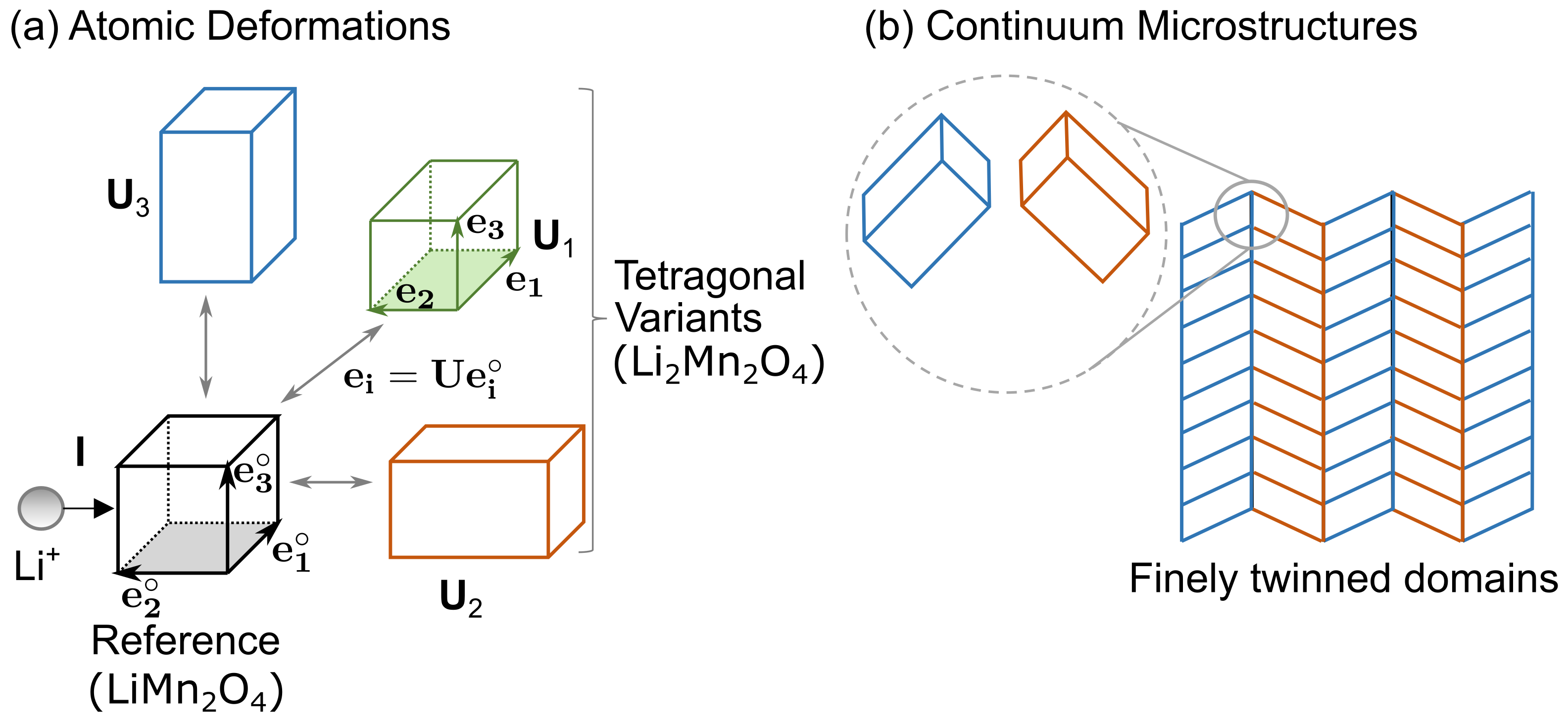
Symmetry-lowering phase transformations generate complex microstructural patterns, see Fig. 1(a-b) (Erichsen et al., 2020). The origins of these finely twinned domains can be explained as a consequence of energy minimization (Ball and James, 1987). For example, the cubic to tetragonal transformation in Li1-2Mn2O4 generates significant misfit strains between the cubic-LiMn2O4 and the tetragonal-Li2Mn2O4 lattices. To minimize this elastic energy tetragonal lattices rotate and shear to form twinned domains at the continuum scale. This finely twinned mixture reduces the average misfit strains with the cubic phase, and thereby, minimizes the total elastic energy stored in the system. These microstructures can be analyzed using elastic energy arguments, however, it is important to understand how these microstructures interact with the diffusion of guest-species (e.g., Li-ions) and how this interplay, in turn, governs macroscopic material response such as internal stresses and micro-cracking, see Fig. 1(c) (Luo et al., 2020; Balakrishna, 2022).
At present, mesoscale models predict phase transformations in intercalation materials using guest-species composition (e.g., Li-ion) as the order parameter (Zhang and Kamlah, 2019; Tang et al., 2010; Nadkarni et al., 2019; Ombrini et al., 2023; Han et al., 2004; Zhang and Kamlah, 2020). In these methods lattice deformations are typically homogenized and the free energy potential does not distinguish between the different lattice variants generated during symmetry-lowering phase transformations. Consequently, these models predict phase separation morphologies as a function of a scalar composition variable and are not suitable for investigating the rich heterogeneity in lattice deformations. These phase-field methods effectively predict reaction heterogeneities (Han et al., 2004), redox potentials (Ombrini et al., 2023), and particle size effects (Tang et al., 2010; Zhang and Kamlah, 2019) under electrochemical operating conditions, however, they do not account for higher-order energy terms necessary to predict how twinned microstructures nucleate and grow during phase transformations.
Researchers have developed phenomenological methods that couple strain and composition fields within a single framework (Rudraraju et al., 2014, 2016; Balakrishna and Carter, 2018; Balakrishna et al., 2019). For example, a chemo-mechanical model based on strain gradient elasticity theory describes the diffusion-driven martensitic phase transformations in multi-component crystalline solids (Rudraraju et al., 2016). In another example, we combined a Cahn-Hilliard model with a phase-field crystal model to investigate diffusion-induced stresses in binary alloys (Balakrishna and Carter, 2018). These methods provide important insights into the coupling between higher-order diffusion and nonlinear strain gradient terms. These models, however, are based on variational derivations of the free energy functions that require a-priori specification and do not rigorously account for rate terms in deriving the governing equations (Gurtin, 1996, 2002; Di Leo et al., 2014; Anand, 2012). Moreover, the dynamic electrochemical operating conditions driving phase transformations in intercalation compounds are not formulated in these frameworks. We will build on these efforts, to derive a thermodynamically consistent multiscale theory to investigate the diffusion-deformation interplay in phase transformation materials.
Our central aim is to establish a thermodynamically consistent framework that couples the diffusion of guest-species with the finite deformation of host lattices in phase transformation materials. To this end, we use the Cauchy-Born Rule and the Principle of Virtual Power to systematically derive the form of the free energy function and the governing equations for the diffusion-deformation model. We adapt this theoretical framework to intercalation materials by introducing specialized constitutive equations to capture the electrochemical operating conditions. We next solve this theoretical framework using a mixed-type finite element formulation based on Lagrange multipliers and calibrate the model to a spinel-type Li2xMn2O4 electrode as a representative example. Our results yield fundamental insights into the interplay between Li-diffusion and heterogeneous lattice deformations in Li2xMn2O4 during phase transformations. In line with experimental observations, our simulations successfully predict the geometric features of the finely twinned domains, and microstructural evolution pathways, and quantitatively estimate the macroscopic material response (e.g., voltage curves, stress distributions) during a galvanostatic discharge half cycle in Li2Mn2O4. Additionally, our simulations reveal significant interfacial stresses at phase boundaries and particle surfaces, which suggest a potential mechanism for failure in Li2xMn2O4. Broadly, our results highlight the use of our modeling framework to investigate and design crystallographic microstructures in first-order phase transformation materials.
2 Theory
In this section we use the Cauchy-Born Rule (Ericksen, 2008) and the Principle of Virtual Power (Gurtin, 2002; Anand, 2012) and the Thermodynamic principles to derive the constitutive form of the diffusion-deformation theory. We start by analyzing the lattice deformations in Li2Mn2O4, as a representative compound, and formulate a thermodynamically consistent framework to predict symmetry-lowering phase transformations in chemo-mechanical materials.
2.1 Kinematics
Consider a body occupying a region in three-dimensional Euclidean space in the reference configuration. Let be the position of a point on in this reference configuration. We describe the deformation of this body as a function , in which denotes the position of point in the deformed configuration. Given any deformation , we describe the deformation gradient as a matrix of partial derivatives with components,
| (1) |
We use to denote this deformation gradient, i.e., a rank-2 tensor and the gradient operator is calculated with respect to the reference configuration. Please note, in this work, we denote vectors and tensors using bold lower-case and upper-case Roman letters, respectively. We denote the components of these vectors and tensors, with respect to a Cartesian basis, using upper-case (lower-case) indices in the reference (deformed) configuration. A vector with a hat is a unit normal vector (e.g., ) in the reference configuration.
2.2 Bravais Lattices
In the continuum theory of crystalline solids, the Cauchy-Born rule, relates the movement of atoms in a crystal to the overall deformation of the body. That is, consider the body as described above, and at each point , there is a Bravais lattice that defines the crystalline arrangement of atoms. This Bravais lattice is an infinite set of points in three-dimensional space that can be generated by the translation of a single point through three linearly independent lattice vectors . In the reference configuration, the unit cell is defined by lattice vectors and deforms according to the deformation gradient:
| (2) |
We define the Green-Lagrange strain tensor as
| (3) |
in which is the identity matrix. The strain tensor in coordinate notation is given by .
The Cauchy-Born rule gives an exact correspondence between these structural transformations of individual lattices and continuum microstructures at a material point. For example, in first-order phase transformation materials (i.e., materials undergoing displacive-type of transformation), we describe the structural transformation of lattices using a positive-definite symmetric matrix
| (4) |
Fig. 2(a) shows a cubic-to-tetragonal deformation of lattices with the three tetragonal variants described by , and , respectively. In intercalation materials, such as Li2Mn2O4, a similar displacive-type of lattice transformation is observed using in-situ TEM.
2.3 Compatibility Conditions
During phase transformation, the tetragonal variants rotate and fit compatibly with each other forming energy-minimizing deformations called twin interfaces. That is, two lattice variants described by transformation matrices and satisfy the Hadamard jump condition (or the Kinematic compatibility condition):
| (5) |
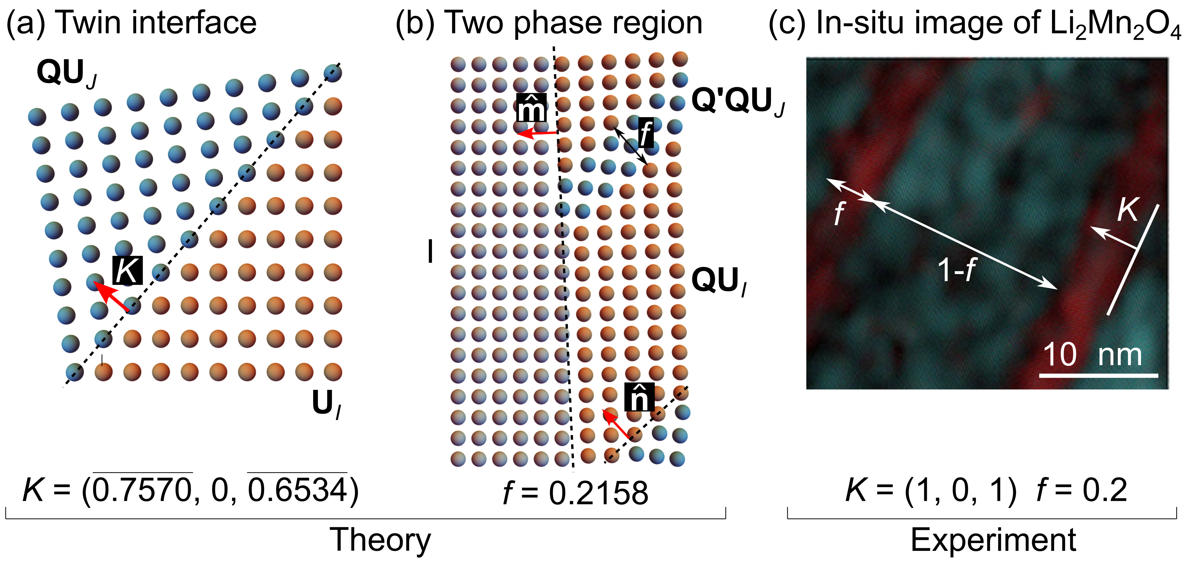
for a given rotation matrix and vectors and , see Fig. 3. The solution to Eq. (5) then describes a twin plane that connects the two lattice variants and coherently. These twin interfaces have been observed in intercalation materials, such as Li2Mn2O4, in-situ, during battery operation. These twin interfaces are rarely found in isolation. As illustrated in Fig. 3, finely twinned microstructures form when any two lattice variants, with deformation tensors and , satisfy the kinematic compatibility condition for some scalar (Ball and James, 1987; Bhattacharya, 2003):
| (6) |
Here the reference cubic lattice is represented by , rotation matrices by and , and vectors and . These martensite-like microstructures describe energy-minimizing deformations that reduce coherency stresses at the phase boundary and, arise from the multi-well structure of the energy landscape. We discuss this in detail in section 6.1.
In our recent work (Zhang and Balakrishna, 2023), we used compatibility conditions in Eqs. (5) and (6) to analytically construct the twin interfaces in Li2xMn2O4. As shown in Fig. 3, our analytical solutions of both the twin plane and the volume fraction for the austenite-martensite microstructure are consistent with experimental measurements (Erichsen et al., 2020). These observations further support our efforts to derive a diffusion-deformation model to predict crystallographic microstructures in Li2Mn2O4.
2.4 Mass Balance
Consider any spatial region inside the reference body , with an outward normal and a boundary . The diffusion of species (e.g., Li-ions in batteries) across this boundary is accompanied by a change in the species concentration and characterized by a flux . That is, the rate of change of the chemical species across is given by
| (7) |
Using the Divergence theorem over the integral we have,
| (8) |
Note that the choice of was arbitrary, and therefore the local mass balance law is as follows
| (9) |
2.5 Force Balance
The principle of virtual power states that there exists a fundamental power balance between the external power expended on , and the internal power expended within . To obtain the expressions for external and internal powers, we follow Gurtin (2002) and Anand (2012) and use “rate-like” kinematic descriptors — , , , , and — to derive the associated balance of forces by the principle of virtual power. These rates are not independent but are constrained by:
| (10) |
| External Power Internal Power | |||
| Force | Power | Force | Power |
| Conjugate | Conjugate | ||
| Traction | Stress | ||
| Moment | Higher-order stress | ||
| Line force | Scalar microscopic force | ||
| Body force | Vector microscopic force | ||
| Scalar microscopic traction | |||
In Table LABEL:Tab:1 we identify individual force systems expending power externally on and expending power internally within . We use these individual force systems to construct the total external and internal power as follows:
| (11) |
Please note that in Eq. (2.5) the stresses , , and microscopic forces and are defined over the body at all times. We define a line force across the boundary edge of the region . We assume that at any given time, the fields , , and are known, and we consider the fields , , and as virtual velocities. We specify each of these virtual velocities independently and keep them consistent with Eq. (10). Next, we introduce virtual fields of the form , , and , to distinguish these fields from the previously described virtual velocities (as associated with the real-time evolution of the body) and we ensure that virtual fields satisfy:
| (12) |
We define a generalized virtual velocity list that is consistent with Eq. (12). Following Anand (2012) and Gurtin (2002), we assume that under a change in the frame, the fields comprising the generalized virtual velocity convert as their nonvirtual counterparts. That is,
| (13) |
The external and internal power expenditures, respectively, are:
| (14) |
| (15) |
Power Balance: Given any spatial region ,
| (16) |
Frame-Indifference: Given any spatial region and any generalized virtual velocity ,
| (17) |
To deduce the outcomes of the principle of virtual power, we assume that Eqs. (16) and (17) are satisfied. We note that in applying the virtual balance described by Eq. (16), we are free to choose any that is consistent with the constraint Eq. (12).
2.5.1 Macroscopic Force and Moment Balances
Let us assume . For this choice of the generalized virtual velocity , the constraint in Eq. (12) and the Power Balance requirement in Eq. (16) yield:
| (18) |
We systematically simplify Eq. (18) (see the detailed steps in Appendix A) and derive the macroscopic force balance. For our purposes, we list the form of this force balance
| (19) | |||||
Here is a surface gradient operator and . Eq. (19) holds for all choices of and and, the standard variational arguments, respectively, lead to the following traction conditions:
| (20) |
and the local macroscopic force balance:
| (21) |
The principle of frame-indifference Eq. (17) (underlying most physical laws including the principle of virtual power) requires that the internal power is invariant to all changes of frame :
| (22) |
in which is the generalized virtual velocity in the new frame. In this new frame, is transformed to , and are transformed according to Eq. (13). Scalar fields, such as and , are frame invariant and, gradient fields, such as is equal to . With these transformations, a change in frame converts internal power to
| (23) | |||||
Since is an arbitrary part of the reference body , we have
| (25) |
Note that this change in frame can be arbitrary and we can proceed in two ways. First, we assume a time-independent rotation, , and we have:
| (26) |
As Eq. (26) must hold for all , , and , the stresses and need to satisfy
| (27) |
and the microstress is invariant
| (28) |
Second, we assume a change of frame satisfying , such that is an arbitrary skew tensor. With this assumption, we obtain
| (29) |
and the stress is symmetric,
| (30) |
2.5.2 Microscopic Force Balance
We next analyze the microscopic counterparts of the macroscopic force balance. We consider a generalized virtual velocity with and an arbitrary virtual field . By substituting these fields into the external and internal power expenditures, Eqs. (14) and (15), and together with the power balance requirement of the principle of virtual power Eq. (16) and the constraint Eq. (12), we have the following microscopic virtual-power relation:
| (31) |
Eq. (31) holds for all values of and for all choices of . By applying the divergence theorem, we have
| (32) |
Eq. (32) must hold for all choices of and all , standard variational arguments yield the microscopic traction condition:
| (33) |
and the microscopic force balance:
| (34) |
2.6 Imbalance of Energy
We next derive the free energy imbalance under isothermal conditions. Let represent the Helmholtz free energy density of the system per unit volume and represent the chemical potential of the diffusing species in the reference configuration. By neglecting the kinetic energy of the system, we have:
| (35) |
Using the power balance property , Eq. (2.5) and the divergence theorem, we have:
| (36) |
Using the mass balance from Eq. (9) and noting that Eq. (36) holds for all spatial regions , we write the local form of the free energy imbalance as:
| (37) |
In Eq. (37), we introduce a net chemical potential,
| (38) |
At this point, we define a dissipation density per unit volume per unit time:
| (39) |
2.7 Constitutive Theory
We next consider the constitutive forms for the free energy density , the first Piola-Kirchhoff stress tensor , the third-order stress tensor , the net chemical potential , and the vector microscopic force , and the species flux . Following the free energy imbalance derived in Eq. (37), we note that each term can be expressed as a functional of the deformation gradient , species concentration , and the chemical potential :
| (40) |
Substituting the constitutive forms in Eq. (2.7) into the free-energy imbalance in Eq. (37), and using the chain rule, we have
| (41) |
This above inequality holds for all values of , , , and , which, in Eq. (41) appear in a linear form. The corresponding coefficients of these fields must vanish, so that , , , and can not be chosen to violate the free energy imbalance in Eq. (41). This argument, consequently, leads to the following thermodynamic restriction in which the first Piola-Kirchhoff stress , the third-order stress , the chemical potential , and the vector microscopic force are defined as derivatives of the free energy function :
| (42) |
In Eq. (2.7), please note that the symmetry condition for third-order stress is . The dissipation inequality introduced in Eq. (39) reduces to
| (43) |
Recalling the definition of in Eq. (38) and by using the constitutive form for in Eq. (2.7) and the microforce balance for in Eq. (34), we derive the constitutive equation for the chemical potential:
| (44) |
We note that the form of the chemical potential in Eq. (44), derived from a microforce balance and thermodynamically consistent constitutive relations, is the same as the chemical potential obtained from a variational derivative of the energy functional (Rudraraju et al., 2016; Zhang and Kamlah, 2018).
Finally, we write the constitutive form of the flux of the diffusing species in Eq. (2.7) as:
| (45) |
in which is a mobility tensor. Substituting Eq. (45) in Eq. (43), we express the dissipation inequality as:
| (46) |
The inequality in Eq. (46) requires the mobility tensor to be a positive-semidefinite quantity.
3 Constitutive Theory for Intercalation Materials
The theory presented in section 2 is general and applicable to all first-order phase transformation materials, undergoing a symmetry-lowering lattice transformation. We next adapt this theory for intercalation materials, by introducing special constitutive equations that are relevant for modeling the Cahn-Hilliard type of diffusion and couple it with the structural transformations of lattices.
3.1 Free Energy Density
We now propose a free energy density for intercalation materials undergoing a symmetry-lowering lattice transformation. This energy density is applicable to other chemo-mechanically coupled phase transformation materials undergoing a displace-type of transformation.
Let us begin with the free energy density that depends on the lattice deformation gradient , and the concentration of diffusing species , . We assume that this free energy density is defined and continuous for all and and for all values of the species concentration during composition evolution. Here denotes a set of real matrices. We assume that the free energy is Galilean invariant: for all , for all values of around the critical point, and each orthogonal rotations with , we have:
| (47) |
Or equivalently, we describe the free energy in terms of the symmetric Green-Lagrange strain tensor from Eq. (3) , such that:
| (48) |
Furthermore, we assume that the free energy density is an isotropic function of its arguments, and consequently depends only on the magnitude of the gradient terms and ,
| (49) |
We note that this free energy density satisfies frame-indifference and material symmetry, i,e., for all rotations and is a finite point group of the undistorted crystalline lattice. The free energy density therefore satisfies:
| (50) |
The free energy density in Eq. (50) is a higher-order polynomial of its arguments and has a multi-well landscape. This together with the the higher-rank tensors in Eq. (50) introduces nonlinearities making it a challenge to numerically solve the free energy functional. We overcome some of these challenges, by writing the free energy density in terms of a symmetry-adapted strain measure vector :
| (51) |
Following (Barsch and Krumhansl, 1984; Thomas and Van der Ven, 2017), we use to describe the symmetry-breaking structural transformations of the lattices. The components of this strain measure are in turn a linear combination of the Green-Lagrange strain tensor components. That is, the strain measures are defined using the Green-Lagrange strain tensor components in three dimensions as follows:
| (52) |
We note that within the limits of a small deformation framework, represents a stretch-like deformation, and , and describe the shear-like deformation of lattices. The strain measures and in Eq. (3.1) not only assume different values in relation to a high-symmetry cubic lattice and a lower-symmetry tetragonal lattice, but also assume separate values to differentiate among the three tetragonal lattice variants. This construction of and , therefore, is most suitable as structural order parameters describing the cubic-to-tetragonal lattice transformations in intercalation materials.
It follows from Eqs. (50) and (51) that the free energy density satisfying both frame-indifference and material-symmetry is
| (53) |
and holds for all . In this work, we assume a zero vector minimizes the free energy density in the reference state and a non-zero tensor minimizes the free energy in the intercalated state. The invariant condition in Eq. (53) implies that if a pair minimizes , so is for each . These minimizers correspond to the different variants of the lower-symmetry phase and contribute to the multi-well energy landscape of the free energy function.
We next prescribe the specific form of the free energy function. We start by decomposing the free energy density into bulk and gradient energy terms. The bulk energy, in turn, includes contributions from the thermodynamic, elastic, and chemo-mechanically coupled terms:
| (54) | |||||
We construct the thermodynamic energy contribution as a sum of an ideal solution entropy and an excess free energy—representing a deviation from thermodynamic ideality—using a Redlich-Kirster polynomial series (Redlich and Kister, 1948):
| (55) |
Eq. (55) describes an energy landscape, which distinguishes between the reference and intercalated phases, as a function of the normalized concentration (scaled with the maximum species concentration as ). The constants, and correspond to the gas constant and the reference temperature, respectively. The Redlich-Kirster coefficients are obtained from the least square method and represent the excess energy contribution.
The elastic energy term penalizes the bulk and shear deformations:
| (56) |
The coefficients and correspond to the bulk and shear modulus, respectively, and represents the volume change associated with the cubic to tetragonal structural transformation of the host lattices.
Following Shchyglo et al. (2012); Barsch and Krumhansl (1984); Ahluwalia et al. (2006), we next construct the coupled chemo-mechanical energy term that describes a multi-well energy landscape in terms of order parameters . This energy landscape governs the cubic to tetragonal lattice transformation:
| (57) |
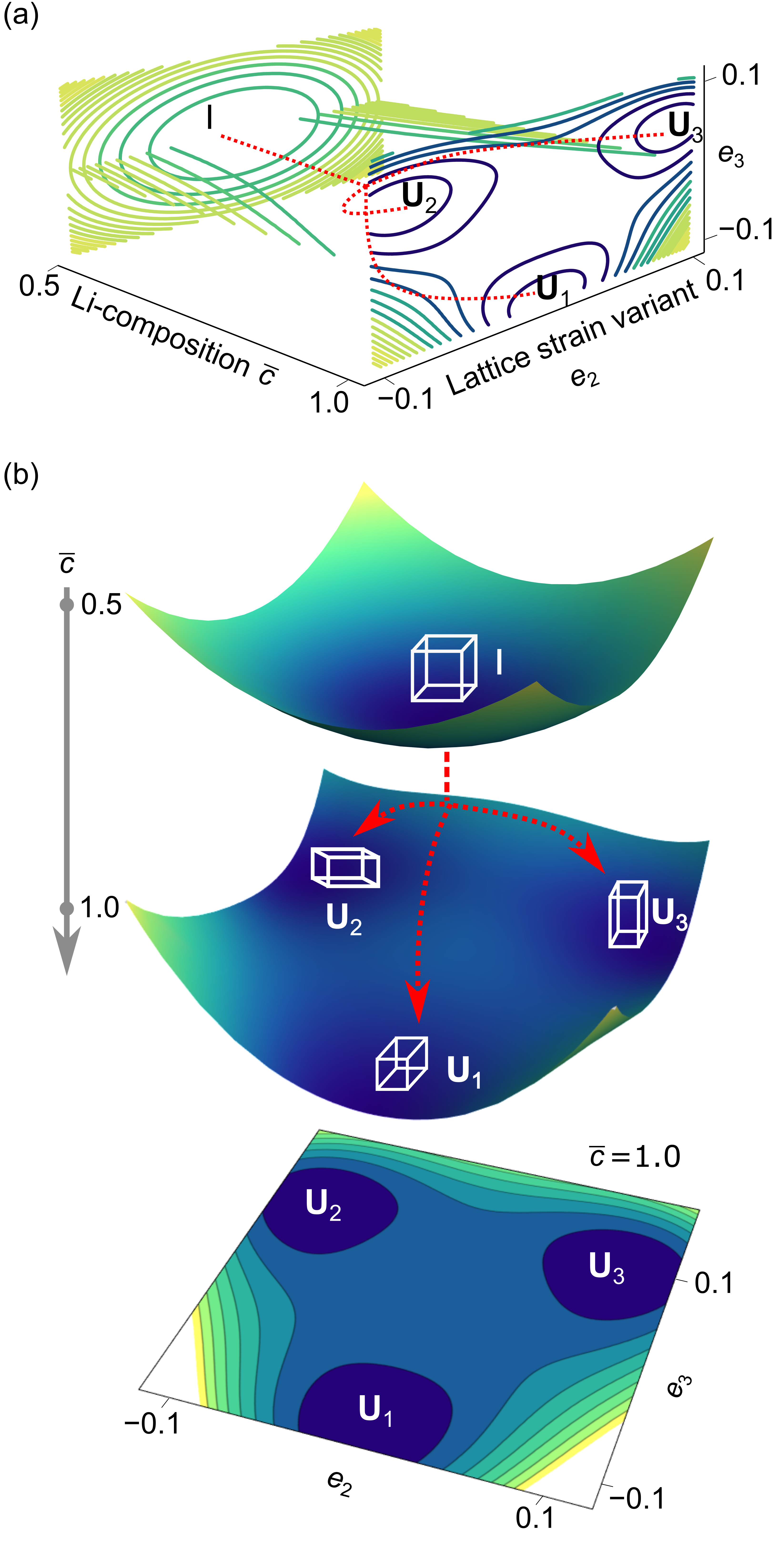
The coefficient represents the concentration-dependent deviatoric modulus governing the cubic to tetragonal transformations. The coefficients and are the nonlinear elastic constants. The third-order terms accompanying concentration-dependent coefficient are required to describe a first-order type of phase-transformation (Cowley, 1976). Fig. 4(a-b) shows three-dimensional plots of the free energy as a function of strain measure components , and normalized concentration . The energy well at corresponds to the higher-symmetry cubic phase (denoted by Identity tensor ) and the energy wells at corresponds to the tetragonal variants (denoted by stretch tensors ) at the lower-symmetry phase.
Finally, the gradient energy term penalizes changes in concentration and/or strain and is given by:
| (58) | |||||
In Eq. (58) we only include energy contributions from the quadratic gradient terms that also account for the mixed terms between and . These gradient terms describe nonlocal elastic and composition behavior, and their corresponding coefficients, in their general forms, are tensors that can be functions of both concentration and strain. Specifically, the concentration gradient energy coefficient is denoted by a symmetric tensor, the strain gradient energy coefficients are denoted by tensors for each combination of , and mixed gradient energy coefficient(s) is a tensor for . Eqs. (55)-(58) collectively construct the total free energy density.
3.2 Stress, Chemical Potential, and Microscopic Force
We next derive the constitutive equations for the stresses, chemical potential, and microscopic forces for the form of the free energy function in Eq. (54). Using Eqs. (54) and (2.7a) the first Piola-Kirchhoff stress tensor is given by:
| (59) |
We discretize these constitutive equations and implement them in a finite element framework in section 4.
3.3 Electrochemical reaction
During intercalation a guest-species, such as lithium, is inserted into the host-material lattices. This insertion is accompanied by an electrochemical reaction, at the electrode/electrolyte interface, which can be described for any guest species ‘A’ as follows:
| (63) |
We incorporate this electrochemical reaction in our constitutive model by using a phenomenological Butler-Volmer equation (Bai et al., 2011; Mykhaylov et al., 2019; Ganser et al., 2019) and describing the reaction rate. The Butler-Volmer reaction relates the current density to surface overpotential at the interface between electrode and electrolyte as:
| (64) |
In Eq. (64) is the electron-transfer symmetry factor, and is the Faraday constant. The exchange current density given by:
| (65) |
with denoting the reaction rate constant (units of ) and denoting the chemical potential in the electrolyte. We assume that the guest-species moves much faster in the electrolyte than in the active host material and therefore set (Bai et al., 2011). We define the surface overpotential as
| (66) |
where is the voltage drop across the interface between electrode and electrolyte. This voltage drop serves as a driving force for species insertion (or removal) into the electrode.
By combining Eqs. (64)-(66) we write the species flux at the electrode/electrolyte interface as:
| (67) |
Eq. (67) is important in modeling the galvanostatic boundary conditions for a battery electrode. For example, in this work we model the galvanostatic charge and discharge boundary conditions by employing the Butler-Volmer equation Eq. (67) on the electrode surface. On all reactive boundaries we model a global flux [mol/s] by summing over each boundary as follows:
| (68) |
In Eq. (68) the C-rate is defined as the rate of time (in hours) required to charge or discharge a battery and is divided by 3600 to keep all time-related units in seconds. We use Eqs. (66)-(68) to compute the voltage drop across the electrode/electrolyte surface as described in Appendix B.
Finally, we introduce Damköhler number to compare the reaction and diffusion time scales:
| (69) |
where is the characteristic length scale in the model, and is the diffusion coefficient. For a more detailed description of the galvanostatic (dis-)charging using the Butler-Volmer equation, we refer the reader to Appendix B.
3.4 Governing Equations and Boundary Conditions
In this section we summarize the governing equations and boundary conditions for an intercalation material undergoing a first-order symmetry-lowering phase transformation:
- •
-
•
Macroscopic Force Balance: We use the local force balance law in Eq. (21):
(71) In Eq. (71) represents the non-inertial body force, and the stresses and are given by Eq. (59) and Eq. (60), respectively. Please note that the higher-order stresses are often absent in traditional elasticity problems, however, we include these stresses in our work making the local force balance a fourth-order nonlinear PDE. This introduces additional challenges in solving the numerics that we discuss in the next section.
-
•
Mechanical Boundary Conditions: To define the mechanical boundary conditions on the intercalation material, we consider are complementary subsurfaces of the boundary, in which the motion is specified on and the surface traction on . denotes a smooth boundary edge on which a jump in higher-order stress traction may occur (Toupin, 1962). Considering the symmetry condition of , boundary conditions are finally given by:
(72) The Dirichlet boundary condition in Eq. (• ‣ 3.4a) is of the same form that appears in classical non-gradient elasticity problems. However, its complementary Neumann boundary condition described in Eq. (• ‣ 3.4b) contains higher-rank tensors that introduce complexity in gradient-type elasticity problems (e.g., in the present work). In addition to Eqs. (• ‣ 3.4a) and (• ‣ 3.4b), we follow Toupin’s theory (Toupin, 1962) and introduce a higher-order Neumann boundary condition for the higher-order stress traction in Eq. (• ‣ 3.4c). This form of stress traction does not have a boundary mechanism to impose a generalized moment across atomic bonds, and it is therefore defined on surface . Finally, Eq. (• ‣ 3.4d) ensures that there exists no discontinuity of higher-order stress traction across a smooth boundary edge in the absence of a balancing line traction (Toupin, 1962). We model these boundary conditions in the finite element framework as described in section 4.
-
•
Diffusion Boundary Conditions: Similar to the case of describing mechanical boundary conditions, we next consider are complementary subsurfaces of the boundary, in which the species concentration is specified on and the global flux on :
(73) Next, we note that the microscopic stresses contribute to a power expenditure by the material that is in contact with the body. This requires that we consider suitable boundary conditions on that involve the microscopic tractions and the rate of change of the species concentration . In this work, we restrict to boundary conditions resulting in a null power expenditure:
(74) A simple boundary condition which satisfies this null expenditure of microscopic power is given by:
(75) -
•
Initial Conditions: The initial conditions are
(76)
4 Numerical Implementation
We next outline the finite element implementation of diffusion and finite deformation theory for intercalation materials. We note that this is a coupled, nonlinear, initial boundary value problem, in which, both the Cahn-Hilliard type of diffusion and nonlinear gradient elasticity formulation are solved. These formulations include fourth-order spatial derivatives and higher-order boundary conditions, which make the computation cumbersome. For example, the numerical solutions to the fourth-order partial differential equations (Eqs. (70) and (71)) require -continuous finite elements and, the standard -continuous Lagrange basis functions are not sufficient. In order to reduce these continuity requirements, we follow Shu et al. (1999), and develop a mixed-type finite element formulation using Lagrange multipliers. In our framework, we introduce deformation gradient and chemical potential as additional degrees of freedom, and use mixed-methods to numerically solve the higher-order diffusion and nonlinear strain gradient elasticity problem.
4.1 Macroscopic Force Balance
Recall that the local force balance on Eq. (71) in the absence of non-inertial body force is
| (77) |
We introduce the deformation gradient as an additional degree of freedom and enforce kinematic constraints using a Lagrange multiplier :
| (78) |
The Galerkin weak form of the mixed formulation, with suitable test functions , are given by:
| (79) |
| (80) |
| (81) |
The corresponding forms using index notation are given by:
| (82) |
| (83) |
| (84) |
4.2 Mass Balance
The mass balance law in Eq. (70) involves fourth-order spatial derivatives in concentration and third-order spatial derivatives in displacement, and the standard finite element method with C0-continuous Lagrange basis functions are not sufficient for discretization. To overcome this numerical obstacle, we introduce the chemical potential as an additional degree of freedom and split the fourth-order PDE in Eq. (70) into two second-order equations. First, is the expression for chemical potential as given by Eq. (61) with the independent variable . Second, is the concentration evolution expression described in terms of the independent variable :
| (88) |
We next multiply Eq. (61) and Eq. (88) with variational test functions and , respectively, and integrate these equations over . For Eq. (61), we have:
| (89) | |||||
Similarly, for Eq. (88), we have:
| (90) |
4.3 Finite Element Implementation
We implement the above weak forms in the open source finite-element, multiphysics framework MOOSE (Gaston et al., 2009). We solve the system of nonlinear equations using the preconditioned Jacobian Free Newton Krylov (PJFNK) method. This approach does not require defining an explicit tangent matrix and therefore saves considerable computational time and storage. We use the implicit Backward-Euler method for time integration and an adaptive time-stepping approach for the relatively smooth diffusion process.
5 Application to Li2xMn2O4
We next calibrate the material coefficients for Li2xMn2O4 () that undergoes a cubic-to-tetragonal lattice deformation during intercalation. For simplicity, we assume a two-dimensional form of the model with . This assumption in turn reduces the strain measures in Eq. (3.1) to:
| (91) |
with and . We therefore construct the free energy in 2D as a function of the and, furthermore, in the absence of experimental measurements of gradient energies, we assume the most basic expression for the gradient energy contribution. Specifically, we assume an isotropic form for the gradient energy coefficients and , respectively. In the latter term, we only assume gradient energy contributions involving and set all other coefficients to zero. The coefficient accompanying the mixed composition-strain gradient term is also set to zero, . With these simplifications, the form of gradient energy density, with scalar constants and , for Li2xMn2O4 reduces to Eq. (5c) and the entire form of the 2D free energy density at is given as:
| (92) |
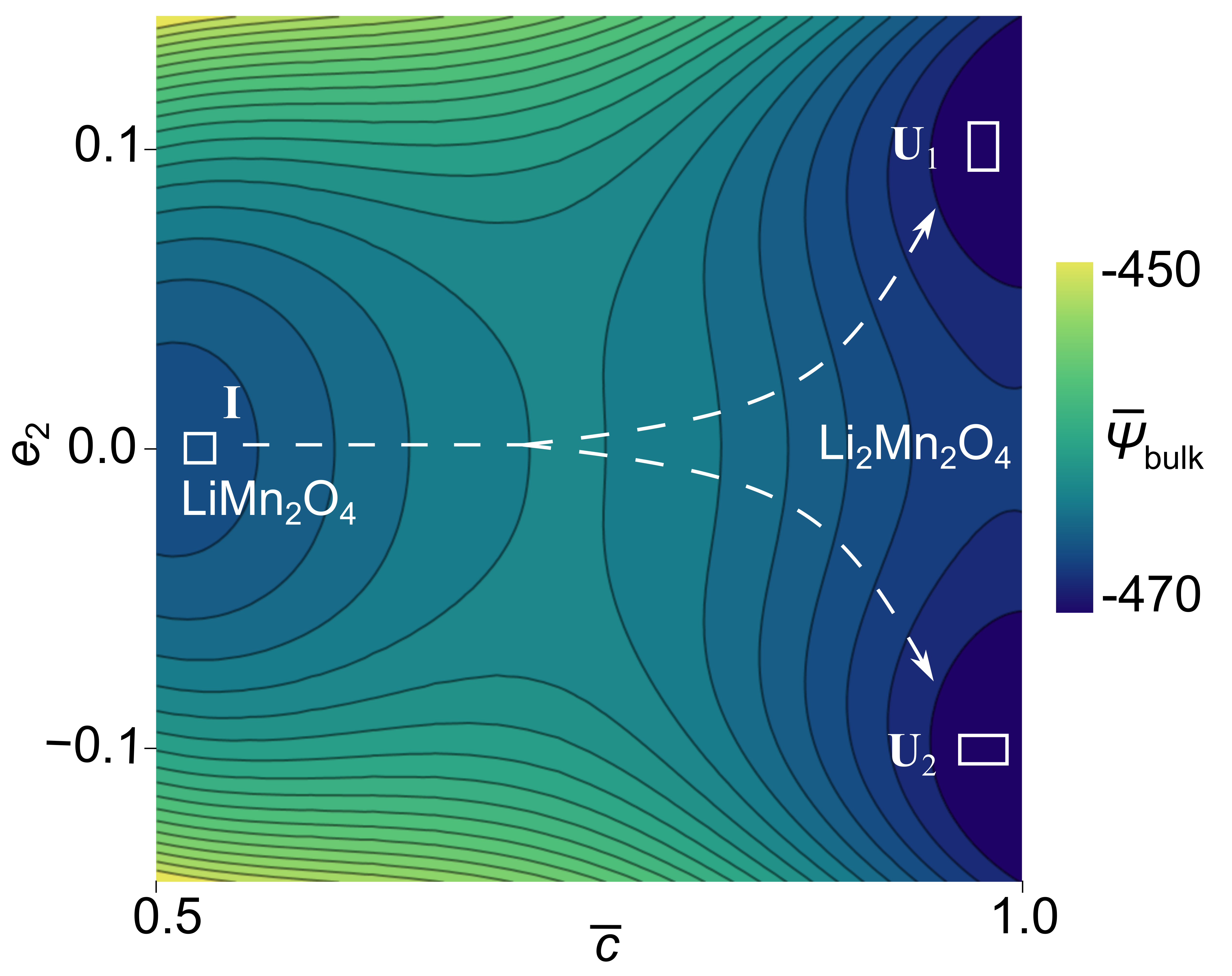
We note that in 2D, the free energy density is a functional of , , , , and and Fig. 5 shows the multi-well energy landscape as a function of and . In Fig. 5, the free energy density has minima at corresponding to the lithium-poor phase LiMn2O4 and at corresponding to the lithium-rich Li2Mn2O4 phase, respectively. The two energy wells of equal height at correspond to the two lattice variants in 2D.
Moving forward, we nondimensionalize the total of the system as . We fit the coefficients of the thermodynamic energy term in Eq. (5a) with the phase segregation thermodynamics of Li2xMn2O4. Specifically, we fit the Open Circuit Voltage (OCV) parameters with the experimental measurements from Thackeray et al. (1983), as shown in Fig. 6(a). The specific values of the Redlich-Kirster and the reference chemical potential coefficients are listed in Table 2. For these combinations of coefficients, the Legendre transformation of the Helmholtz free energy density reduces to (Hörmann and Groß, 2019; Nadkarni et al., 2019):
| (93) |
Eq. (93) describes a doublewell structure with minima at and , corresponding to the Li-poor (LiMn2O4) and Li-rich (Li2Mn2O4) phases, respectively, see Fig. 6(b).
We next calibrate the coefficients in the elastic and the coupled energy terms for Li2xMn2O4:
| (94) |
In Eq. (94) the coefficients, , , , are linear combinations of the elastic stiffness components , , and of LiMn2O4. We calculate the spontaneous strains accompanying the cubic-to-tetragonal lattice transformation of Li1-2Mn2O4 and the corresponding lattice volume changes from lattice geometry measurements (Erichsen et al., 2020), see Table 2. We use these values as input to identify the energy minimizing values of the strain component and calculate by solving the equilibrium equation:
| (95) |
Furthermore, based on experimental reports of isotropic Li-diffusion in (Erichsen et al., 2020), we assume an isotropic form of the mobility expression with as the diffusion coefficient.
| (96) |
We list all material constants calibrated to Li2Mn2O4 in Table 2 and compute microstructural evolution in Li2Mn2O4 in the next section.
| Parameters | Values |
|---|---|
| 579.454 | |
| 926.715 | |
| 927.453 | |
| 470.114 | |
| (Christensen and Newman, 2006) | |
| (Zhang et al., 2007) | |
| 190.75 (GPa) (Ramogayana, 2020) | |
| 36.63 (GPa) (Ramogayana, 2020) | |
| 90.45 (GPa) (Ramogayana, 2020) | |
| 77.06 (GPa) | |
| 113.69 (GPa) | |
| 90.45 (GPa) | |
| 2935.82 (GPa) | |
| 0.0540734 |
6 Results
We next apply our modeling framework to investigate the interplay between Li-diffusion and lattice deformation in Li2Mn2O4. Specifically, we analyze the microstructural evolution process on a 2D-plane of a Li2Mn2O4 electrode (a primary particle) during a galvanostatic discharge process, how this evolution affects the macroscopic voltage response of the material, and investigate the stresses evolving during intercalation. For our computations, we model a 2D domain of size of a single crystal Li2xMn2O4. We fix the displacements of all the boundaries and apply galvanostatic discharge conditions Eq. (68), with a 5C-rate, on all the boundaries. All material constants used in our calculations are listed in Table 2, and for our purposes we note that the electron-transfer symmetry factor , the Damköhler number , and we define the state of charge as .
6.1 Microstructure Evolution
During the galvanostatic discharge of Li2xMn2O4 (i.e., Li-insertion) the SOC increases linearly with time, see Fig. 7(a). The corresponding voltage curve, during this discharge process at 5C-rate, plateaus at 3.0 V and is comparable with experimental measurements for Li2xMn2O4 (Thackeray et al., 1983). This simulated voltage curve is, however, lower than the experimental open circuit voltage measured for Li1-2Mn2O4 (Thackeray et al., 1983). We attribute this difference between the voltage curves to the larger overpotential required to drive the galvanostatic discharge process at the 5C-rate. Additionally, we note that the voltage plateau is no longer flat but instead has a tilt/slope, which arises from the non-equilibrium operating conditions at 5C-rate. This is consistent with observations in other electrode materials such as LixCoO2 (Nadkarni et al., 2019) and LixFePO4 (Bai et al., 2011; Cogswell and Bazant, 2012). Finally, we note the appearance of step-like features marked as ‘A’, ‘B’, and ‘C’ on the voltage curve in Fig. 7(b) (see inset Fig. 7(c)). These sharp step-like features correspond to the abrupt changes in the microstructural states of Li2xMn2O4 that we discuss next.
Fig. 8 shows the microstructural evolution pathway in Li1-2Mn2O4 as a function of both Li-composition and strain order parameters. We initialize the computational domain with the LiMn2O4 phase with and the corresponding strain . During galvanostatic discharge, the SOC of the system increases gradually and at , a Li-rich phase Li2Mn2O4 nucleates at the center of the domain. This change in Li-composition is accompanied by the cubic-to-tetragonal structural transformation of the host lattices, which generates two lattice variants with strains and , respectively. Each of these lattice deformations corresponds to the bottom of the energy wells at , however lattice misfit between the cubic-LiMn2O4 and the tetragonal Li2Mn2O4 phases contributes to finite elastic energy at the phase boundary (i.e., in the interfacial region with ). Minimizing this elastic energy drives the formation of twinned microstructures shown in Fig. 8.111In our algorithm, we iteratively minimize the total energy of the system using the predconditioned Jacobian Free Newton Krylov method with an adaptive time step. That is, lattices rotate and shear to fit compatibly with each other, forming twin boundaries, and this finely twinned domain reduces the elastic energy stored at the phase boundary (Ball and James, 1987).
The nucleation of the Li2Mn2O4 phase manifests macroscopically on the voltage curve as a step-like feature ‘A’ in Fig. 7(c). This drop in the voltage curve, during a galvanostatic discharge condition, correlates with a decrease in the total free energy of the system on having overcome the nucleation energy barriers.
With continued lithiation, the Li-rich Li2Mn2O4 phase, grows rapidly minimizing the surfacial area of the phase boundary and further reducing the elastic energy stored in the system. At the Li-rich nucleus fills the left portion of the domain and the twinned microstructures adapt to varying volume fractions, see Fig. 8. We attribute the varying thickness of the twinned domains (i.e., the twinned domains are narrower at the domain edges in comparison to the wider twins at the domain center) to the fixed boundaries. These boundary conditions restrict deformations and the twinned microstructure adapts to minimize misfit at the domain edges. Additionally, we model zero surface wetting in Eq. (75), which contributes to the bending of the phase boundary at the particle surface in Fig. 8.
At , the volume fraction of the twinned domains evolves to adapt and minimize the elastic misfit at the domain boundaries. Please recall that, in our computations, we fix the displacements of the boundaries. These fixed boundaries correspond to the cubic strain variant with of the LiMn2O4 phase. On intercalation, the cubic-to-tetragonal lattice transformation generates lattice misfit at the domain boundary and the twinned microstructural pattern evolves (i.e., by changing its volume fraction) to minimize this elastic energy. This microstructural interaction is marked by the appearance of the second step-like feature ‘B’ on the voltage curve in Fig. 7(c).
In the final stage of the discharge process, the phase boundary reduces to a planar geometry and propagates through the computational domain. This change in the geometry of the phase boundary is accompanied by the formation of additional twins, see Fig. 8, and the Li-composition and the twinned microstructures evolve simultaneously. At , the intercalation-wave interacts with the right edge of the fixed domain, and this interaction in turn corresponds to the third step-like feature ‘C’ on the voltage curve in Fig. 7(c). At the material is fully transformed to the Li2Mn2O4 phase that is finely twinned, see Fig. 8.
We compare our modeling predictions with previously published in-situ bright field imaging of microstructural patterns in Li2xMn2O4 (Erichsen et al., 2020), see Fig. 9. We note similarities between our simulations and the experimental images and also highlight the differences: First, the phase boundary separating the Li2Mn2O4/LiMn2O4 phases is curved in both our simulation and the experimentally imaged microstructure. This curved morphology does not correspond to the energy-minimizing orientation of the phase boundary in equilibrium and arises from the dynamic galvanostatic boundary conditions applied on the electrode surface. Second, the appearance of twinned domains in the Li2Mn2O4 is another commonality, however, the volume fraction of the tetragonal twins differ between the experiment (, see section 2.3 and Erichsen et al. (2020)) and our simulation (). We attribute this difference to the far-from-equilibrium driving conditions and the fixed boundaries modeled in our computations. That is, in Fig. 9 we model a 500nm domain with fixed boundaries and a galvanostatic discharge (5C-rate) condition. This differs from the bulk-type free-standing electrode in the experiment Erichsen et al. (2020), in which the lithium tip is in contact only at the electrode surface and experimental discharge conditions are closer to the equilibrium state. It is important to note that our analytical solutions are consistent with the geometric features of the experimentally imaged microstructure, see Fig. 3. Finally, as observed in experiments, the tetragonal lattice variants (with ) nucleate independently in our computations and evolve to form compatible twin interfaces. Overall, the similarities between experiments and theoretical predictions show that our modeling framework captures the interplay between Li-diffusion and lattice deformations, and this model could in turn be used as a tool to crystallographically design microstructures in intercalation compounds.
6.2 Stress Evolution
We next investigate the evolution of stresses in Li2xMn2O4 electrodes during the galvanostatic discharge process. As highlighted in the previous section, Li-intercalation into LiMn2O4 induces an abrupt cubic-to-tetragonal lattice transformation. This structural transformation of lattices at the atomic level generates continuum stresses, which on repeated cycling, lead to particle cracking and eventual failure. With our newly developed micromechanical model, we not only capture the interplay between Li-diffusion and finite deformation of lattices in 2D, but we also predict the evolution of stresses, in-situ, during the discharge process.
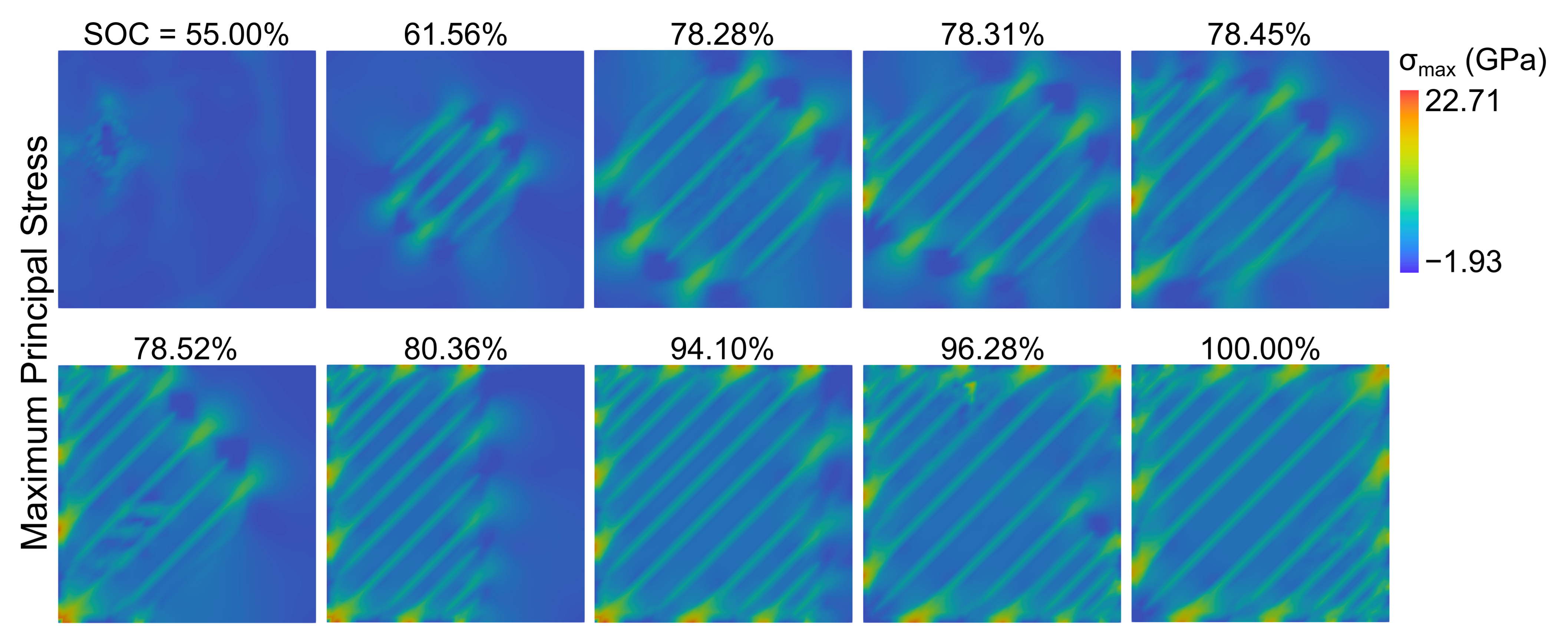
Fig. 10 shows the maximum principal stresses evolving in Li2xMn2O4 electrode during the galvanostatic discharge half cycle. This stress evolution accompanies the Li-intercalation half cycle described in Fig. 8. At the initial state, , the domain is a stress-free single crystal LiMn2O4. On Li-intercalation, at , compressive stresses accompanying the nucleation of the Li-rich Li2Mn2O4 phase are observed in the electrode. It is interesting to note that tensile stresses of GPa are observed at the twin interfaces that separate the tetragonal lattice variants. These twin interfaces theoretically are exactly compatible interfaces that have no lattice misfit. However, in our diffuse interface modeling approach, we introduce regularization terms (i.e., gradient energy terms ) that penalize a change in strain values. This penalty contributes to the finite stresses at the twin interface. Additionally, non-zero stresses are observed at the LiMn2O4/Li2Mn2O4 phase boundary. None of the tetragonal variants of Li2Mn2O4 fit compatibly with the cubic LiMn2O4 lattices. Consequently a finely twinned microstructure, comprising two variants with , forms to minimize the misfit strains at the LiMn2O4/Li2Mn2O4. Despite the energy-minimizing deformation, finite elastic energy is stored in the phase boundary and manifests as stresses during intercalation.
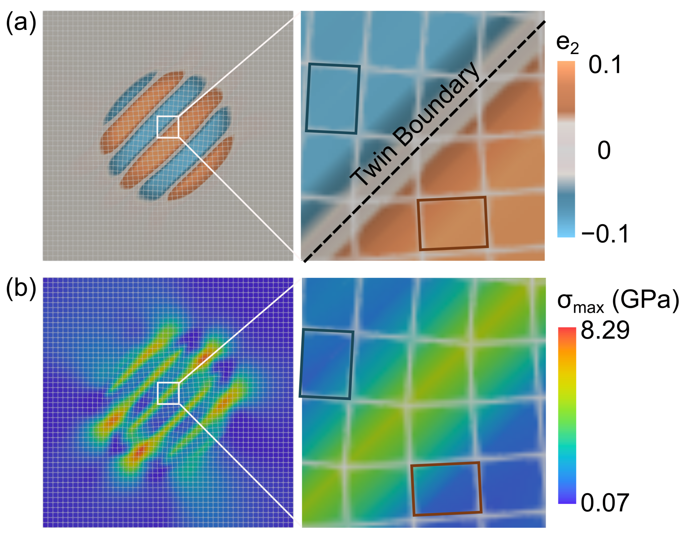
Let us take a closer look at the stress state at , see Fig. 11. We highlight the cubic-to-tetragonal structural transformation of lattices in 2D using a distorted mesh grid. The undeformed square cells correspond to the Li-poor phase and the deformed rectangular cells correspond to the Li-rich phase. The different orientations of the rectangular cells represent the two lattice variants of the Li2Mn2O4 phase. Note that this structural transformation is accompanied by a volume change and lattice strains that contribute to elastic stresses in the domain. In addition to tensile stresses along the twin boundaries, we note stress concentrations at the LiMn2O4 / Li2Mn2O4 interface. These stresses correspond to the lattice mismatch between the cubic and tetragonal phases of the intercalation compound, and the tensile/compressive stresses depend on the lattice orientations at the phase boundary, see Fig. 11(b).
The LiMn2O4 / Li2Mn2O4 phase boundary is elastically stressed, see Fig. 10, and this stressed interface moves through the electrode particle during charge/discharge processes. In experimental literature (Erichsen et al., 2020), this stressed interface is shown to nucleate dislocations and microcracks, that lead to eventual failure of the materials. In these experiments, the dislocations and microcrackings were observed in the proximity of the phase boundary, that is consistent with the stress distribution we observe in our simulation, see Fig. 10. Additionally, in our calculations, this stressed interface interacts with the fixed domain boundaries and contributes to increased stresses at the particle surfaces, see Fig. 10 at . These simulations provide quantitative insights into stress distributions in symmetry-lowering phase transformation materials and serve as a design tool for intercalation materials.
7 Discussion
We derive a thermodynamically-consistent theory that predicts the symmetry-lowering lattice transformations in first-order phase change materials. In this theory, we use the Cauchy-Born rule and the principle of virtual power to develop a multiscale modeling framework that couples finite deformation of lattices at the atomic level with the diffusion of guest species (e.g., intercalating ions) at the continuum level. We applied this theoretical framework to intercalation materials, specifically to a spinel electrode Li1-2Mn2O4, and analyzed the interplay between Li-diffusion and lattice transformation during electrochemical half cycling. The theoretical predictions provide fundamental insights into microstructural evolution pathways in Li1-2Mn2O4 and are consistent with the experimentally imaged HRTEM micrographs in Li2Mn2O4 (Erichsen et al., 2020). Additionally, our simulations predict how individual lattice variants rotate and shear during phase transformations and how they collectively generate elastic stresses at the phase boundary. These insights indicate potential origins of structural decay in Li2Mn2O4 (e.g., microcracking, dislocation nucleation) reported in the literature. In the remainder of this section, we discuss the limiting features of our model and then highlight its potential application for materials design.
Two features of our work limit the comparisons we can make with experimental observations of twinned microstructures in Li2Mn2O4. First, we simplify the form of gradient energy contributions and evolution kinetics by assuming isotropic material constants. For example, we consider a scalar form of the gradient energy coefficients and that penalizes a change in composition or strain variable irrespective of the orientation of the interfaces. Furthermore, to prevent overfitting of the model parameters we do not penalize changes in strain components or the mixed terms. These gradient energy contributions could be important to describe the geometric features of twinned microstructures (e.g., orientation of the phase boundary, volume fraction of the twinned domains) and we will account for these energy terms in our future work. Despite these simplifications, our modeling predictions on twin interface orientations and the nucleation and growth of the lamellar microstructural pattern exhibit a surprisingly favorable comparison with the experimental observations.
Second, due to the nonlinearity and higher-order derivatives involved in the problem, we restrict ourselves to 2D finite element computations. This dimensional reduction simplifies the form of the free energy functional and we primarily describe the energy landscape using the strain variant as the order parameter. This 2D model phenomenologically describes the nucleation and growth of twinned domains in Li2Mn2O4 and predicts principal stresses in 2D at the phase boundary. Individual lattices in bulk Li2Mn2O4, however, rotate and shear in 3D space to minimize the misfit strains at the phase boundary. Computing these microstructural patterns in a 3D finite element framework is necessary to conclusively interpret microstructural evolution pathways and chemo-mechanically coupled stresses in Li2Mn2O4. Extending our model to 3D not only presents a computational challenge, but it is also important to derive the coefficients of higher-order energy terms (e.g., nonlinear elastic energy and anisotropic gradient energy terms) using first-principle calculations (Zhang et al., 2023) and/or careful experimentation. Keeping these limiting conditions in mind, we next discuss the strengths of our diffusion-deformation model and highlight its potential applications.
The key feature of our model is that we derive a thermodynamically-consistent diffusion-deformation theory using the virtual-power approach and the second law of thermodynamics, without specifying, apriori, the form of the free energy function. Through this approach we derive the governing equations based on classical thermodynamic arguments, which differs from other models derived using variational approaches. We numerically solve this model using mixed-type finite element methods based on Lagrange multipliers and implement our framework in an open-source MOOSE platform. Using this model, we predict the interplay between higher-order diffusion terms and nonlinear strain gradient elasticity in Li2Mn2O4 with electrochemical boundary conditions. Unlike earlier phase field models that describe phase transformation in intercalation materials as a function of composition alone Nadkarni et al. (2019); Zhang and Kamlah (2019), our model predicts the coupled interplay between Li-composition and finite lattice deformation and provides quantitative insights into the nucleation and growth of twinned microstructures and stress field distributions during galvanostatic cycling. These insights will play a crucial role in crystallographically designing intercalation materials and mitigating structural degradation (Balakrishna, 2022; Zhang and Balakrishna, 2023; Van der Ven et al., 2023). More broadly, the modeling framework is applicable to describe lattice deformations in other first-order phase transformation materials, such as shape-memory alloys, multicomponent structural materials (Chien et al., 1998; Krogstad et al., 2011) and, 2D layered nanoelectronic materials (Rossnagel, 2010).
8 Conclusions
We derive a thermodynamically consistent theory that couples the diffusion of a guest species at the continuum scale with finite deformation of host lattices at the atomic scale. We adapt this diffusion-deformation theory for symmetry-lowering intercalation materials, such as Li2Mn2O4, and predict the delicate interplay between Li-diffusion and lattice deformation during a galvanostatic insertion half cycle. The present findings contribute to a multiscale understanding of how lattice deformations, in addition to composition phase separation, affect microstructural evolution pathways. Specifically, in Li2Mn2O4, we find that the tetragonal lattice variants nucleate independently in the electrode particle and form compatible twins during phase transformation. These twinned microstructures evolve—by adapting domain thickness and orientation—to lower the misfit strains at the phase boundaries. Our findings quantitatively estimate stress field concentrations in a typical Li2Mn2O4 electrode during a discharge half cycle and suggest a possible mechanism for structural degradation in Li2Mn2O4. More generally, our work establishes a theoretical framework that rigorously couples a Cahn-Hilliard type of diffusion with nonlinear gradient elasticity theory. This framework would be applicable to other symmetry-lowering first-order phase transformation materials beyond intercalation compounds.
Acknowledgments
T. Zhang, D. Zhang, and A. Renuka Balakrishna acknowledge funding from the Air Force Fiscal Year 2023 Young Investigator Research Program (YIP), United States under Grant No. FOA-AFRL-AFOSR-2022-0005. The authors acknowledge the Center for Advanced Research Computing at the University of Southern California and the Center for Scientific Computing at University of California, Santa Barbara for providing resources that contributed to the research results reported in this paper. We thank Dr. Shiva Rudraraju (University of Wisconsin-Madison) for valuable discussions on the project.
Appendix Appendix A Deriving the macroscopic force balance
We rewrite Eq. (18) using index notation:
| (97) | |||||
Integrating Eq. (97) by parts yields
| (98) | |||||
Applying integration by parts again in Eq. (98) but only to Integral A, and using normal gradient operator ()), we obtain
| (99) | |||||
Expanding Integral B of Eq. (99) using surface gradient operator ()) yields
| (100) | |||||
Next, expanding Integral C of Eq. (99) we obtain
| (101) | |||||
Using the following integral identity (Toupin, 1962)
| (104) |
which holds for any smooth tensor field … defined at points of a smooth surface with boundary curve , we expand Integral E as:
| (105) |
Here . are components of the second fundamental form of a smooth part of the boundary and the vector , where is the unit tangent to the curve . By combining Eqs. (99), (101), (102) and (105), we arrive at the index form of macroscopic force balance in section 2.5.1:
| (106) | |||||
The resulting mechanical boundary conditions are given by:
| (107) |
The local macroscopic force balance is given as:
| (108) |
Next, we write the tensor form of Eq. (106) in section 2.5.1 as:
| (109) | |||||
The mechanical boundary conditions are given by:
| (110) |
and the local macroscopic force balance is:
| (111) |
Recall from Eq. (2.7) of the main text, the symmetry condition for the third-order stress tensor can be written as . By combining the symmetry constraint of with Eqs. (100), (103), and (106), we derive the final index notation for the macroscopic force balance as follows:
| (112) | |||||
The index notation representing the local macroscopic force balance remains consistent with Eq. (108). However, the mechanical boundary conditions are derived in the following manner:
| (113) |
Appendix Appendix B Implementing the galvanostatic (dis-)charge condition
Using the relationships and we write the galvanostatic condition in Eq. (68) as follows:
| (116) |
In Eq. (116) the dimensionless global flux is applied on the corresponding dimensionless reactive boundaries . The dimensionless flux is given by:
| (117) |
in which, . Substituting Eq. (117) into Eq. (116) and accounting for active surface areas, we obtain
| (118) |
Here, and we relabel the integrals as:
| (119) |
Here, we consider as a positive solution in order to compute the voltage drop . Please note that the value of is computed and substituted into the Bulter-Volmer equation at every time step in our calculations.
Appendix Appendix C Determining the multiwell potential
First, the chemical potential is related to the open circuit voltage by
| (121) |
Following (Zhang and Kamlah, 2021) we write the chemical potential as
| (124) |
in which and are the binodal concentrations that are found by constructing a common tangent to the multiwell potential curve (Maxwell construction).
Using Eqs. (121) and (124), we fit the OCV to the experimental data (Thackeray et al., 1983) and derive the unknown parameters. We obtain a good fit with the experimental OCV with , and . This ensures that phase segregation occurs at the two binodal concentrations and with the Maxwell construction given by
| (125) |
Appendix Appendix D Symbols
We summarize all symbols used in our work in Table LABEL:T2 below.
| Symbol | Description | Unit |
| The reference body | [/] | |
| Surface of the reference body | [/] | |
| Arbitrary part of the reference body | [/] | |
| Surface of arbitrary part of the reference body | [/] | |
| Smooth boundary edge | [/] | |
| Species concentration in the reference configuration | [] | |
| Maximum reference species concentration | [] | |
| Characteristic length | [] | |
| Time | [] | |
| Diffusion coefficient | [] | |
| Gas constant | [] | |
| Avogadro constant | [] | |
| Reference temperature | [] | |
| Temperature | [] | |
| Elastic constants | [Pa] | |
| Deviatoric modulus | [Pa] | |
| Bulk modulus | [Pa] | |
| Shear modulus | [Pa] | |
| Nonlinear elastic constants | [Pa] | |
| Volume change | [/] | |
| Volume fraction | [/] | |
| Current density | [] | |
| Exchange current density | [] | |
| Reaction rate constant | [] | |
| Electron-transfer symmetry factor | [/] | |
| Faraday constant | [] | |
| Global flux | [] | |
| Dissipation density | [] | |
| Coefficients representing the weight of enthalpy | [/] | |
| Chemical potential in the electrolyte | [] | |
| Reference chemical potential | [] | |
| Chemical potential in the reference configuration | [] | |
| Surface overpotential | [V] | |
| Damköhler number | [/] | |
| Voltage drop | [V] | |
| Bulk free energy density | [] | |
| Gradient energy density | [] | |
| Concentration gradient energy coefficient | [] | |
| Strain gradient energy coefficient | [] | |
| External power | ||
| Internal power power | ||
| Strain measures | [/] | |
| Open circuit voltage | [V] | |
| Gradient operator | [] | |
| Normal gradient operator | [1/m] | |
| Surface gradient operator | [1/m] | |
| Material points | [] | |
| Mapping from material to spatial frame | [] | |
| Vector microscopic force | [] | |
| Displacement | [] | |
| Species flux in the reference configuration | [] | |
| Surface traction | [Pa] | |
| Surface moment | [] | |
| Line force | [] | |
| Body force | [] | |
| Vector | [/] | |
| Lattice vector | [/] | |
| Deformation tensor | [/] | |
| Rotation tensor | [/] | |
| Twin plane direction | [/] | |
| Scalar microscopic traction | [] | |
| Scalar microscopic force | [] | |
| () | Second order unit tensor | [/] |
| Deformation gradient | [/] | |
| First Piola-Kirchhoff stress tensor | [Pa] | |
| Third-order stress tensor | [] | |
| Spontaneous strain | [/] | |
| Lagrange multipliers | [Pa] | |
| Mobility tensor | [] |
References
- Ahluwalia et al. (2006) Ahluwalia, R., Lookman, T., Saxena, A., 2006. Dynamic strain loading of cubic to tetragonal martensites. Acta materialia 54, 2109–2120.
- Anand (2012) Anand, L., 2012. A Cahn–Hilliard-type theory for species diffusion coupled with large elastic–plastic deformations. Journal of the Mechanics and Physics of Solids 60, 1983–2002.
- Bai et al. (2011) Bai, P., Cogswell, D.A., Bazant, M.Z., 2011. Suppression of phase separation in LiFePO4 nanoparticles during battery discharge. Nano Letters 11, 4890–4896.
- Balakrishna (2022) Balakrishna, A.R., 2022. Crystallographic design of intercalation materials. Journal of Electrochemical Energy Conversion and Storage 19, 040802.
- Balakrishna and Carter (2018) Balakrishna, A.R., Carter, W.C., 2018. Combining phase-field crystal methods with a Cahn-Hilliard model for binary alloys. Physical Review E 97, 043304.
- Balakrishna et al. (2019) Balakrishna, A.R., Chiang, Y.M., Carter, W.C., 2019. Phase-field model for diffusion-induced grain boundary migration: An application to battery electrodes. Physical Review Materials 3, 065404.
- Ball and James (1987) Ball, J.M., James, R.D., 1987. Fine phase mixtures as minimizers of energy. Archive for Rational Mechanics and Analysis 100, 13–52.
- Barsch and Krumhansl (1984) Barsch, G., Krumhansl, J., 1984. Twin boundaries in ferroelastic media without interface dislocations. Physical Review Letters 53, 1069.
- Bhattacharya (2003) Bhattacharya, K., 2003. Microstructure of martensite: why it forms and how it gives rise to the shape-memory effect. volume 2. Oxford University Press.
- Chien et al. (1998) Chien, F., Ubic, F., Prakash, V., Heuer, A., 1998. Stress-induced martensitic transformation and ferroelastic deformation adjacent microhardness indents in tetragonal zirconia single crystals. Acta materialia 46, 2151–2171.
- Christensen and Newman (2006) Christensen, J., Newman, J., 2006. A mathematical model of stress generation and fracture in lithium manganese oxide. Journal of The Electrochemical Society 153, A1019.
- Cogswell and Bazant (2012) Cogswell, D.A., Bazant, M.Z., 2012. Coherency strain and the kinetics of phase separation in LiFePO4 nanoparticles. ACS Nano 6, 2215–2225.
- Cowley (1976) Cowley, R., 1976. Acoustic phonon instabilities and structural phase transitions. Physical Review B 13, 4877.
- Di Leo et al. (2014) Di Leo, C.V., Rejovitzky, E., Anand, L., 2014. A Cahn–Hilliard-type phase-field theory for species diffusion coupled with large elastic deformations: application to phase-separating Li-ion electrode materials. Journal of the Mechanics and Physics of Solids 70, 1–29.
- Erichsen et al. (2020) Erichsen, T., Pfeiffer, B., Roddatis, V., Volkert, C.A., 2020. Tracking the diffusion-controlled lithiation reaction of by In Situ TEM. ACS Applied Energy Materials 3, 5405–5414.
- Ericksen (2008) Ericksen, J., 2008. On the cauchy—born rule. Mathematics and mechanics of solids 13, 199–220.
- Ganser et al. (2019) Ganser, M., Hildebrand, F.E., Klinsmann, M., Hanauer, M., Kamlah, M., McMeeking, R.M., 2019. An extended formulation of butler-volmer electrochemical reaction kinetics including the influence of mechanics. Journal of The Electrochemical Society 166, H167.
- Gaston et al. (2009) Gaston, D., Newman, C., Hansen, G., Lebrun-Grandie, D., 2009. Moose: A parallel computational framework for coupled systems of nonlinear equations. Nuclear Engineering and Design 239, 1768–1778.
- Gurtin (1996) Gurtin, M.E., 1996. Generalized Ginzburg-Landau and Cahn-Hilliard equations based on a microforce balance. Physica D: Nonlinear Phenomena 92, 178–192.
- Gurtin (2002) Gurtin, M.E., 2002. A gradient theory of single-crystal viscoplasticity that accounts for geometrically necessary dislocations. Journal of the Mechanics and Physics of Solids 50, 5–32.
- Han et al. (2004) Han, B., Van der Ven, A., Morgan, D., Ceder, G., 2004. Electrochemical modeling of intercalation processes with phase field models. Electrochimica Acta 49, 4691–4699.
- Hörmann and Groß (2019) Hörmann, N.G., Groß, A., 2019. Phase field parameters for battery compounds from first-principles calculations. Physical Review Materials 3, 055401.
- Krogstad et al. (2011) Krogstad, J.A., Krämer, S., Lipkin, D.M., Johnson, C.A., Mitchell, D.R., Cairney, J.M., Levi, C.G., 2011. Phase stability of -zirconia-based thermal barrier coatings: mechanistic insights. Journal of the American Ceramic Society 94, s168–s177.
- Luo et al. (2020) Luo, F., Wei, C., Zhang, C., Gao, H., Niu, J., Ma, W., Peng, Z., Bai, Y., Zhang, Z., 2020. Operando x-ray diffraction analysis of the degradation mechanisms of a spinel cathode in different voltage windows. Journal of Energy Chemistry 44, 138–146.
- Mykhaylov et al. (2019) Mykhaylov, M., Ganser, M., Klinsmann, M., Hildebrand, F., Guz, I., McMeeking, R., 2019. An elementary 1-dimensional model for a solid state lithium-ion battery with a single ion conductor electrolyte and a lithium metal negative electrode. Journal of the Mechanics and Physics of Solids 123, 207–221.
- Nadkarni et al. (2019) Nadkarni, N., Zhou, T., Fraggedakis, D., Gao, T., Bazant, M.Z., 2019. Modeling the metal–insulator phase transition in LixCoO2 for energy and information storage. Advanced Functional Materials , 1902821.
- Ombrini et al. (2023) Ombrini, P., Bazant, M.Z., Wagemaker, M., Vasileiadis, A., 2023. Thermodynamics of multi-sublattice battery active materials: from an extended regular solution theory to a phase-field model of . npj Computational Materials 9, 148.
- Padhi et al. (1997) Padhi, K.A., Nanjundaswamy, S.K., Goodenough, B.J., 1997. Phospho-olivines as positive-electrode materials for rechargeable lithium batteries. Journal of the electrochemical society 144, 1188.
- Ramogayana (2020) Ramogayana, B., 2020. Lithium manganese oxide (LiMn2O4) spinel surfaces and their interaction with the electrolyte content. Ph.D. thesis.
- Redlich and Kister (1948) Redlich, O., Kister, A., 1948. Activity coefficient model. Ind Eng Chem 24, 345–52.
- Rossnagel (2010) Rossnagel, K., 2010. Suppression and emergence of charge-density waves at the surfaces of layered and by in situ rb deposition. New Journal of Physics 12, 125018.
- Rudraraju et al. (2014) Rudraraju, S., Van der Ven, A., Garikipati, K., 2014. Three-dimensional isogeometric solutions to general boundary value problems of toupin’s gradient elasticity theory at finite strains. Computer Methods in Applied Mechanics and Engineering 278, 705–728.
- Rudraraju et al. (2016) Rudraraju, S., Van der Ven, A., Garikipati, K., 2016. Mechanochemical spinodal decomposition: a phenomenological theory of phase transformations in multi-component, crystalline solids. npj Computational Materials 2, 1–9.
- Santos et al. (2023) Santos, D.A., Rezaei, S., Zhang, D., Luo, Y., Lin, B., Balakrishna, A.R., Xu, B.X., Banerjee, S., 2023. Chemistry–mechanics–geometry coupling in positive electrode materials: a scale-bridging perspective for mitigating degradation in lithium-ion batteries through materials design. Chemical Science 14, 458–484.
- Schofield et al. (2022) Schofield, P., Luo, Y., Zhang, D., Zaheer, W., Santos, D., Agbeworvi, G., Ponis, J.D., Handy, J.V., Andrews, J.L., Braham, E.J., et al., 2022. Doping-induced pre-transformation to extend solid-solution regimes in li-ion batteries. ACS Energy Letters 7, 3286–3292.
- Shchyglo et al. (2012) Shchyglo, O., Salman, U., Finel, A., 2012. Martensitic phase transformations in ni–ti-based shape memory alloys: The landau theory. Acta materialia 60, 6784–6792.
- Shu et al. (1999) Shu, J.Y., King, W.E., Fleck, N.A., 1999. Finite elements for materials with strain gradient effects. International Journal for Numerical Methods in Engineering 44, 373–391.
- Tang et al. (2010) Tang, M., Carter, W.C., Belak, J.F., Chiang, Y.M., 2010. Modeling the competing phase transition pathways in nanoscale olivine electrodes. Electrochimica Acta 56, 969–976.
- Thackeray et al. (1983) Thackeray, M.M., David, W.I., Bruce, P.G., Goodenough, J.B., 1983. Lithium insertion into manganese spinels. Materials Research Bulletin 18, 461–472.
- Thomas and Van der Ven (2017) Thomas, J.C., Van der Ven, A., 2017. The exploration of nonlinear elasticity and its efficient parameterization for crystalline materials. Journal of the Mechanics and Physics of Solids 107, 76–95.
- Toupin (1962) Toupin, R., 1962. Elastic materials with couple-stresses. Archive for rational mechanics and analysis 11, 385–414.
- Van der Ven et al. (2023) Van der Ven, A., McMeeking, R.M., Clément, R.J., Garikipati, K., 2023. Ferroelastic toughening: Can it solve the mechanics challenges of solid electrolytes? Current Opinion in Solid State and Materials Science 27, 101056.
- Wan et al. (2016) Wan, J., Lacey, S.D., Dai, J., Bao, W., Fuhrer, M.S., Hu, L., 2016. Tuning two-dimensional nanomaterials by intercalation: materials, properties and applications. Chemical Society Reviews 45, 6742–6765.
- Whittingham (1978) Whittingham, M.S., 1978. Chemistry of intercalation compounds: Metal guests in chalcogenide hosts. Progress in Solid State Chemistry 12, 41–99.
- Zhang and Balakrishna (2023) Zhang, D., Balakrishna, A.R., 2023. Designing shape-memory-like microstructures in intercalation materials. Acta Materialia , 118879.
- Zhang et al. (2021) Zhang, D., Sheth, J., Sheldon, B.W., Balakrishna, A.R., 2021. Film strains enhance the reversible cycling of intercalation electrodes. Journal of the Mechanics and Physics of Solids 155, 104551.
- Zhang and Kamlah (2018) Zhang, T., Kamlah, M., 2018. Sodium ion batteries particles: Phase-field modeling with coupling of Cahn-hilliard equation and finite deformation elasticity. Journal of The Electrochemical Society 165, A1997.
- Zhang and Kamlah (2019) Zhang, T., Kamlah, M., 2019. Phase-field modeling of the particle size and average concentration dependent miscibility gap in nanoparticles of LixMn2O4, LixFePO4, and NaxFePO4 during insertion. Electrochimica Acta 298, 31–42.
- Zhang and Kamlah (2020) Zhang, T., Kamlah, M., 2020. Mechanically coupled phase-field modeling of microstructure evolution in sodium ion batteries particles of NaxFePO4. Journal of The Electrochemical Society 167, 020508.
- Zhang and Kamlah (2021) Zhang, T., Kamlah, M., 2021. Microstructure evolution and intermediate phase-induced varying solubility limits and stress reduction behavior in sodium ion batteries particles of NaxFePO4 (). Journal of Power Sources 483, 229187.
- Zhang et al. (2023) Zhang, T., Sotoudeh, M., Groß, A., McMeeking, R.M., Kamlah, M., 2023. 3D microstructure evolution in NaxFePO4 storage particles for sodium-ion batteries. Journal of Power Sources 565, 232902.
- Zhang et al. (2007) Zhang, X., Shyy, W., Sastry, A.M., 2007. Numerical simulation of intercalation-induced stress in Li-ion battery electrode particles. Journal of the Electrochemical Society 154, A910.