Counting Phases and Faces Using
Bayesian Thermodynamic Integration

Posterior distribution $\mathbb{P}(\textbf{t}|s)$ works as a sort of “probabilistic thermometer”: it looks at a microstate $s$ and gives a probabilistic forecast of external parameters (for example temperature) at which this microstate was generated.

By definition of the problem, it is possible to sample from $\mathbb{P}(s|\textbf{t})$, giving pairs

sampled from joint distribution, where $\mathbb{P}(\textbf{t})$ is chosen to be uniform in some compact domain. These samples can be used to fit parametric family of distributions $\mathbb{P}_{\theta}(\textbf{t}|s)$ to approximate posterior $\mathbb{P}(\textbf{t}|s)$. Here $\theta$ are the parameters of the family of distribution, which could be obtained by maximizing likelihood of true external parameters $\textbf{t}_{i}$ given $s_{i}$ over all our samples or equivalently by minimizing negative log-likelihood

Minimization of the log-likelihood (7) is equivalent to minimization of the KL divergence between the distribution of target labels and the predicted distribution

where $s(\textbf{t}^{\prime})$ is a microstate of the physical model sampled from the conditional distribution $\mathbb{P}(s|\textbf{t}^{\prime})$. If labels are considered hard, the target distribution is $\mathbb{P}_{\text{target}}(\textbf{t}|\textbf{t}^{\prime})=\delta(\textbf{t}-\textbf{t}^{\prime})$. In order to avoid divergences, it is convenient to use a smoothened distribution

instead. Here $C$ is the normalizing constant, it is obtained by integrating over the domain of interest in the space of macroscopic parameters. The standard deviation $\sigma$ is defined to be equal to the mean distance from a point $t$ in the training dataset to its K-th nearest neighbor.

The resulting parametric distribution can be used as input of formula (6) in order to get an approximation of the Fisher metric. However, this approach has two important drawbacks.

First, in order to obtain a decent approximation the parametric family $\mathbb{P}_{\theta}$ should be flexible enough, implying a large number of parameters $\theta$. However, if $\dim(\theta)>>N$, i.e. if the number of parameters is much larger than the number of examples in the training set, the problem of overfitting arises.

Second, the Fisher metric depends on the derivative of the approximated function, and derivatives of approximated functions are typically much noisier than the functions themselves. As a result, without additional efforts to smooth the posterior distribution, approximation (6) turns out to be too noisy to be useful in practice.

In order to resolve the first problem we artificially augment the training set. Instead of using a single microstate $s$ as an input for the prediction of external parameters t we use a randomly shuffled tuple of $K$ microstates $s_{1},\dots,s_{K}$ generated at external parameters close to t. That is to say, start with a set of $N$ training pairs $(s_{i},\textbf{t}_{i})$, for each $\textbf{t}_{i}$ choose $K$ values $\textbf{t}_{j}$ with the smallest distance $||\textbf{t}_{i}-\textbf{t}_{j}||$, form a randomly shuffled tuple out of the corresponding microstates, and use the set $(\{s_{i,1},\dots,s_{i,K}\},\textbf{t}_{i})$ as a training set, so that instead of $\mathbb{P}_{\theta}(\textbf{t}_{i}|s_{i})$ we are now training the model to predict $\mathbb{P}_{\theta}(\textbf{t}_{i}|s_{i,1},\dots,s_{i,K})$. This trick allows to increase the size of the training set by a factor $K!$ without generating any new microstates. The drawback is that the resolution with respect to t decreases with growing $K$. However, this decrease is much slower, then the factorial growth of the size of the training set.

The resulting target distribution $\mathbb{P}_{\text{target}}(\textbf{t}|\textbf{t}^{\prime})$ is obtained by averaging target distributions (10) over the $K$ nearest neighbours

In order to resolve the second issue outlined above we approximate the posterior distribution with a distribution from the exponential family parametrized by convex function, as described in the next section.

We know that Fisher metric is a positive-definite matrix $\delta\textbf{t}^{T}G(\textbf{t})\delta\textbf{t}\geq 0\ \ \forall\ \delta\textbf{t}$. The main idea of our approach is to approximate this positive-definite matrix by the Hessian of a convex function. Note that this means that if $\dim(\textbf{t})=1$, i.e. if there is a single scalar external macroscopic parameter, then this approximation is exact.

More precisely, we approximate the posterior distribution as a function of external parameters by a distribution from the so-called exponential family of distributions. It is instructive to introduce this family in a following way. Suppose for each value of t we fix average values of some macroscopic observables $\int\mathbb{P}(s|\textbf{t})f(s)ds=\Gamma(\textbf{t})$. We are interested in a probability distribution $\mathbb{P}(s)$, which maximizes entropy

while respecting this constraint. Maximizing the functional

where t, and $\lambda_{0}$ are Lagrange multipliers, gives the exponential family distributions of the form

where the normalization factor

is known as “the partition function” in equilibrium statistical mechanics.

For distributions from exponential family Fisher metric reduces to Hessian of the logarithm of the partition function

while its first derivatives are the mean values of the function $f(s)$ and are known as “thermodynamic forces”

Fisher metric tensor is known to be positive-definite, and thus the function $\log Z(\textbf{t})$ is convex.

Now, in order to solve the problem of approximating the derivatives of the posterior distribution $\mathbb{P}(\textbf{t}|s)$, we want to find a function $Z_{w}(\textbf{t})$, depending on some set of parameters $w$ which is, on the one hand, convex, and on the other hand, such that the Jensen-Shannon divergence between the approximate posterior $\mathbb{P}_{\theta}(\textbf{t}|s)$ and the posterior distribution generated from the exponential family with partition function $Z_{w}(\textbf{t})$ is minimized.

If our prior is uniform then exponential-family posterior distribution takes the form

Function $f(s)$ is unknown, but since we use a tuple of microstates to estimate a single posterior, we replace $f(s)$ by its expectation (17),

To find parameters $w$ we minimize Jensen-Shannon divergence between posterior $\mathbb{P}_{\theta}(\textbf{t}|s)$ predicted using maximum likelihood and posterior $\mathbb{P}_{w}(\textbf{t}|s)$ with $f(s)$ replaced by the gradient of the partition function

The resulting approximation for the Fisher metric is

We summarize the procedure described in this section by two algorithms outlined below, the first one generates the training dataset (1), the second one finds the approximations for the partition function and the Fisher metric (2).

In this section we test whether our approach is capable of reconstructing thermodynamic functions for an equilibrium statistical mechanics model in which the distribution of microstates belongs to the exponential family. We consider a 2D Ising model ising1925beitrag , which is an archetypal model of phase transitions in statistical mechanics. A microstate of this model is a set $s$ of spin variables $s_{i}=\pm 1$ defined on each vertex of a square lattice of size $L\times L$. At equilibrium probability distribution over the space of microstates is

where $H$ and $T=1/\beta$ are external parameters called magnetic field and temperature, respectively, the first sum is over all edges of the lattice, and $Z(H,T)$ is a normalization parameter known as a partition function:

This model is exactly solvable for $H=0$ onsager1944crystal ; kac1952combinatorial ; baxter1978399th . In particular, it is known that at $T_{\text{cr}}=\frac{2}{\log(1+\sqrt{2})}\approx 2.269$ a transition occurs between the high-temperature disordered state, where spin variables are on average equal zero, and the low-temperature ordered state in which average value of spin becomes distinct from zero. For general values of $H\neq 0$ the likelihood function (22) is intractable.

Our dataset consists of $N=540000$ samples of spin configurations on the square lattice of size $L\times L=128\times 128$ with periodic boundary conditions. We consider the parameter ranges $T\in[T_{\min},T_{\max}]=[1,5],H\in[H_{\min},H_{\max}]=[-2,2]$ similar to the ranges used in (Walker, 2019). Point $(T,H)$ is sampled uniformly from this rectangle, and then a sample spin configuration is created for these values of temperature and external field by starting with a random initial condition and equilibrating is with Glauber (one-spin Metropolis) dynamics for $10^{4}\times 128\times 128\approx 1.64\times 10^{8}$ iterations. We represent spin configuration as a single-channel image with values $+1$ and $-1$. When constructing target probability distributions we choose $\sigma=\frac{1}{50}$ and set the discretization $\mathcal{D}$ of the square $[T_{\min},T_{\max}]\times[H_{\min},H_{\max}]=[1,5]\times[-2,2]$ to be a uniform grid with $L\times L=128\times 128$ grid cells.

Image-to-image network with U²-Net architecture qin2020u2 is used to approximate posterior $\mathbb{P}_{\theta}(\textbf{t}|s)$. The network takes as input a bundle of $K_{\text{bundle}}$ images concatenated across channel dimension and outputs a categorical distribution representing density values in discrete grid points. For simplicity we choose the discretization $\mathcal{D}$ to be of the same spatial dimensions as the input image. For all our numerical experiments the training was performed on a single Nvidia-HGX compute node with 8 A100 GPUs. We trained U²-Net using Adam optimizer with learning rate $0.00001$ and batch size of $2048$ for $N_{\text{U2Net steps}}=20000$ gradient update steps. In all our experiments the training set consists of 80% of samples and the other 20% are used for testing.

Bundle augmentation. To explore how test loss depends on the bundle size $K_{\text{bundle}}$, which determines the number of microstates used to evaluate a single posterior distribution, we performed four different training runs with $K_{\text{bundle}}\in\{1,2,3,8\}$. The results are shown in 2. For $K_{\text{bundle}}=1$, we observed overfitting after about the 12000th training iteration. However, even with $K_{\text{bundle}}=2$, overfitting is significantly reduced and continues to decrease at large values of $K_{\text{bundle}}$. The downside of this approach is that the effective grid resolution of the posterior distribution decreases with growing $K_{\text{bundle}}$ as

where $N$ is the dataset size. In what follows, we set $K_{\text{bundle}}=4$. Also, since we are using a fully convolutional architecture, increasing the number of input channels by $K_{\text{bundle}}$ times has almost no effect on the overall GPU memory consumption during training.

Free energy approximation. We use Input Convex Neural Network amos2017input architecture to approximate the free energy. The fully connected ICNN has 5 layers with hidden dimension 512. We train network using Adam optimizer with learning rate 0.001.

Reconstructed free energy is shown in 3. The model was able to correctly determine 1st order phase transition line $T<T_{\text{cr}}$ and $H=0$.

Totally asymmetric simple exclusion process (TASEP) is a simple model of 1-dimensional transport phenomena. A microscopic configuration is a set of particles on a 1d lattice respecting the condition that there can be no more than one particle in each lattice cell. Each particle can move to the site to the right of it with probability $pdt$ per time $dt$ provided that it is empty (we put $p=1$ without loss of generality). When complemented with boundary conditions, the TASEP attains a stationary state as time goes to infinity.

One particular case is open boundary conditions, when a particle is added with probability $\alpha dt$ per time $dt$ to the leftmost site provided that it is empty and removed with probability $\beta dt$ per time $dt$ from the rightmost site provided that it is occupied. For this boundary condition the probability distribution is known exactly dehp ; evans_review ; krapivsky_book and it once again takes the form

where microstate $s$ is a concrete sequence of filled and empty cells, and $f(s|\alpha,\beta)$ is some function of $s$ and external parameters $\alpha,\beta$. Importantly, however, the function $f$, which is known exactly for all system sizes $M$ and all values of $s,\alpha,\beta$ does not take the form (14). TASEP with free boundaries exhibits a rich phase behavior: for large system sizes three distinct phases - the low-density phase, the high-density phase and the maximal current phase are possible depending on the values of $\alpha,\beta$, and the asymptotic ”free energy” which is defined as

and coincides with average flow per unit time, equals

where the first, second and third cases correspond to maximal current, high density and low density cases, respectively.

We generate a dataset of $N=150000$ stationary TASEP configurations on a 1d lattice with $M=16384$ sites. The rates $\alpha(\beta)$ of adding (removing) particles at the left(right) boundary are sampled from the uniform prior distribution over a square $[0,1]\times[0,1]$. To reach the stationary state we start from a random initial condition and perform $N_{\text{steps}}=2\times 10^{9}\approx 8M^{2}$ move attempts, which is known to be enough to achieve the stationary state except for the narrow vicinity of the transition line $\alpha=\beta<1/2$ between high-density and low-density phases (in this case the stationary state has a slowly diffusing front of a shock wave in it, one needs of order $M^{2}$ move attempts to form the shock but of order $M^{3}$ move attempts for it to diffusively explore all possible positions of the shock).

We reshape 1d lattice with $M=16384$ sites into an image of size $L\times L=128\times 128$ using raster scan ordering. To construct target probability distributions we set $\sigma=\frac{1}{150}$ and define the discretization $\mathcal{D}$ as a uniform grid on $[\alpha_{\min},\alpha_{\max}]\times[\beta_{\min},\beta_{\max}]=[0,1]\times[0,1]$ with $L\times L=128\times 128$ grid cells.

The comparison of the reconstructed free energy and the exact analytical solution is shown in 5.

Consider a synthetic two-parametric statistical mechanics model where microstates are sampled using the StyleGAN v3 generator karras2021alias . Let $z_{1},z_{2}$ and $z_{3}$ be vectors from the latent space of dimension 512. Consider a 2d section of the latent space parameterized by $a$ and $b$ as follows

where $\xi$ is a normally distributed random vector with zero mean and small enough standard deviation (we it to be 1/5 of the standard deviation of the prior standard normal distribution). External parameters $a$ and $b$ lie in the rectangle $[0,1]\times[0,1]$, so that $z(a,b)$ interpolates between three base latent vectors at the corners $z(0,0)=z_{1}$, $z(1,0)=z_{2}$, $z(0,1)=z_{3}$ of the rectangle. By putting latent code $z(a,b)$ into the generator of StyleGAN we can sample images as functions of two external parameters.

For FFHQ dataset we generate dataset of $N=500000$ human faces using StyleGAN at resolution of $1024\times 1024$ and resize it to the resolution $128\times 128$ before feeding it to the U2Net model which approximates posterior distribution on the space of external parameters. Experiment setup was similar to the 2D Ising model.

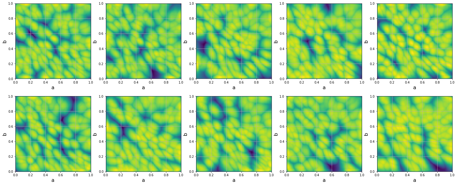
Reconstructed Fisher metric is shown in 7. Unexpectedly, we found two diagonal lines in the components of the Fisher metric, which, from the point of view of statistical mechanics, are signs of second-order phase transitions. If we compare it with the faces presented in 6 and 13 we can observe that phase transition lines correspond to the sharp identity change of generated faces. In the next section we investigate whether this behaviour is determined by the mapping network part of StyleGAN or it depends only on the synthesis network.

Given a latent vector $z$ the StyleGAN v3 generates images in two steps. First, the mapping network is applied to generate a vector (code) in the intermediate latent space $\mathcal{W}$. This latent code in case of the StyleGAN v3 model pretrained on FFHQ dataset is a matrix with shape $16\times 512$ karras2021alias ; karras2020analyzing . Second, this vector is used by the weight demodulation layers of the synthesis network to generate the image itself.

A lot of attention was devoted to the improvement of the synthesis network. The effect of the mapping network on the generated images attracted less attention. To study which network, mapping or synthesis, is responsible for the typical shape of the Fisher metric field of the StyleGAN we introduce another synthetic two-parametric statistical mechanics model where microstates are generated by the mapping network

Similarly to the previous section we generate $N=500000$ intermediate latent code of the shape $16\times 512$ for the same latent vectors $z(a,b)$ and resize it into an image of size $128\times 128$.

As it can be seen from the 9 and 7 Fisher metric fields for image space and for the $\mathcal{W}$ space almost coincide which means that mostly the mapping network defines variability of the generated faces and the synthesis network doesn’t change the distribution of output images. In other words the synthesis network performs almost a bijective transformation of vectors from the intermediate latent space $\mathcal{W}$.

References

- (1) Amari, S.-I., Nagaoka, H. Methods of information geometry, American Mathematical Soc., Providence, RI, 2000.
- (2) Ising, E. Beitrag zur theorie des ferromagnetismus. Zeitschrift für Physik, 31, 253 (1925).
- (3) Onsager, L. Crystal statistics. I. a two-dimensional model with an order-disorder transition. Physical Review, 65, 117 (1944).
- (4) Kac, M. and Ward, J. C. A combinatorial solution of the two-dimensional Ising model. Physical Review, 88, 1332 (1952).
- (5) Baxter, R. J. and Enting, I. G. 399th solution of the Ising model. J. Phys. A: Math. and Gen., 11, 2463 (1978).
- (6) Qin, X., Zhang, Z., Huang, C., Dehghan, M., Zaiane, O. R., and Jagersand, M. U2-net: Going deeper with nested u-structure for salient object detection. Pattern Recognition, 106, 107404 (2020).
- (7) Amos, B., Xu, L., and Kolter, J. Z. Input convex neural networks. In International Conference on Machine Learning, p. 146. (2017).
- (8) Derrida, B., Evans, M. R., Hakim, V., and Pasquier, V. Exact solution of a 1d asymmetric exclusion model using a matrix formulation. J. Phys. A: Math. and Gen., 26, 1493 (1993).
- (9) Blythe, R. A. and Evans, M. R. Nonequilibrium steady states of matrix-product form: a solver’s guide. J. Phys. A: Math. and Gen., 40, R333 (2007).
- (10) Krapivsky, P. L., Redner, S., and Ben-Naim, E. A kinetic view of statistical physics. Cambridge University Press, 2010.
- (11) Karras, T., Aittala, M., Laine, S., Härkönen, E., Hellsten, J., Lehtinen, J., and Aila, T. Alias-free generative adversarial networks. Advances in Neural Information Processing Systems, 34 (2021).
- (12) Karras, T., Laine, S., Aittala, M., Hellsten, J., Lehtinen, J., and Aila, T. Analyzing and improving the image quality of stylegan. In Proceedings of the IEEE/CVF Conference on Computer Vision and Pattern Recognition, pp. 8110 (2020).
- (13) Van Nieuwenburg, E. P., Liu, Y.-H., and Huber, S. D. Learning phase transitions by confusion. Nature Physics, 13, 435 (2017).
- (14) Carrasquilla, J. and Melko, R. G. Machine learning phases of matter. Nature Physics, 13, 431 (2017).
- (15) Rem, B. S., Käming, N., Tarnowski, M., Asteria, L., Fläschner, N., Becker, C., Sengstock, K., and Weitenberg, C. Identifying quantum phase transitions using artificial neural networks on experimental data. Nature Physics, 15, 917 (2019).
- (16) Wang, J., Zhang, W., Hua, T., and Wei, T.-C. Unsupervised learning of topological phase transitions using the Calinski-Harabaz index. Physical Review Research, 3, 013074 (2021).
- (17) Canabarro, A., Fanchini, F. F., Malvezzi, A. L., Pereira, R., and Chaves, R. Unveiling phase transitions with machine learning. Physical Review B, 100, 045129 (2019).
- (18) Jiang, B., Wu, T.-Y., Zheng, C., and Wong, W. H. Learning summary statistic for approximate bayesian computation via deep neural network. Statistica Sinica, p. 1595 (2017).
- (19) Chen, Y., Zhang, D., Gutmann, M., Courville, A., and Zhu, Z. Neural approximate sufficient statistics for implicit models, arXiv:2010.10079.
- (20) Walker, N., Tam, K.-M., and Jarrell, M. Deep learning on the 2-dimensional Ising model to extract the crossover region with a variational autoencoder. Scientific reports, 10, 1 (2020).
- (21) Tran, N.-T., Bui, T.-A., and Cheung, N.-M. Dist-gan: An improved GAN using distance constraints. In Proceedings of the European Conference on Computer Vision (ECCV), p. 370 (2018).
- (22) Novikov, G. S., Panov, M. E., and Oseledets, I. V. Tensor-train density estimation. In Uncertainty in Artificial Intelligence, pp. 1321, PMLR, 2021.
- (23) Zacharov, I., Arslanov, R., Gunin, M., Stefonishin, D., Bykov, A., Pavlov, S., Panarin, O., Maliutin, A., Rykovanov, S., and Fedorov, M. “Zhores”—petaflops supercomputer for data-driven modeling, machine learning and artificial intelligence installed in Skolkovo Institute of Science and Technology. Open Engineering, 9, 512 (2019).
Appendix A Learned posterior distributions for 2D Ising model
Appendix B StyleGAN v3 linear interpolation between three base faces
Appendix C Reconstructed Fisher metrics
Appendix D StyleGAN v3 latent space visualization
D.1 Density-based visualization of the posterior distribution on the space of macroscopic parameters
D.2 Log-density-based visualization of the posterior distribution on the space of macroscopic parameters