Counting Parabolic Double Cosets in Symmetric Groups
Abstract
Billey, Konvalinka, Petersen, Solfstra, and Tenner recently presented a method for counting parabolic double cosets in Coxeter groups, and used it to compute , the number of parabolic double cosets in , for . In this paper, we derive a new formula for and an efficient polynomial time algorithm for evaluating this formula. We use these results to compute for and to prove an asymptotic formula for that was conjectured by Billey et al.
1 Introduction
For a Coxeter system , each subset generates a subgroup of . These subgroups of are called parabolic subgroups. A parabolic double coset in the Coxeter system is a double coset of the form for and . Parabolic double cosets have several properties that make them interesting objects to study. For example, the parabolic double cosets of a finite Coxeter group are rank-symmetric intervals in the Bruhat order on [3], and the poset of presentations of parabolic double cosets gives a boolean complex that retains many properties of the Coxeter complex [6].
The problem of counting parabolic double cosets is considered in [1]. Counting parabolic double cosets is hard because a given parabolic double coset might arise from multiple choices of and . To avoid this problem, Billey, Konvalinka, Petersen, Slofstra, and Tenner take the approach of counting lex-minimal presentations [1]. The lex-minimal presentation of a parabolic double coset is the unique presentation such that is the minimal element of in the Bruhat order and such that is lexicographically minimal among all presentations of . Theorem 4.26 of [1] gives a formula for the number of parabolic double cosets with a given minimal element , for any Coxeter group . In the case of the symmetric group, , summing this formula over all elements of will compute , the total number of distinct parabolic double cosets in . The sequence may be found at [5, A260700]. The values of for have been computed using this method [1]. However, the summation over all elements of limits the number of terms of that can be computed with this approach.
In this paper we restrict our attention to counting parabolic double cosets in . Two ways of depicting parabolic double cosets in are the balls-in-boxes model considered in [1] and two-way contingency tables, which are matrices of nonnegative integers with nonzero row sums and column sums. Diaconis and Gangolli use the balls-in-boxes model to give a bijection between parabolic double cosets in the double quotient and two-way contingency tables with prescribed row sums and column sums [2]. They attribute the idea behind the bijection to Nantel Bergeron. This bijection is also used in [6], where it provides an alternate construction of the two-sided Coxeter complex of in terms of two-way contingency tables.
There are three main results of this paper. The first result is the explicit formula
| (1) |
where the values are generalizations of the Fubini numbers. The second result is an efficient polynomial time algorithm to evaluate this formula, which is used to compute the values of for . These values of are summarized in the appendix. The third result is an asymptotic formula for that proves the following conjecture.
Conjecture 1.1 (Conjecture 1.4 in [1]).
There exists a constant so that
Theorem 1.2.
Conjecture 1.1 holds with constant
We conclude this introduction by outlining the two key ideas behind formula (1). The first idea is to associate each parabolic double coset with a canonical two-way contingency table. In particular, there is a bijection between parabolic double cosets in and two-way contingency tables with sum that are “maximal” (as defined at the end of section 2). This reduces the problem of computing to the problem of counting maximal two-way contingency tables with sum .
Two-way contingency tables have both a restriction on the rows (nonzero row sums) and a restriction on the columns (nonzero column sums). These two restrictions are entangled since any nonzero entry in the table both makes its row sum nonzero and its column sum nonzero. The second idea is to break this entanglement by transforming the problem from counting two-way contingency tables to counting pairs of weak orders (a weak order is a binary relation that is transitive and has no incomparable pairs of elements).
This transformation is applied in sections 3.2 and 3.3 to the problem of counting maximal two-way contingency tables with sum , as well as to the simpler problem of counting all two-way contingency tables with sum . More generally, this transformation is applicable whenever counting two-way contingency tables with a restriction on the locations of nonzero entries, but not on their specific values.
2 Background
In this section, we give an overview of parabolic double cosets in , and describe two ways of depicting presentations of parabolic double cosets in . We will use to denote the th adjacent transposition in (the transposition that swaps and ).
Definition 2.1.
A parabolic subgroup in the symmetric group is a subgroup of generated by a collection of adjacent transpositions in .
Definition 2.2.
A parabolic double coset in the symmetric group is a double coset of the form for parabolic subgroups and in and an element .
The triple is called a presentation of .
The total number of distinct parabolic double cosets in is denoted by .
The sequence may be found at [5, A260700].
A parabolic double coset will usually have many presentations. For example, if is a presentation of , then so is for any . As the next example shows, there could also be multiple choices for the collections and . In other words, might be an element of more than one double quotient
Example 2.3.
The parabolic double coset in has six different presentations:
|
|
For each element , the ball-in-boxes picture of is given by placing balls in an grid of boxes in the layout of the permutation matrix of . A ball is placed in column and row if and only if . We label the columns left-to-right and the rows bottom-to-top, as in the Cartesian coordinate system. Left-multiplication acts by permuting the rows of the grid and right-multiplication acts by permuting the columns of the grid.
Consider a presentation of a parabolic double coset in . The group acts on the balls-in-boxes picture of by permuting certain rows of the grid. The group acts on the balls-in-boxes picture of by permuting certain columns of the grid. For each adjacent transposition , we draw a horizontal wall between row and row . For each adjacent transposition , we draw a vertical wall between column and column . Then acts on the balls-in-boxes picture of by permuting rows of the grid within the horizontal walls, and acts on the balls-in-boxes picture of by permuting columns of the grid within the vertical walls. The resulting picture is called the balls-in-boxes picture with walls for the presentation [1].
Example 2.4 (Example 3.5 in [1]).
Let , let , let , and let . Figure 1 depicts the balls-in-boxes picture with walls for the presentation of .
The walls naturally divide the grid into larger rectangular cells. Notice that the number of balls in each cell remains unchanged under the actions of and . Thus the number of balls in a given cell is constant over all elements of . By counting the number of balls in each cell, we obtain a matrix of nonnegative integers such that the sum of all of the entries is and such that each row sum and column sum is strictly positive.
Definition 2.5.
A two-way contingency table is a matrix of nonnegative integers such that each row sum and column sum is strictly positive.
Let denote the number of two-way contingency tables with sum .
The sequence may be found at [5, A120733].
Thus, each presentation of gives rise to a two-way contingency table with sum . Conversely, given a two-way contingency table with sum , it is possible to recover the collections and , as well as the parabolic double coset [2, Section 3B]. As a consequence, two-way contingency tables with sum are in bijection with triples consisting of two collections and a parabolic double coset [6]. Another way to put this is that , because the right hand side counts triples .
Example 2.6.
The two-way contingency table associated to the triple from Example 2.4 is the matrix
Even though a given parabolic double coset might have multiple distinct two-way contingency tables arising from multiple choices for the collections and , the following proposition shows that it is always possible to choose and to be simultaneously maximal, resulting in a canonical two-way contingency table associated to each parabolic double coset.
Proposition 2.7.
Let be a parabolic double coset in . Let , let , and let be arbitrary. Then is a presentation of and is maximal in the sense that if is any other presentation of , then and .
Proof.
Consider the stabilizer subgroups and . Then and . In particular, and so and . Since , this shows that . We will now show that .
Let be any presentation of . Then . If , then
so . Thus, and similarly . Intersecting with shows that and . Then and so
Combining this with the earlier inclusion gives the equality . Thus, is a presentation of . Finally, is maximal since we already showed that if is any presentation of , then and . ∎
For an alternative proof of Proposition 2.7, see Proposition 3.7 in [1]. Proposition 2.7 gives a bijection
This bijection is given by
where Proposition 2.7 guarentees that the triple satisfies the condition required by the set on the right hand side of the bijection.
The bijection between triples and two-way contingency tables described after Definition 2.5 gives a bijection
This motivates the following definition.
Definition 2.8.
A two-way contingency table is said to be maximal if the associated triple satisfies and .
We remark that the maximal two-way contingency table associated to a given parabolic double coset has the smallest possible dimensions and the largest possible entries.
Putting this all together gives a bijection
Corollary 2.9.
The sequence counts the number of two-way contingency tables with sum . The sequence counts the number of maximal two-way contingency tables with sum .
We will now turn our attention to counting maximal two-way contingency tables with sum .
3 Computation of
3.1 Characterization of Maximality
The following proposition describes how to determine whether the conditions and are satisfied from the balls-in-boxes picture with walls. We will use the term cell to mean one of the rectangular regions formed by the walls of the balls-in-boxes picture with walls.
Proposition 3.1.
Let be a parabolic double coset in , and let be the balls-in-boxes picture with walls for the presentation .
-
1.
Let . Then if and only if the row of cells of directly below the -wall and the row of cells of directly above the -wall each have only one nonempty cell, the two of which are vertically adjacent.
-
2.
Let . Then if and only if the column of cells of directly left the -wall and the column of cells of directly right the -wall each have only one nonempty cell, the two of which are horizontally adjacent.
Proof.
Let . First suppose that the row of cells of directly below the -wall and the row of cells of directly above the -wall each have only one nonempty cell, the two of which are vertically adjacent. Let be the nonempty cell of directly below the -wall and let be the nonempty cell of directly above the -wall. Since and are each the only nonempty cells in their row of cells, the ball in row must lie in and the ball in row must lie in . Then the ball in column must lie in and the ball in column must lie in . Since the cells and are vertically adjacent, and lie in the same column of cells. Then the transposition that swaps and is an element of . Taking and multiplying on the left by gives . Since was arbitrary, this shows that . Since , we must have .
For the converse, suppose that has a nonempty cell directly below the -wall and a nonempty cell directly above the -wall such that and are not vertically adjacent. This is just the negation of the original assumption on . Since and are nonempty, we can multiply on the left by an element to make contain the ball in row and to make contain the ball in row . Then has fewer balls in cells and than . However, the number of balls in a given cell is constant over all elements of . Since , this forces . In particular, . This proves the first statement. The proof of the second statement is similar. ∎
By definition, a two-way contingency table is maximal precisely when neither of the “if and only if”s in Proposition 3.1 are ever satisfied. This gives a characterization of maximal two-way contingency tables.
Corollary 3.2.
Let be a two-way contingency table. Then is maximal if and only if satisfies both of the following two conditions:
-
1.
There does not exist a pair of vertically adjacent nonzero entries, each of which is the only nonzero entry in its row.
-
2.
There does not exist a pair of horizontally adjacent nonzero entries, each of which is the only nonzero entry in its column.
Example 3.3.
There is maximal two-way contingency table with sum 1:
There are maximal two-way contingency tables with sum 2:
There are maximal two-way contingency tables with sum 3:
3.2 Sequence Transformation
Note that the conditions in Corollary 3.2 only depend on the configuration of nonzero entries of . Because of this, it will be helpful to ignore the specific values of the nonzero entries of .
Definition 3.4.
A pattern is a two-way contingency table consisting of 0’s and 1’s.
-
1.
Let denote the collection of all patterns with sum .
-
2.
Let denote the collection of all patterns with sum that satisfy the conditions of Corollary 3.2.
-
3.
For a two-way contingency table , we define the pattern associated to to be the two-way contingency table formed by replacing all nonzero entries of with 1’s.
For each pattern with sum , there are exactly two-way contingency tables with sum whose associated pattern is . This is because two-way contingency tables with sum whose associated pattern is are in bijection with ways to surjectively distribute identical balls among distinguishable urns.
Then combining Corollary 2.9 with Corollary 3.2 gives the formulas
Here we use the conventions and also for , since is counting ways to surjectively distribute identical balls among distinguishable urns. We now invoke the identity
where denotes unsigned Stirling numbers of the first kind and denotes Stirling numbers of the second kind (see the exercise on Lah numbers in [8]). If we define
then we obtain the identities
This reduces the computation of the sequences and to the computation of the sequences and . The following proposition gives a combinatorial interpretation of the sequences and .
Proposition 3.5.
The sequence counts the number of functions from distinguishable balls to a rectangular matrix of boxes, such that each row and column is nonempty. The sequence counts the number of such functions that satisfy the following two conditions:
-
1.
There does not exist a pair of vertically adjacent nonempty boxes, each of which is the only nonempty box in its row.
-
2.
There does not exist a pair of horizontally adjacent nonempty boxes, each of which is the only nonempty box in its column.
Proof.
Relabeling indices (from to and from to ) gives
Then the proposition follows from the fact that counts the number of surjective functions from distinguishable balls to the nonempty boxes prescribed by the pattern in or . ∎
3.3 Pairs of Weak Orders
Definition 3.6.
A weak order on a set is a binary relation on that is transitive and has no incomparable pairs of elements (so for all , or ). The total number of weak orders on is denoted by . The sequence is known as the Fubini numbers or the ordered Bell numbers, and may be found at [5, A000670].
Given a weak order on a set , it is possible for two elements to be tied with each other, in the sense that both and . The “tied” relation is an equivalence relation and partitions the set into tied subsets. Furthermore, the weak order on gives a total order on this partition. In other words, we obtain an ordered set-partition . Conversely, an ordered set-partition determines a weak order on by setting whenever and and . Thus, there is a bijection between weak orders on and ordered set-partitions on . In what follows, we will freely translate back and forth between weak orders and ordered set-partitions.
In the special case where , weak orders on correspond to ordered set-partitions . Summing over the possible values for gives the formula .
Definition 3.7.
Let be a pair of ordered set-partitions of . A left consecutive embedding is a consecutive pair such that for some (necessarily unique) . Similarly, a right consecutive embedding is a consecutive pair such that for some (necessarily unique) . The phrase consecutive embedding will refer to either a left consecutive embedding or a right consecutive embedding.
Since weak orders can be viewed as ordered set-partitions, it makes sense to talk about consecutive embeddings in a pair of weak orders.
Proposition 3.8.
The sequence counts the total number of pairs of weak orders on , so . The sequence counts the number of such pairs that have no consecutive embeddings.
Proof.
Consider one of the functions from distinguishable balls to a rectangular matrix of boxes, such that each row and column is nonempty. Considering the row of each ball gives a weak order on . Similarly, considering the column of each ball gives a weak order on . Conversely, given this pair of weak orders on , we can recover the dimensions of the matrix and the position of each ball. In particular, the dimensions of the matrix are equal to the number of parts of the two ordered set-partitions, and the position of the th ball in the matrix is given by the location of within the two ordered set-partitions. This gives a bijection
In particular, the sequence counts the total number of pairs of weak orders on .
As for , observe that this bijection takes failures of conditions 1 and 2 of Corollary 3.2 to left and right consecutive embeddings. ∎
Example 3.9.
There is pair of weak orders on :
|
This pair of weak orders has no consecutive embeddings, so we also have . Here we write the first weak order in the first column, and the second weak order in the second column. Tied elements of a weak order are written in the same row as each other.
There are pairs of weak orders on :
|
|
Of these, the five in the first row have no consecutive embeddings, whereas the first two in the second row each have a right consecutive embedding, and the last two in the second row each have a left consecutive embedding. Thus, . Then
3.4 Inclusion-Exclusion
Recall that we have reduced the computation of the sequences and to the computation of the sequences and . The formula from Proposition 3.8 gives a fast polynomial-time algorithm for computing the sequence . We now restrict our attention to computing the sequence . This subsection will give an inclusion-exclusion formula for .
Definition 3.10.
-
1.
A pair of weak orders on with distinguished consecutive embeddings consists of a pair of weak orders on , together with set of consecutive embeddings in . In other words, is a subset of the set of all consecutive embeddings in .
-
2.
A pairs of weak orders on with distinguished consecutive embeddings is a pair of weak orders on with distinguished consecutive embeddings whose set has cardinality .
-
3.
Let count the number of pairs of weak orders on with distinguished consecutive embeddings.
The notation does not conflict with the notation because pairs of weak orders with 0 distinguished consecutive embeddings are in bijection with (ordinary) pairs of weak orders.
Example 3.11.
We will circle distinguished consecutive embeddings. There are pairs of weak orders on with 0 distinguished consecutive embeddings:
|
|
There are pairs of weak orders on with 1 distinguished consecutive embedding:
|
Example 3.12.
Figure 2 depicts a more complicated example which we will return to later. The example in Figure 2 is a pair of weak orders on with 5 total consecutive embeddings, 4 of which are distinguished:
|
|
The first few values of are given in Table 1. There are two main observations from this table that we will prove below. First, for (Corollary 3.16). Second, (Lemma 3.17).
| 1 | 1 | 0 | 0 | 0 | 0 | |
|---|---|---|---|---|---|---|
| 1 | 1 | 0 | 0 | 0 | 0 | |
| 5 | 9 | 4 | 0 | 0 | 0 | |
| 97 | 169 | 84 | 12 | 0 | 0 | |
| 3365 | 5625 | 2812 | 600 | 48 | 0 | |
| 177601 | 292681 | 145380 | 34380 | 4320 | 240 |
We will need the notion of a chain in a pair of weak orders with distinguished consecutive embeddings.
Definition 3.13.
In a pair of weak orders on with distinguished consecutive embeddings, a chain is a maximal sequence of overlapping distinguished consecutive embeddings.
The example in Figure 2 has one chain on the left side and two chains on the right side. The following lemma is a key property of chains.
Lemma 3.14.
In a pair of weak orders on with distinguished consecutive embeddings, any two chains have no elements of in common, even if the two chains are on different sides.
Proof.
It is clear that two chains on the same side have no elements of in common. It remains to show that any two consecutive embeddings on different sides have no elements of in common. Let be a left consecutive embedding and let be a right consecutive embedding. Then for some (necessarily unique) and for some (necessarily unique) . If these two consecutive embeddings have an element of in common, then must be either or , and must be either or . Then
which is a contradiction. ∎
We can now determine for .
Proposition 3.15.
If and , then . If and , then .
Proof.
Consider a pair of weak orders on with distinguished consecutive embeddings. Let be the number of chains. Note that counts the number of parts that are contained in the chains, because each chain has one more part than distinguished consecutive embedding. Note that these parts have no elements in common, since any two parts within a chain have no elements in common, and Lemma 3.14 states that distinct chains have no elements in common. This gives the inequality .
If , then this is impossible, which shows that . Now suppose that . Then , so there is one chain consisting of overlapping distinguished consecutive embeddings. Thus, one side (either left or right) has parts in one of the possible permutations, and the other side has just one part consisting of the unordered set . This gives possibilities. ∎
Corollary 3.16.
If , then .
Proof.
If , then so Proposition 3.15 gives . ∎
We now give the inclusion-exclusion formula for in terms of .
Lemma 3.17.
We have the inclusion-exclusion formula
Proof.
If a pair of weak orders on has total consecutive embeddings, then by Corollary 3.16, so that pair of weak orders is counted times by the sum. This is equal to 0 if and equal to 1 if . Thus, the sum counts pairs of weak orders with no consecutive embeddings. ∎
3.5 The Final Count
It remains to count pairs of weak orders on with distinguished consecutive embeddings. To deal with the fact that consecutive embeddings can overlap, we will work with chains. The first step of our formula will be to sum over the number of chains, which we will call , and the total number of elements from to put inside these chains, which we will call . Keep in mind Lemma 3.14, which states that distinct chains have no elements in common, even if they are on different sides. In other words, each of the elements will end up in exactly one of the chains.
There are ways to choose which elements from to put inside the chains. In the proof of Proposition 3.15 we saw that the chains contain total parts, so . Then there are ways to partition these elements into an ordered sequence of parts.
Now we cut the ordered sequence of parts into chains, each of which must consist at least 2 parts. Since the parts are already ordered, this just requires choosing how many parts to put into each chain. The number of ways to do this equals the number of ways to distribute identical balls among distinguishable urns, each of which must get at least 2 balls. This is the same as the number of ways to surjectively distribute identical balls among distinguishable urns. There are such ways.
At this point, we have an ordered sequence of chains, along with non-chain elements. We can minimize the distinction between the chains and the elements by collapsing each chain into a single element, as depicted in Figure 3. For example, consider the top right chain in Figure 3. Both the left and right side of this chain get collapsed to a single element (which is labeled in Figure 3). The key difference between the left and the right is that the right must be in a part by itself. Thus, the circling in the collapsed form indicates which side of the collapsed chain must be in a part by itself.
|
|
,,9 9
We will need a generalization of the Fubini numbers that allows for the possibility of elements that are required to be placed in a part by themselves. For , let count the number of weak orders on where each of the elements must be placed in a part by itself. These generalized Fubini numbers have the formula , because there are ways to partition the set into parts, and ways to order these parts along with the remaining elements . The ordinary Fubini numbers are the special case when .
Returning to the situation prior to Figure 3, we now sum over the number of chains on the left side, which we will call . This forces the number of chains on the right side to be . We already have an ordering on the chains, so we will take the first chains to be the chains on the left side, and the last chains to be the chains on the right side. After collapsing each of the chains into a single element on each side, we have total elements to distribute. On the left side, of these elements are marked as having to be placed in a part by themselves. On the right side, of these elements are marked as having to be placed in a part by themselves. Then there are ways to produce a valid pair of weak orders. However, since we already have an ordering for the chains, we must divide by and . This gives the formula
We should point out that the second sum is zero for . Plugging this into Lemma 3.17 and rearranging the summations gives the formula
| (2) |
This proves our formula for (equation 1 from the introduction).
Theorem 3.18.
For each nonnegative integer , we have the formula
where the values are generalizations of the Fubini numbers.
Equation 2 has been written so that there are several independent components inside the formula. The next subsection shows how we can precompute these components to speed up computation.
3.6 The Algorithm
We now give an algorithm to compute the values in memory and time. The statement “ memory and time” assumes that storing a number requires constant memory and that arithmetic operations require constant time. This assumption is not true in practice since the computation involves numbers that grow super-exponentially. However, the number of digits of these numbers grows polynomially. Then storing a number requires polynomial memory and arithmetic operations require polynomial time. Thus, even with these practical considerations, the algorithm uses polynomial memory and polynomial time. Empirically, the runtime for the algorithm grows like .
Here is the algorithm:
-
1.
Compute the values , for using the standard recurrences.
-
2.
Compute the values for .
-
3.
Compute the values for .
-
4.
Compute the values for .
In this calculation, note that and also for . We will give a faster and simpler algorithm for in the next subsection.
-
5.
Compute the values for .
-
6.
Compute the values for .
I have written two versions of this algorithm in Java (see Web Resources at the end of this paper).
Version 1 is a straightforward single-threaded implementation of this algorithm, with the faster and simpler step 4 given in the next subsection. Version 1 can compute the values in 40 minutes on a laptop with a 2.4 GHz processor using 2 GB of memory. Version 1 is limited by memory.
Version 2 is a memory-optimized multi-threaded implementation of the algorithm that was used to compute the values . The computation took 9.4 days on a server with 20 CPU cores, each running at 2.4 GHz. Version 2 achieves memory and time (with the same caveat as before). It achieves memory by not storing precomputed two-dimensional arrays and instead recomputing values on the fly. Version 2 maintains the time of Version 1 by rewriting formula (2) for so that the outside sum is a sum over the values of , which avoids expensive recomputation of the values . Version 2 is limited by time, rather than by memory.
3.7 Combinatorial Interpretation of
We conclude this section by giving a combinatorial interpretation of . This will give a fast and simple algorithm for , as well as a bound on that will be used when proving asymptotic formulas.
Proposition 3.19.
For all integers , the quantity counts the number of ordered set-partitions of into parts of even cardinality. In particular, if is odd, then .
Proof.
First, we rewrite as
Recall that the quantity
from equation (2) counts the number of ways to choose an ordered set-partition of into parts, which are further grouped into chains of at least two parts each. Then the quantity
counts the number of ways to choose an ordered set-partition of into parts, which are further grouped into consecutive blocks of at least two parts each. Here’s example with , , and :
|
Considering the blocks gives an ordered set-partition of into parts. If we let denote the collection of all ordered set-partitions of into parts, then we can write
where counts the number of ways that arises as the blocks of an ordered set-partition of into parts, which are further grouped into consecutive blocks of at least two parts each. If is the ordered set-partition , then we can write as
Thus,
Putting this all together gives
We now invoke the identity
which follows from setting in the identity
where denotes the falling factorial. Thus, if each has even cardinality, then contributes to , and otherwise contributes nothing to . The result follows. ∎
Corollary 3.20.
For all integers , we have the inequality .
Proof.
Proposition 3.19 states that counts the number of ordered set-partitions of into parts of even cardinality. This is bounded above by (the number of functions ). ∎
The combinatorial interpretation of given in Proposition 3.19 also gives a recurrence for . It will be convenient to introduce an auxiliary sequence.
Definition 3.21.
Proposition 3.22.
For all integers , we have .
The significance of Proposition 3.22 is that it reduces the computation of in step 4 of the algorithm from cubic time to quadratic time. Let , which by Proposition 3.19 counts the number of ordered set-partitions of into parts of even cardinality. The proof of Proposition 3.22 boils down to showing satisfies the recurrence . This recurrence is known [5, A241171]. We include a proof of Proposition 3.22 for completeness.
Proof of Proposition 3.22.
Let be defined as above. It suffices to show that , because then . We need to prove the following three properties:
-
1.
for .
-
2.
for .
-
3.
for .
The first property follows from the observation that if , then there are no ordered set-partitions of into 0 parts. For the second property, note that an ordered set-partition of into parts of even cardinality consists of pairing up into an ordered sequence of unordered pairs. There are such pairings. It remains to show the third property (the recurrence). Consider the following two ways of constructing an ordered set-partition of into parts of even cardinality:
-
•
Start with an ordered set-partition into parts of even cardinality, and choose two (possibly equal) indices . Consider the smallest element of the union and flip its position (if it was in , then move it to , and vice versa). Finally, add to and add to .
-
•
Start with an ordered set-partition into parts of even cardinality, and choose an index . Inserting the empty set at position and relabeling gives , which would be an ordered set-partition except that is empty. Now choose two (possibly equal) indices , at least one of which is equal to . Consider the smallest element of the union and flip its position (if , then do nothing). Finally, add to and add to .
We claim that every ordered set-partition of into parts of even cardinality arises uniquely from one of these two constructions. This is because the process can be reversed:
-
•
Start with an ordered set-partition of into parts of even cardinality. Let be the set containing and let be the set containing . Remove from and remove from . Consider the smallest element of the union and flip its position (if , then do nothing). If and are still nonempty, then we are in the first case. If either or is now empty, then we are in the second case.
In the first case, there are ways of choosing the initial ordered set-partition, and ways of choosing the indices . In the second case, there are ways of choosing the initial ordered set-partition, ways of choosing the index , and ways of choosing the indices . This proves the recurrence . ∎
4 Asymptotics
4.1 Asymptotics of
We first give a formula for the generalized Fubini numbers in terms of the ordinary Fubini numbers .
Proposition 4.1.
If and are integers, then
where each is a nonnegative integer.
Proof.
Recall that counts the number of weak orders on where each of the elements must be placed in a part by itself. We first choose the permutation of the elements . This leaves regions between the elements where we must place the remaining elements . We then choose how many elements should go into each of the regions. There are ways to choose how to distribute the elements into these regions. Finally, there are choices for the weak order on the elements within each of the regions. ∎
We remark that Proposition 4.1 gives a generating function identity
It is possible to prove Lemma 4.3 below using complex-analytic generating function techniques by looking at the poles of . However, we will prove Lemma 4.3 using more direct real-analytic techniques. We will need the following technical lemma.
Lemma 4.2.
Let be a sequence of real numbers and let be an integer. If , then
as .
Proof.
We first remark that is the number of terms in the sum, since the number of solutions of equals the number of ways to distribute identical balls into distinguishable urns. Let . Then there exists an such that for . Let . For , we will split up the sum as
The number of terms of the first sum equals the number of solutions to with all , which equals the number of solutions to . Then the first sum has terms (by the same argument as at the start of the proof), each of which lies in the interval . The second sum has terms, each of which lies in the interval . Thus,
and
Dividing through by gives the inequalities
and
Note that
Then taking gives
The result follows from taking . ∎
We can now give an asymptotic formula for as . Recall that means .
Lemma 4.3.
For each fixed nonnegative integer , we have
as .
4.2 Asymptotics of
We will need a short technical lemma.
Lemma 4.4.
For all integers ,
Proof.
We have
where
Theorem 4.5.
We have
Thus, approximately (around ) of pairs of weak orders have no consecutive embeddings.
Proof.
Taking the formula in equation (2), unfolding the definition of , and dividing through by gives
Now fix , , and , and consider the summand
for as . By the asymptotic formula for in Lemma 4.3 and the fact that we have
If , then the summand converges to 0. If , then (this follows from the definition of , as well as from Proposition 3.22) so the summand converges to
After applying dominated convergence theorem (justified below), the terms contribute nothing so we can drop the sum over and get
The result follows from the identity and the asymptotic formula (Lemma 4.3).
It remains to justify this application of the dominated convergence theorem. Note that the asymptotic formula gives a constant (not depending on , , ) such that we have
where the last inequality uses Lemma 4.4. It remains to show that the sum
is finite. Applying Corollary 3.20 and the inequality from the bounds of summation gives
which is finite by the ratio test. ∎
4.3 Asymptotics of
We will need the following technical lemma.
Lemma 4.6.
For each fixed nonnegative integer , we have
as . We also have
for all .
Proof.
The first statement follows from equation 1.6 of [4]. For the second statement, we will use the recurrence for the Stirling numbers of the first kind. If or , then the inequality is clear. Now suppose that , and inductively assume that the inequality holds for smaller values of . Then
where the last inequality (the penultimate step) uses the AM-GM inequality. ∎
We can now prove the asymptotic formula for (Theorem 1.2 from the introduction).
Theorem 4.7.
We have
Proof.
Applying the formula and replacing with gives
If is fixed, then applying Lemma 4.3, Theorem 4.5, and Lemma 4.6 gives
By the dominated convergence theorem (justified below),
Then the result follows from the asymptotic formula .
It remains to justify this application of the dominated convergence theorem. Note that the asymptotics and give a constant (not depending on or ) such that we have
for . Now view the expression
as a function of for fixed . This function has a fixed number of terms, each of which is decreasing as a function of . In particular, this function is maximized at with value . This shows that
for . Finally, the sum
is finite by the ratio test. ∎
5 Further Directions
5.1 Higher Order Asymptotics
Let denote the constant
Theorem 4.7 states that
Figure 4 is a graph of against for the values of given in the appendix.
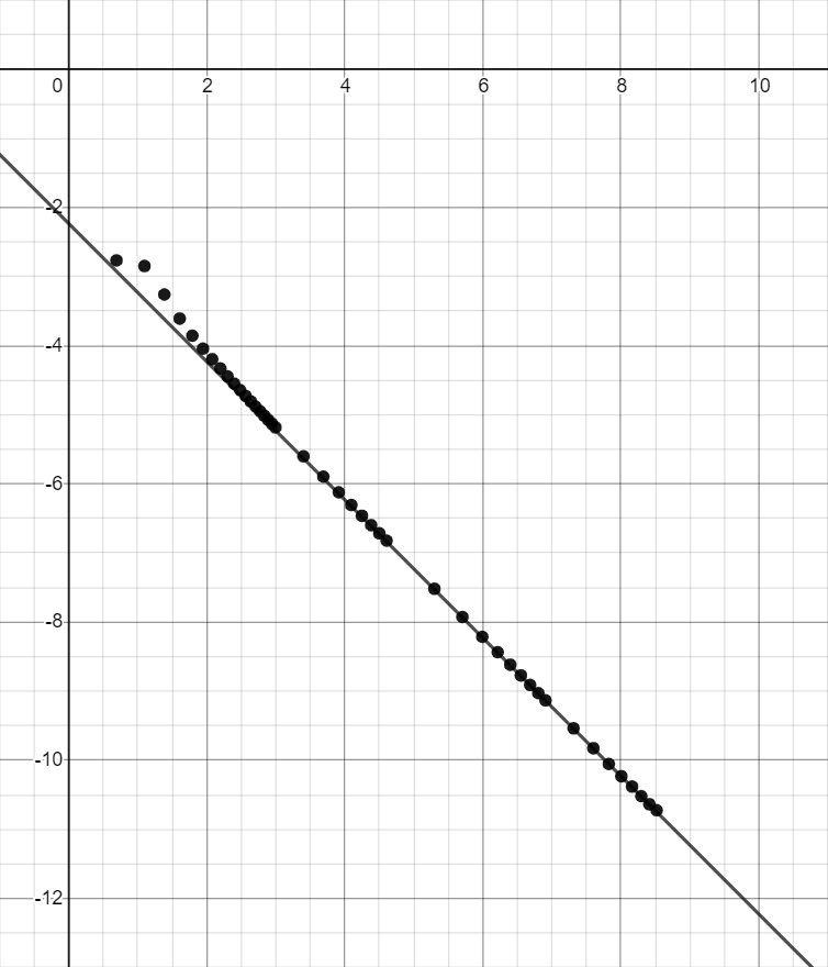
For large , the points appear to approach a line with slope and -intercept . In other words,
Exponentiating and rearranging terms gives
This suggests the following conjecture.
Conjecture 5.1.
There exists a constant such that
5.2 Congruence Conjecture
Theorem 2 of [7] states that if is prime and , then
where is Euler’s totient function. In other words, the Fubini numbers are periodic modulo . Squaring both sides gives the congruence
for prime and . Replacing with suggests the following conjecture, which is supported by the computed values of for .
Conjecture 5.2.
If is prime and , then
Unfortunately, this conjecture does not appear to imply anything about the behavior of the sequence modulo , because of the division by when converting from to .
6 Acknowledgements
Many thanks to Sara Billey for proposing the problem and for helpful discussions, and to the WXML (Washington Experimental Mathematics Lab) for providing the project that led to this paper. Also thanks to Sara Billey and the anonymous referees for their comments and suggestions on this paper.
7 Web Resources
The basic and memory-optimized implementations of the algorithm described in section 3.6 and the values of for can be found at
| https://github.com/tb65536/ParabolicDoubleCosets |
8 Appendix: Values of
|
References
- [1] S. Billey, M. Konvalinka, T. K. Peterson, W. Slofstra, and B. E. Tenner. Parabolic Double Cosets in Coxeter Groups. The Electronic Journal of Combinatorics, 25(1), 2018.
- [2] P. Diaconis and A. Gangolli. Rectangular Arrays with Fixed Margins. Discrete Probability and Algorithms, pages 15-41. The IMA Volumes in Mathematics and its Applications, vol 72, 1995. Springer, New York.
- [3] M. Kobayashi. Two-Sided Structure of Double Cosets in Coxeter Groups, June 2011. Accessed online October 2018.
- [4] L. Moser and M. Wyman. Asymptotic Development of the Stirling Numbers of the First Kind. Journal of the London Mathematical Society, 33(2):131-146, 1958.
- [5] The On-Line Encyclopedia of Integer Sequences, published electronically at https://oeis.org, October 2018.
- [6] T. K. Petersen. A two-sided analogue of the Coxeter complex. The Electronic Journal of Combinatorics, 25(4), 2018.
- [7] B. Poonen. Periodicity of a Combinatorial Sequence. The Fibonacci Quarterly, 26(1), 1988.
- [8] J. Riordan. An Introduction to Combinatorial Analysis. Princeton University Press, 1978.
- [9] H. S. Wilf. generatingfunctionology. Accessed online on August 2020.