Counterfactual Prediction Under Outcome Measurement Error
Abstract.
Across domains such as medicine, employment, and criminal justice, predictive models often target labels that imperfectly reflect the outcomes of interest to experts and policymakers. For example, clinical risk assessments deployed to inform physician decision-making often predict measures of healthcare utilization (e.g., costs, hospitalization) as a proxy for patient medical need. These proxies can be subject to outcome measurement error when they systematically differ from the target outcome they are intended to measure. However, prior modeling efforts to characterize and mitigate outcome measurement error overlook the fact that the decision being informed by a model often serves as a risk-mitigating intervention that impacts the target outcome of interest and its recorded proxy. Thus, in these settings, addressing measurement error requires counterfactual modeling of treatment effects on outcomes. In this work, we study intersectional threats to model reliability introduced by outcome measurement error, treatment effects, and selection bias from historical decision-making policies. We develop an unbiased risk minimization method which, given knowledge of proxy measurement error properties, corrects for the combined effects of these challenges. We also develop a method for estimating treatment-dependent measurement error parameters when these are unknown in advance. We demonstrate the utility of our approach theoretically and via experiments on real-world data from randomized controlled trials conducted in healthcare and employment domains. As importantly, we demonstrate that models correcting for outcome measurement error or treatment effects alone suffer from considerable reliability limitations. Our work underscores the importance of considering intersectional threats to model validity during the design and evaluation of predictive models for decision support.
1. Introduction
Algorithmic risk assessment instruments (RAIs) often target labels that imperfectly reflect the goals of experts and policymakers. For example, clinical risk assessments used to inform physician treatment decisions target future utilization of medical resources (e.g., cost, medical diagnoses) as a proxy for patient medical need (Obermeyer et al., 2019; Mullainathan and Obermeyer, 2021, 2017). Predictive models used to inform personalized learning interventions target student test scores as a proxy for learning outcomes (Hur et al., 2022). Yet, these proxies are subject to outcome measurement error (OME) when they systematically differ from the target outcome of interest to domain experts. Unaddressed, OME can be highly consequential: models targeting poor proxies have been linked to misallocation of medical resources (Obermeyer et al., 2019), unwarranted teacher firings (Turque, 2012), and over-policing of minority communities (Butcher et al., 2022). Given its prevalence and implications, increasing research focus has shifted to understanding and mitigating sources of statistical bias impacting proxy outcomes (De-Arteaga et al., 2021; Fogliato et al., 2020, 2021; Wang et al., 2021; Natarajan et al., 2013; Menon et al., 2015).
However, prior work modeling outcome measurement error makes a critical assumption that the decision informed by the algorithm does not impact downstream outcomes. Yet this assumption is often unreasonable in decision support applications, where decisions constitute interventions that impact the policy-relevant target outcome and its recorded proxy (Coston et al., 2020b). For example, in clinical decision support, medical treatments act as risk-mitigating interventions designed to avert adverse health outcomes. However, in the process of selecting a treatment option, a physician will also influence measured proxies (e.g., medical cost, disease diagnoses) (Obermeyer et al., 2019; Mullainathan and Obermeyer, 2021, 2017). As a result, the measurement error characteristics of proxies can vary across the treatment options informed by an algorithm.
In this work, we develop a counterfactual prediction method that corrects for outcome measurement error, treatment effects, and selection bias in parallel. Our method builds upon unbiased risk minimization techniques developed in the label noise literature (Natarajan et al., 2013; Patrini et al., 2017; Chou et al., 2020; Van Rooyen et al., 2015a). Given knowledge of measurement error parameters, unbiased risk minimization methods recover an estimator for target outcomes by minimizing a surrogate loss over proxy outcomes. However, existing methods are not designed for interventional settings whereby decisions impact outcomes – a limitation that we show severely limits model reliability. Therefore, we develop an unbiased risk minimization technique designed for learning counterfactual models from observational data. We compare our approach against models that correct for OME or treatment effects in isolation by conducting experiments on semi-synthetic data from healthcare and employment domains (Finkelstein et al., 2012; LaLonde, 1986; Smith and Todd, 2005). Results validate the efficacy of our risk minimization approach and underscore the need to carefully vet measurement-related assumptions in consultation with domain experts. Our empirical results also surface systematic model failures introduced by correcting for OME or treatment effects in isolation. To our knowledge, our holistic evaluation is the first to examine how outcome measurement error, treatment effects, and selection bias interact to impact model reliability under controlled conditions.
We provide the following contributions: 1) We derive a problem formulation that models interactions between OME, treatment effects, and selection bias ( 3); 2) We develop a novel approach for learning counterfactual models in the presence of OME ( 4.1). We provide a flexible approach for estimating measurement error rates when these are unknown in advance ( 4.2); 3) We conduct synthetic and semi-synthetic experiments to validate our approach and highlight reliability issues introduced by modeling OME or treatment effects in isolation ( 5).
2. Background and related work
2.1. AI functionality and validity concerns
Prior work has conducted detailed assessments of specific modeling issues (Lakkaraju et al., 2017; De-Arteaga et al., 2021; Kleinberg et al., 2018; Coston et al., 2020b; Kallus and Zhou, 2018; Wang et al., 2021), which have been synthesized into broader critiques of AI validity and functionality (Coston et al., 2022; Raji et al., 2022; Wang et al., 2022). Raji et al. (2022) surface AI functionality harms in which models fail to achieve their purported goal due to systematic design, engineering, deployment, and communication failures. Coston et al. (2022) highlight challenges related to value alignment, reliability, and validity that may draw the justifiability of RAIs into question in some contexts. We build upon this literature by studying intersectional threats to model reliability arising from outcome measurement error (Jacobs and Wallach, 2021; Wang et al., 2021), treatment effects (Coston et al., 2020b; Perdomo et al., 2020), and selection bias (Kallus and Zhou, 2018) in parallel.
A Motivating Example. We illustrate the importance of considering interactions between OME and treatment effects by revisiting a widely known audit of an algorithm used to inform screening decisions for a high-risk medical care program (Obermeyer et al., 2019). This audit surfaced measurement error in a “cost of medical care” outcome targeted as a proxy for patient medical need. Critically, the measurement error analysis performed by Obermeyer et al. (2019) assumes that program enrollment status is independent of downstream cost and medical outcomes. Sample FPR FNR Full population 0.37 0.38 Unenrolled 0.37 0.39 Enrolled 0.64 0.13 Yet our re-analysis shows that the “cost of medical care” proxy has a substantially higher false positive rate and lower false negative rate among program enrollees as compared to the full population (see Appendix A.1). This error rate discrepancy is consistent with enrollees receiving closer medical supervision (and as a result, greater costs), even after accounting for their underlying medical need. In this work, we show that failing to model the interactions between OME and treatment effects can introduce substantial model reliability challenges.
2.2. Outcome measurement error
Modeling outcome measurement error is challenging because it introduces two sources of uncertainty: which error model is reasonable for a given proxy, and which specific error parameters govern the relationship between target and proxy outcomes under the assumed measurement model (Jacobs and Wallach, 2021). Popular error models studied in the machine learning literature include uniform (Angluin and Laird, 1988; Van Rooyen et al., 2015b), class-conditional (Menon et al., 2015; Scott et al., 2013), and instance-dependent (Xia et al., 2020; Chen et al., 2021) structures of outcome misclassification. Work in algorithmic fairness has also studied settings in which measurement error varies across levels of a protected attribute (Wang et al., 2021), and proposed sensitivity analysis frameworks that are model agnostic(Fogliato et al., 2020).
Numerous statistical approaches have been developed for measurement error parameter estimation in the quantitative social sciences literature (Roberts, 1985; Bishop, 1998). Application of these approaches is tightly coupled with domain knowledge of the phenomena under study, as in biostatistics (Hui and Walter, 1980) or psychometrics (Shrout and Lane, 2012). To date, data-driven techniques for error parameter estimation have primarily been applied in the machine learning literature, which rely on key assumptions relating the target outcome of interest and its proxy (Xia et al., 2019; Liu and Tao, 2015; Scott, 2015; Scott et al., 2013; Menon et al., 2015; Northcutt et al., 2021). In this work, we build upon an existing “anchor assumptions” framework that estimates error parameters by linking the proxy and target outcome probabilities at specific instances (Xia et al., 2019). In contrast to prior work, we provide a range of anchoring assumptions, which can be flexibly combined depending on which are reasonable in a specific algorithmic decision support (ADS) domain.
Natarajan et al. (2013) propose a widely-adopted unbiased risk minimization approach for learning under noisy labels given knowledge of measurement error parameters (Patrini et al., 2017; Chou et al., 2020; Van Rooyen et al., 2015a). This method constructs a surrogate loss such that the -risk over proxy outcomes is equivalent to the -risk over target outcomes in expectation. Additionally, Natarajan et al. (2013) show that the minimizer of -risk over proxy outcomes is optimal with respect to target outcomes if is symmetric (e.g., Huber, logistic, and squared losses). In this work, we develop a novel variant of this unbiased risk minimization approach designed for settings with treatment-conditional OME.

2.3. Counterfactual prediction
Recent work has shown that counterfactual modeling is necessary when the decision informed by a predictive model serves as a risk-mitigating intervention (Coston et al., 2020b). Building off of this result, we argue that it is necessary to account for treatment effects on target outcomes of interest and their observed proxy while modeling OME. Our methods build upon conditional average treatment effect (CATE) estimation techniques from the causal inference literature (Shalit et al., 2017; Johansson et al., 2020; Abrevaya et al., 2015). Subject to identification conditions (Pearl, 2009; Rubin, 2005), these approaches predict the difference between the expected outcome under treatment (e.g., high-risk program enrollment) versus control (e.g., no program enrollment) conditional on covariates. One family of outcome regression estimators predicts the CATE by directly estimating the expected outcome under treatment or control conditional on covariates (Hill, 2011; Künzel et al., 2019; Chernozhukov et al., 2017). However, these methods suffer from statistical bias when prior decisions were non-randomized (i.e., due to distribution shift induced by selection bias) (Shimodaira, 2000; Angluin and Laird, 1988). Therefore, we leverage a re-weighting strategy proposed by (Johansson et al., 2020) to correct for this selection bias during risk minimization. Our re-weighting method performs a similar bias correction as inverse probability weighting (IPW) methods (Shimodaira, 2000, 2000; Rosenbaum and Rubin, 1983).
Outcome measurement error has also been studied in causal inference literature. Finkelstein et al. (2021) bound the average treatment effect (ATE) under multiple plausible OME models. Shu and Yi (2019) propose a doubly robust method which accounts for measurement error during ATE estimation, while Díaz and van der Laan (2013) provide a sensitivity analysis framework for examining robustness of ATE estimates to OME. This work is primarily concerned with estimating population statistics rather than predicting outcomes conditional on measured covariates (i.e., the CATE).
3. Preliminaries
Let be a fixed joint distribution over covariates , past decisions111We also use the word treatments to refer to binary decisions. This draws upon historical applications of causal inference to medical settings. , target potential outcomes , and proxy potential outcomes . Under the potential outcomes framework (Rubin, 2005), and are the target and proxy outcomes that would occur under and , respectively (Figure 1). Building upon the class-conditional model studied in observational settings (Natarajan et al., 2013; Menon et al., 2015), we propose a treatment-conditional outcome measurement error model, whereby the class probability of the proxy potential outcome is given by
| (1) |
where , are the proxy false positive and false negative rates under treatment such that . This model imposes the following assumption on the structure of measurement error.
Assumption 1 (Measurement error).
Measurement error rates are fixed across covariates: .
While we make this assumption to foreground study of treatment effects, our methods are also compatible with approaches designed for error rates that vary across covariates (Wang et al., 2021) (see 6.1 for discussion). Given the joint , we would like to estimate , for any target covariates , which is the probability of the target potential outcome under intervention . However, rather than observing directly, we sample from an observational distribution , where is an observed proxy outcome. By consistency, the unobserved target potential outcome and observed proxy potential outcome is determined by the treatment assignment.
Assumption 2 (Consistency).
.
This assumption holds that the target and proxy potential outcomes are observed among instances assigned to treatment (Pearl, 2009; Rubin, 2005, 1974). To identify observational proxy outcomes , we also require the following additional causal assumptions.
Assumption 3 (Ignorability).
. This holds that target and proxy potential outcomes are unconfounded given measured covariates .
Ignorability can be violated in decision support applications when unobservables impact both the treatment and outcome (Kleinberg et al., 2018; Lakkaraju et al., 2017; De-Arteaga et al., 2021). Understanding and addressing limitations introduced by ignorability is a major ongoing research focus (Díaz and van der Laan, 2013; Rambachan et al., 2022; Coston et al., 2020b). We provide follow-up discussion of this assumption in 6.2.
Assumption 4 (Positivity).
. This holds that each instance has some chance of receiving each decision .
Positivity is often reasonable in decision support applications because instances that require support from predictive models are subject to discretionary judgement due to uncertainty. Instances that are certain to receive a given treatment (i.e., or ) would normally be routed via a different administrative procedure. Figure 2 shows a causal diagram representing the data generating process we study in this work.
4. Methodology
We begin by developing an unbiased risk minimization approach which recovers an estimator for given knowledge of error parameters ( 4.1). We then provide a method for estimating and when error parameters are unknown in advance ( 4.2).
4.1. Unbiased risk minimization
In this section, we develop an approach for estimating given observational data drawn from and measurement error parameters , . Let for be a probabilistic decision function targeting and let be a loss function. If we observed target potential outcomes , we could directly apply supervised learning techniques to minimize the expected -risk of over target potential outcomes
| (2) |
and learn an estimator for via standard empirical risk minimization approaches. Given a strongly proper composite loss such that is a monotone transform of (e.g., the logistic and exponential loss), this would enable recovering class probabilities from the optimal prediction via the link function (Agarwal, 2014; Menon et al., 2015). However, directly minimizing (2) is not possible in our setting because we sample observational proxies instead of target potential outcomes. We address this challenge by constructing a re-weighted surrogate risk such that evaluating this risk over observed proxy outcomes is equivalent to in expectation.
In particular, let be a weighting function satisfying and let be a surrogate loss function. We construct a re-weighted surrogate risk
| (3) |
such that in expectation. Theorem 4.1 shows that we can recover a surrogate risk satisfying this property by constructing as in (4) and as in (5). Note that this surrogate risk requires knowledge of , .
Theorem 4.1.
We prove Theorem 4.1 in Appendix A.2. Intuitively, applies a joint bias correction for OME and distribution shift introduced by historical decision-making policies (i.e., selection bias). The unbiased risk minimization framework dating back to Natarajan et al. (2013) corrects for OME by minimizing a surrogate loss on proxies observed over the full population unconditional on treatment. Yet this approach is untenable when decisions impact outcomes () and error rates differ across treatments. One possible extension of unbiased risk minimizers to the treatment-conditional setting involves minimizing over the treatment population
| (6) |
However, in observational settings because the treatment population can differ from the marginal population under historical selection policies when . Therefore, our re-weighting procedure applies a second bias correction that adjusts to resemble .
Learning algorithm. As a result of Theorem 4.1, we can learn a predictor by minimizing the re-weighted surrogate risk over observed samples . First, we estimate the weighting function through a finite sample, which boils down to learning propensity scores (as shown in (4)). Estimating the propensity scores can be done by applying supervised learning algorithms to learn a predictor from to . Then for any treatment , weighting function , and predictor , we can approximate by taking the sample average over the treatment population
| (7) |
for . Therefore, given we can learn a predictor from observational data by minimizing the empirical risk
| (8) |
We refer to solving (8) as re-weighted risk minimization with a surrogate loss (Algorithm 1).
4.2. Error parameter identification and estimation
Because our risk minimization approach requires knowledge of OME parameters, we develop a method for estimating , from observational data. Error parameter estimation is challenging in decision support applications because target outcomes often result from nuanced social and organizational processes. Understanding the measurement error properties of proxies targeted in criminal justice, medicine, and hiring domains remains an ongoing focus of domain-specific research (Fogliato et al., 2021; Akpinar et al., 2021; Mullainathan and Obermeyer, 2021; Obermeyer et al., 2019; Zwaan and Singh, 2015; Chalfin et al., 2016). Therefore, we develop an approach compatible with multiple sources of domain knowledge about proxies, which can be flexibly combined depending on which assumptions are deemed reasonable in a specific context.
Error parameters are identifiable if they can be uniquely computed from observational data. Because our error model (e.q. 1) expresses the proxy class probability as a linear equation with two unknowns, , are identifiable if the target class probability and proxy class probability are known at two distinct points and such that . Following prior literature (Han et al., 2020), we refer to knowledge of as an anchor assumption because it requires knowledge of the unobserved quantity . We now introduce several anchor assumptions that are practical in ADS, before showing that these can be flexibly combined to identify , in Theorem 4.2.
Min anchor. A min anchor assumption holds if there is an instance at no risk of the target potential outcome under intervention : . Because is a strictly monotone increasing transform of , the corresponding value of can be recovered via (Menon et al., 2015). Min anchors are reasonable when there are cases that are confirmed to be at no risk based on domain knowledge of the data generating process. For example, a min anchor may be reasonable in diagnostic testing if a patient is confirmed to be negative for a medical condition based on a high-precision gold standard medical test (Enøe et al., 2000).
Max anchor. A max anchor assumption holds if there is an instance at certain risk of the target outcome under intervention : . The corresponding value of can be recovered via because is a strictly monotone increasing transform of . Max anchors are reasonable when there are confirmed instances of a positive target potential outcome based on domain knowledge of the data generating process. For example, a max anchor may be justified in a medical setting if a subset of patients have confirmed disease diagnoses based on biopsy results (Begg and Greenes, 1983), or if a disease prognosis (and resulting health outcomes) are known from pathology.
Base rate anchor. A base rate anchor assumption holds if the expected value of is known under intervention : . The corresponding value of can be recovered by taking the expectation over the proxy class probability . Base rate anchors are practical because the prevalence of unobservable target outcomes (e.g., medical conditions (Walter and Irwig, 1988), crime (Kruttschnitt et al., 2014; Lohr, 2019), student performance (Schouwenburg, 2004; Di Folco et al., 2022)) is routinely estimated via domain-specific analyses of measurement error. For instance, studies have been conducted to estimate the base rate of undiagnosed heart attacks (i.e., accounting for measurement error in diagnosis proxy outcomes) (Orso et al., 2017). Additionally, the conditional average treatment effect is commonly estimated in randomized controlled trials (RCTs) while assessing treatment effect heterogeneity (Hill, 2011). While the conditional average treatment effect is normally estimated via proxies and , measurement error analysis is a routine component of RCT design and evaluation (Gamerman et al., 2019).
Anchor assumptions can be flexibly combined to identify error parameters based on which set of assumptions are reasonable in a given ADS domain. In particular, Theorem 4.2 shows that combinations of anchor assumptions listed in Table 1 are sufficient for identifying error parameters under our causal assumptions.
| Know | Min | Base rate | Max | Know | |
|---|---|---|---|---|---|
| Know | ✕ | ✕ | ✓ | ✓ | ✓ |
| Min | ✕ | ✕ | ✓ | ✓ | ✓ |
| Base rate | ✓ | ✓ | ✕ | ✓ | ✓ |
| Max | ✓ | ✓ | ✓ | ✕ | ✕ |
| Know | ✓ | ✓ | ✓ | ✕ | ✕ |
Theorem 4.2.
We prove Theorem 4.2 in Appendix A.2. In practice, we estimate the error rates on finite samples , which gives an approximation . Therefore, we propose a conditional class probability estimation (CCPE) method for parameter estimation which estimates , by fitting on observational data then applying the relevant pair of anchor assumptions to estimate error rates. Algorithm 2 provides pseudocode for this approach with min and max anchors, which can easily be extended to other pairs of identifying assumptions shown in Table 1. The combination of min and max anchors is known as weak separability (Menon et al., 2015) or mutual irreducibility (Scott et al., 2013; Scott, 2015) in the observational label noise literature. Prior results in the observational setting show that unconditional class probability estimation (i.e., fitting )) yields a consistent estimator for observational error rates under weak seperability (Scott et al., 2013; Reeve et al., 2019). Statistical consistency results extend to the treatment-conditional setting under positivity (4) because . However, asymptotic convergence rates may be slower under strong selection bias if is near 0.
5. Experiments
Experimental evaluation under treatment-conditional OME is challenging due to compounding sources of uncertainty. We do not observe counterfactual outcomes in historical data, making it challenging to estimate the quality of new models via observational data. Further, because the target outcome is not observed directly, we rely on measurement assumptions when studying proxy outcomes in naturalistic data. We address this challenge by conducting a controlled evaluation with synthetic data where ground truth potential outcomes are fully observed. To better reflect the ecological settings of real-world deployments, we also conduct a semi-synthetic evaluation with real data collected through randomized controlled trials (RCTs) in healthcare and employment domains. Our evaluation (1) validates our proposed risk minimization approach, (2) underscores the need to carefully consider measurement assumptions during error rate estimation, and (3) shows that correcting for OME or treatment effects in isolation is insufficient.222Code for all experiments can be found at: https://github.com/lguerdan/CP_OME.
5.1. Models
We compare several modeling approaches in our evaluation to examine how existing modeling practices are impacted by treatment-conditional outcome measurement error:
-
•
Unconditional proxy (UP). Predict the observed outcome unconditional on treatment: . This model does not adjust for OME or treatment effects., and reflects model performance in a scenario in which practitioners overlook all challenges examined in this work. 333This baseline is also called an observational risk assessment in experiments reported by Coston et al. (2020b).
-
•
Unconditional target (UT). Predict the target outcome unconditional on treatment: . Here, we determine by applying consistency: . This method reflects a setting in which no OME is present but modeling does not account for treatment effects (Wang et al., 2021; Natarajan et al., 2013; Menon et al., 2015; Obermeyer et al., 2019).
-
•
Conditional proxy (CP). Predict the proxy outcome conditional on treatment: . This is a counterfactual model that estimates a conditional expectation without correcting for OME (Coston et al., 2020b; Shalit et al., 2017; Künzel et al., 2019).444This model is known by different names in the causal inference literature, including the backdoor adjustment (G-computation) formula (Pearl, 2009; Robins, 1986), T-learner (Künzel et al., 2019), and plug-in estimator (Kennedy, 2022).
-
•
Re-weighted surrogate loss (RW-SL). Our proposed risk minimization approach, as defined in equation (8). This method corrects for both OME and treatment effects in parallel. Additionally, this method corrects for distribution shift due to selection bias in the prior decision-making policy via re-weighting.
-
•
Target Potential Outcome (TPO). Directly predict the target potential outcome: . This model is an oracle that provides an upper-bound on model performance under no OME or treatment effects.
We also perform an ablation of our proposed RW-SL method by including a model that applies a surrogate loss correction over the treatment population without re-weighting (SL).


| (0.0, 0.4) | (0.1, 0.3) | (0.2, 0.2) | (0.3, 0.1) | (0.4, 0.0) | |
| UP | 54.18 (0.09) | 53.00 (0.39) | 54.89 (1.09) | 55.81 (0.74) | 46.76 (0.33) |
| UT | 61.57 (0.63) | 60.95 (0.50) | 60.49 (0.41) | 61.00 (0.49) | 60.54 (0.70) |
| CP | 51.36 (1.83) | 68.24 (2.61) | 75.05 (0.92) | 67.77 (1.33) | 61.88 (0.28) |
| SL | 72.38 (1.65) | 65.45 (0.66) | 67.43 (1.64) | 68.01 (0.99) | 65.92 (1.34) |
| RW-SL | 69.08 (1.55) | 65.96 (1.18) | 66.57 (1.32) | 68.39 (1.33) | 64.56 (0.52) |
| SL | 67.09 (1.24) | 67.58 (1.19) | 67.75 (1.08) | 69.11 (1.17) | 68.59 (1.41) |
| RW-SL | 73.68 (1.49) | 73.39 (1.60) | 72.52 (1.66) | 74.34 (1.15) | 75.01 (1.24) |
| TPO | 77.08 (0.11) | 77.09 (0.20) | 76.98 (0.08) | 76.84 (0.18) | 76.90 (0.16) |
5.2. Experiments on synthetic data
We begin by experimentally manipulating treatment effects and measurement error via a synthetic evaluation. Because this provides full control over the data generating process, we can evaluate methods against target potential outcomes. This evaluation would not possible with real-world data because counterfactual target outcomes are unobserved. Our experiment design is consistent with prior synthetic evaluations of counterfactual risk assessments (Coston et al., 2020b) and causal inference methods (Shi et al., 2019; Nie et al., 2021). In our evaluation, we sample outcomes via the following data generating process:
-
(1)
-
(2)
-
(3)
-
(4)
As shown in Figure 4, we draw and sample target potential outcomes from sinusoidal class probability functions (see Appendix A.4 for details). Note that our choice of , satisfies min and max anchor assumptions. Because and differ, models that do not condition on treatment (i.e., UP, UT) will learn an average of the two class probability functions. Under our choice of , fewer samples are drawn from in the region where is small (near ), and fewer samples are drawn from in the region where is small (near ). This introduces selection bias when sampling from .
5.2.1. Setup details
We train each model in 5.1 to predict risk under no intervention () and vary . We keep fixed at across settings. When estimating OME parameters, we run CCPE with sample splitting and cross-fitting (Algorithm 4) with min and max anchor assumptions for identification. These assumptions hold precisely under this controlled evaluation (Figure 4). We run all methods with sample splitting and cross-fitting (Algorithm 3) and report performance on .
5.2.2. Results
Figure 4 shows the performance of each model as a function of sample size. TPO provides an upper bound on performance because it learns directly from target potential outcomes. RW-SL with oracle parameters outperforms all other methods trained on observational data across across the full range of sample sizes. Thus, while Thm. 4.1 shows that RW-SL recovers an unbiased risk estimator in expectation, this method also demonstrates favorable finite-sample performance characteristics in practice. This finding is inline with prior experimental evaluations of unbiased risk estimators reported in the standard supervised learning setting (Natarajan et al., 2013; Wang et al., 2021), and is further supported by reliable performance characteristics we observe in small sample regimes (see Appendix A.4).
In contrast, both models that do not condition on treatment (UP and UT), and the conditional regression trained on proxy outcomes (CP), reach a performance plateau by 50k samples and do not benefit from additional data. This indicates that (1) learning a counterfactual model and (2) correcting for measurement error is necessary to learn in this evaluation. We likely observe a sharper plateau in UP and UT above 20k samples because these approaches fit a weighted average of and (where differs from considerably). We observe that RW-SL and SL performance deteriorates with learned parameters across all sample size settings due to misspecification in learned parameter estimates and weights.
Table 2 shows a breakdown across error rates at samples. RW-SL outperforms SL when oracle parameters are known. However, RW-SL and SL perform comparably when weights and parameters are learned. This may be because RW-SL relies on estimates in addition to , which could introduce instability given misspecification in . CP performs notably well under high error parameter symmetry (i.e., ). This is consistent with prior results from the class-conditional label noise literature (Natarajan et al., 2013; Menon et al., 2015), which show that the optimal classifier threshold for misclassification risk does not change under symmetric label noise. CP performs worse under high error asymmetry. We do not observe a similar performance improvement in UP and UT in the symmetric error setting because these baselines learn a weighted combination of and , which differs from the target function at all classification thresholds.
5.3. Semi-synthetic experiments on healthcare and employment data
In addition to our synthetic evaluation, we conduct experiments using real-world data collected as part of randomized controlled trials (RCTs) in healthcare and employment domains. While this evaluation affords less control over the data generating process, it provides a more realistic sample of data likely to be encountered in real-world model deployments. Evaluation via data from randomized or partially randomized experimental studies is useful for validating counterfactual prediction approaches because random assignment ensures that causal assumptions are satisfied (Shalit et al., 2017; Johansson et al., 2020; Coston et al., 2020a).
5.3.1. Randomized Controlled Trial (RCT) Datasets
In 2008, the U.S. state of Oregon expanded access to its Medicare program via a lottery system (Finkelstein et al., 2012). This lottery provided an opportunity to study the effects of Medicare enrollment on healthcare utilization and medical outcomes via an experimental design, commonly referred to as the Oregon Health Insurance Experiment (OHIE). Lottery enrollees completed a pre-randomization survey recording demographic factors and baseline health status and were given a one-year follow-up assessment of health status and medical care utilization. We refer the reader to Finkelstein et al. (2012) for details. We use the OHIE dataset to construct an evaluation task that parallels the label choice bias analysis of Obermeyer et al. (2019). We use this dataset rather than synthetic data released by Obermeyer et al. (2019) because (1) treatment was randomly assigned, ruling out positivity and ignorability violations possible in observational data, and (2) OHIE data contains covariates necessary for predictive modeling. We predict diagnosis with an active chronic medical condition over the one-year follow-up period given covariates, including health history, prior emergency room visits, and public services use. We predict chronic health conditions because findings from Obermeyer et al. (2019) indicate that this outcome variable is a reasonable choice of proxy for patient medical need. We adopt the randomized lottery draw as the treatment. 555The OHIE experiment had imperfect compliance ( 30 percent of selected individuals successfully enrolled (Finkelstein et al., 2012)). Therefore, we predict diagnosis with a new chronic health condition given the opportunity to enroll in Medicare. This evaluation is consistent with many high-stakes decision-support settings granting opportunities to individuals, which they have a choice to pursue if desired.
We conduct a second real-world evaluation using the JOBS dataset, which investigates the effect of job retraining on employment status (Shalit et al., 2017). This dataset includes an experimental sample collected by LaLonde (1986) via the National Supported Work (NSW) program (297 treated, 425 control) consisting primarily of low-income individuals seeking job retraining. Smith and Todd (2005) combine this sample with a “PSID” comparison group (2,490 control) collected from the general population, which resulted in a final sample with 297 treated and 2,915 control. This dataset includes covariates including age, education, prior earnings, and interaction terms. 482 (15%) of subjects were unemployed at the end of the study. Following Johansson et al. (2020), we construct an evaluation task predicting unemployment under enrollment () and no enrollment () in a job retraining program conditional on covariates.
5.3.2. Synthetic OME and selection bias
We experimentally manipulate OME to examine how outcome regressions perform under treatment-conditional error of known magnitude. We adopt diagnosis with a new chronic condition and future unemployment as a target outcome for OHIE and JOBS, respectively. We observe proxy outcomes by flipping target outcomes with probability (, ). We keep (, ) fixed at . This procedure of generating proxy outcomes by flipping available labels is a common approach for vetting the feasibility of new methodologies designed to address OME (Wang et al., 2021; Menon et al., 2015; Natarajan et al., 2013). This approach offers precise control over the magnitude of OME but suffers from less ecological validity than studying multiple naturalistic proxies (Obermeyer et al., 2019). We opt for this semi-synthetic evaluation because (1) the precise measurement relationship between naturally occurring proxies may not be fully known, (2) the measurement relationship between naturally occurring proxies cannot be manipulated experimentally, and (3) there are few RCT datasets (i.e., required to guarantee causal assumptions) that contain multiple proxies of the same target outcome.
Models used for decision support are typically trained using data gathered under a historical decision-making policy. When prior decisions were made non-randomly, this introduces selection bias () and causes distribution shift between the population that received treatment in training data, and the full population encountered at deployment time. Therefore, we emulate selection bias in the training dataset, and evaluate models over a held-out test set of randomized data. We insert selection bias in OHIE data by removing individuals from the treatment (lottery winning) arm with household income above the federal poverty line (10% of the treatment sample). This resembles an observational setting in which low-income individuals are more likely to receive an opportunity to enroll in a health insurance program (e.g., Medicaid, which determines eligibility based on household income in relation to the federal poverty line). We restrict our analysis to single-person households, yielding total samples ( treatment, control).
We model selection bias in JOBS data by including samples from the observational and experimental cohorts in the training data. Because the PSID comparison group consists of individuals with higher income and education than the NSW group, there is considerable distribution shift across the NSW and PSID cohorts (LaLonde, 1986; Smith and Todd, 2005; Johansson et al., 2020). Therefore, a model predicting unemployment over the control population (consisting of NSW and PSID samples) may suffer from bias when evaluated against test data that only includes samples from the NSW experimental arm. Thus we split data from the NSW experimental cohort 50-50 across training and test dataset, and only include PSID data in the training dataset.
5.3.3. Experimental setup
We include a Conditional Target (CT) model in place of a TPO model because counterfactual outcomes are not available in experimental data. CT provides a reasonable upper-bound on performance because identifiability conditions are satisfied in an experimental setting (Pearl, 2009). However, it is not possible to report accuracy over potential outcomes because counterfactual outcomes are unobserved. Therefore, we report error in ATE estimates , for
where corresponds to the ground-truth treatment effect reported by prior work (Johansson et al., 2020; Denteh and Liebert, 2022) and is a learned model discussed in 5.1. One subtlety of this comparison is that our outcome regressions target the conditional average treatment effect, while reflects the ATE across the full population. Following prior evaluations (Johansson et al., 2020), we compare all methods against the ATE because the ground-truth CATE is not available for JOBS or OHIE data. 666 While our insertion of synthetic selection bias (§5.3.2) introduces distribution shift such that differs from , it does not alter ground-truth because the conditional outcome distribution remains unchanged. This setup recreates the unconfounded observational setting in which causal identification assumptions are satisfied (Rubin, 1974). We report results over a test fold of randomized data that does not contain flipped outcomes or selection bias. Appendix A.4 contains additional setup details.
5.3.4. Results
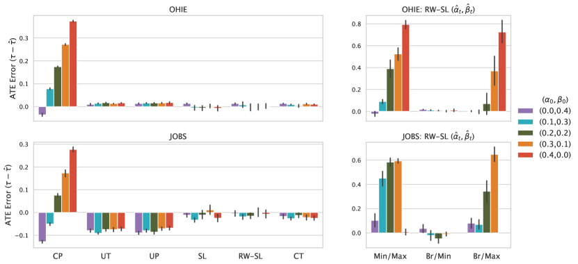
Figure 5 shows bias in ATE estimates over 10 runs on JOBS and OHIE data. The left panel compares CP, UT, UP, and the oracle CT model against RW-SL/SL with oracle parameters , . We show performance of RW-SL with learned parameters , on the right panel. The left panel shows that CP is highly sensitive to measurement error. This is because measurement error introduces bias in estimates of the conditional expectations, which propagates to treatment effect estimates. Because UT and UP do not condition on treatment, they estimate an average of the outcome functions and , and generate predictions near 0. Therefore, while UT and UP perform well on OHIE data due to a small ground-truth ATE (), they perform poorly on JOBS (). SL and RW-SL with oracle parameters , perform comparably to the CT model with oracle access to target outcomes across all measurement error settings.
While we observe that re-weighting improves performance in our synthetic evaluation (given oracle parameters), we do not observe a similar advantage of RW-SL over SL in this experiment. Our results parallel other empirical evaluations of re-weighting for counterfactual modeling tasks on real-world data (e.g., see 3.4.2 in (Coston et al., 2020b)). One potential explanation for this finding is that our predictive model class (multi-layer MLPs) is large enough to learn the target regressions and for OHIE and JOBS data, even after our insertion of synthetic selection bias. As a result, re-weighting may not be required to learn a reasonable estimate of and given available data. This interpretation is supported by strong performance of the oracle CT model.
As shown on the right panel of Figure 5, RW-SL performance is highly sensitive to the choice of anchor assumption used to estimate parameters (, ), (, ) as indicated by increased bias in and greater variability over runs. In particular, RW-SL performs poorly when Min/Max and Br/Max pairs of anchor assumptions are used to estimate error rates because the max anchor assumption is violated on OHIE and JOBS data. We shed further light on this finding by fitting the CT model to estimate , on OHIE data, then computing inferences over a validation fold . This analysis reveals that
which suggests that the min anchor assumption that is reasonable for , while the max anchor assumption that is violated for both . Therefore, because the min anchor assumption is satisfied for these choices of target outcome, and the ground-truth base rate is known in this experimental setting, RW-SL demonstrates strong performance given the Br/Min combination of anchor assumptions. In contrast, because the max anchor is violated, estimating by taking the supremium of introduces bias in , which results in poor performance of RW-SL with Min/Max and Br/Max anchors. Applying this same procedure to the unemployment outcome targeted in JOBS data also reveals a violation of the max anchor assumption. These results underscore the importance of selecting anchor assumptions in close consultation with domain experts because it is not possible to verify anchor assumptions by learning when the target outcome of interest is unobserved.
6. Discussion
In this work, we show the importance of carefully addressing intersectional threats to model reliability during the development and evaluation of predictive models for decision support. Our theoretical and empirical results validate the efficacy of our unbiased risk minimization approach. When OME parameters are known, our method performs comparably to a model with oracle access to target potential outcomes. However, our results underscore the importance of vetting anchoring assumptions used for error parameter estimation before using error rate estimates for risk minimization. Critically, our experimental results also demonstrate that correcting for a single threat to model reliability in isolation is insufficient to address model validity concerns (Raji et al., 2022), and risks promoting false confidence in corrected models. Below, we expand upon key considerations surfaced by our work.
6.1. Decision points and complexities in measurement error modeling
Our work speaks to key complexities faced by domain experts, model developers, and other stakeholders while examining proxies in ADS. One decision surfaced by our work entails which measurement error model best describes the relationship between the unobserved outcome of policy interest and its recorded proxy. We open this work by highlighting a measurement model decision made by Obermeyer et al. (2019) during their audit of a clinical risk assessment: that error rates are fixed across treatments. Our work suggests that failing to account for treatment-conditional error in OME models may exacerbate reliability concerns. However, at the same time, the error model we adopt in this work intentionally abstracts over other factors known to impact proxies in decision support tasks, including error rates that vary across covariates. Although this simplifying assumption can be unreasonable in some settings (Fogliato et al., 2021; Akpinar et al., 2021), including the one studied by Obermeyer et al. (2019), it is helpful in foregrounding previously-overlooked challenges involving treatment effects and selection bias. In practice, model developers correcting for measurement error may wish to combine our methods with existing unbiased risk minimization approaches designed for group-dependent error where appropriate (Wang et al., 2021). Further, analyses of measurement error should not overlook more fundamental conceptual differences between target outcomes and proxies readily available for modeling (e.g., when long-term child welfare related outcomes targeted by a risk assessment differ from immediate threats to child safety weighted by social workers (Kawakami et al., 2022, 2022)). This underscores the need to carefully weigh the validity of proxies in consultation with multiple stakeholders (e.g., domain experts, data scientists, and decision-makers) while deciding whether OME correction is warranted.
A second decision point highlighted in this work entails the specific measurement error parameters that govern the relationship between target and proxy outcomes. In particular, our work underscores the need for a tighter coupling between domain expertise and data-driven approaches for error parameter estimation. Current techniques designed to address OME in the machine learning literature – which typically examine settings with “label noise” – rely heavily upon data-driven approaches without close consideration of whether the underlying measurement assumptions hold (Wang et al., 2021; Northcutt et al., 2021; Menon et al., 2015; Xia et al., 2019). While application of these assumptions may be practical for methodological evaluations and theoretical analysis (Scott et al., 2013; Scott, 2015; Reeve et al., 2019), these assumptions should be carefully vetted when applying OME correction to real-world proxies. This is supported by our findings in Figure 5, which show that RW-SL performs poorly when the anchor assumptions used for error parameter estimation are violated. Our flexible set of anchor assumptions provides a step towards a tighter coupling between domain expertise and data-driven approaches in measurement parameter estimation.
6.2. Challenges of linking causal and statistical estimands
Our counterfactual modeling approach requires several causal identifiability assumptions (Pearl, 2009), which may not be satisfied in all decision support contexts. Of our assumptions, the most stringent is likely ignorability, which requires that no unobserved confounders influenced past decisions and outcomes. While recent modeling developments may ease ignorability-related concerns in some cases (Coston et al., 2020b; Rambachan et al., 2022), model developers should carefully evaluate whether confounders are likely to impact a model in a given deployment context. At the same time, our results show that formulating algorithmic decision support as a “pure prediction problem” that optimizes predictive performance without estimating causal effects (Kleinberg et al., 2015) imposes equally serious limitations. If the policy-relevant target outcome of interest is risk conditional on intervention (as is often the case in decision support applications), an observational model will generate invalid predictions for cases that historically responded most to treatment (Coston et al., 2020b). Our results, which empirically demonstrate poor performance of observational PU and TU models that overlook treatment-effects, corroborate prior findings indicating that counterfactual modeling is required to ensure the reliability of RAIs in decision support settings (Coston et al., 2020b). Taken together, our work suggests that domain experts and model developers should exercise considerable caution while mapping the causal estimand of policy interest to the statistical estimand targeted by a predictive model (Lundberg et al., 2021).
Acknowledgements.
We thank the anonymous reviewers and attendees of the NeurIPS 2022 Workshop on Causality for Real-world Impact for their helpful feedback. This work was supported by an award from the UL Research Institutes through the Center for Advancing Safety of Machine Intelligence (CASMI) at Northwestern University, the Carnegie Mellon University Block Center for Technology and Society (Award No. 53680.1.5007718), and the National Science Foundation Graduate Research Fellowship Program (Award No. DGE-1745016). ZSW is supported in part by an NSF FAI Award (No. 1939606), a Google Faculty Research Award, a J.P. Morgan Faculty Award, a Facebook Research Award, an Okawa Foundation Research Grant, and a Mozilla Research Grant.References
- (1)
- Abrevaya et al. (2015) Jason Abrevaya, Yu-Chin Hsu, and Robert P Lieli. 2015. Estimating conditional average treatment effects. Journal of Business & Economic Statistics 33, 4 (2015), 485–505.
- Agarwal (2014) Shivani Agarwal. 2014. Surrogate regret bounds for bipartite ranking via strongly proper losses. The Journal of Machine Learning Research 15, 1 (2014), 1653–1674.
- Akpinar et al. (2021) Nil-Jana Akpinar, Maria De-Arteaga, and Alexandra Chouldechova. 2021. The effect of differential victim crime reporting on predictive policing systems. In Proceedings of the 2021 ACM conference on fairness, accountability, and transparency. 838–849.
- Angluin and Laird (1988) Dana Angluin and Philip Laird. 1988. Learning from noisy examples. Machine Learning 2, 4 (1988), 343–370.
- Begg and Greenes (1983) Colin B Begg and Robert A Greenes. 1983. Assessment of diagnostic tests when disease verification is subject to selection bias. Biometrics (1983), 207–215.
- Bishop (1998) Christopher M Bishop. 1998. Latent Variable Models. Learning in graphical models 371 (1998).
- Butcher et al. (2022) Bradley Butcher, Chris Robinson, Miri Zilka, Riccardo Fogliato, Carolyn Ashurst, and Adrian Weller. 2022. Racial Disparities in the Enforcement of Marijuana Violations in the US. In Proceedings of the 2022 AAAI/ACM Conference on AI, Ethics, and Society. 130–143.
- Chalfin et al. (2016) Aaron Chalfin, Oren Danieli, Andrew Hillis, Zubin Jelveh, Michael Luca, Jens Ludwig, and Sendhil Mullainathan. 2016. Productivity and selection of human capital with machine learning. American Economic Review 106, 5 (2016), 124–127.
- Chen et al. (2021) Pengfei Chen, Junjie Ye, Guangyong Chen, Jingwei Zhao, and Pheng-Ann Heng. 2021. Beyond class-conditional assumption: A primary attempt to combat instance-dependent label noise. In Proceedings of the AAAI Conference on Artificial Intelligence, Vol. 35. 11442–11450.
- Chernozhukov et al. (2017) Victor Chernozhukov, Denis Chetverikov, Mert Demirer, Esther Duflo, Christian Hansen, and Whitney Newey. 2017. Double/debiased/neyman machine learning of treatment effects. American Economic Review 107, 5 (2017), 261–265.
- Chou et al. (2020) Yu-Ting Chou, Gang Niu, Hsuan-Tien Lin, and Masashi Sugiyama. 2020. Unbiased risk estimators can mislead: A case study of learning with complementary labels. In International Conference on Machine Learning. PMLR, 1929–1938.
- Coston et al. (2020a) Amanda Coston, Edward Kennedy, and Alexandra Chouldechova. 2020a. Counterfactual predictions under runtime confounding. Advances in Neural Information Processing Systems 33 (2020), 4150–4162.
- Coston et al. (2020b) Amanda Coston, Alan Mishler, Edward H Kennedy, and Alexandra Chouldechova. 2020b. Counterfactual risk assessments, evaluation, and fairness. In Proceedings of the 2020 conference on fairness, accountability, and transparency. 582–593.
- Coston et al. (2022) Amanda Lee Coston, Anna Kawakami, Haiyi Zhu, Ken Holstein, and Hoda Heidari. 2022. A Validity Perspective on Evaluating the Justified Use of Data-driven Decision-making Algorithms. First IEEE Conference on Secure and Trustworthy Machine Learning (2022).
- De-Arteaga et al. (2021) Maria De-Arteaga, Artur Dubrawski, and Alexandra Chouldechova. 2021. Leveraging expert consistency to improve algorithmic decision support. arXiv preprint arXiv:2101.09648 (2021).
- Denteh and Liebert (2022) Augustine Denteh and Helge Liebert. 2022. Who Increases Emergency Department Use? New Insights from the Oregon Health Insurance Experiment. arXiv preprint arXiv:2201.07072 (2022).
- Di Folco et al. (2022) Cécile Di Folco, Ava Guez, Hugo Peyre, and Franck Ramus. 2022. Epidemiology of reading disability: A comparison of DSM-5 and ICD-11 criteria. Scientific Studies of Reading 26, 4 (2022), 337–355.
- Díaz and van der Laan (2013) Iván Díaz and Mark J van der Laan. 2013. Sensitivity analysis for causal inference under unmeasured confounding and measurement error problems. The international journal of biostatistics 9, 2 (2013), 149–160.
- Enøe et al. (2000) Claes Enøe, Marios P Georgiadis, and Wesley O Johnson. 2000. Estimation of sensitivity and specificity of diagnostic tests and disease prevalence when the true disease state is unknown. Preventive veterinary medicine 45, 1-2 (2000), 61–81.
- Falagas et al. (2007) ME Falagas, KZ Vardakas, and PI Vergidis. 2007. Under-diagnosis of common chronic diseases: prevalence and impact on human health. International journal of clinical practice 61, 9 (2007), 1569–1579.
- Finkelstein et al. (2012) Amy Finkelstein, Sarah Taubman, Bill Wright, Mira Bernstein, Jonathan Gruber, Joseph P Newhouse, Heidi Allen, Katherine Baicker, and Oregon Health Study Group. 2012. The Oregon health insurance experiment: evidence from the first year. The Quarterly journal of economics 127, 3 (2012), 1057–1106.
- Finkelstein et al. (2021) Noam Finkelstein, Roy Adams, Suchi Saria, and Ilya Shpitser. 2021. Partial identifiability in discrete data with measurement error. In Uncertainty in Artificial Intelligence. PMLR, 1798–1808.
- Fogliato et al. (2020) Riccardo Fogliato, Alexandra Chouldechova, and Max G’Sell. 2020. Fairness evaluation in presence of biased noisy labels. In International Conference on Artificial Intelligence and Statistics. PMLR, 2325–2336.
- Fogliato et al. (2021) Riccardo Fogliato, Alice Xiang, Zachary Lipton, Daniel Nagin, and Alexandra Chouldechova. 2021. On the Validity of Arrest as a Proxy for Offense: Race and the Likelihood of Arrest for Violent Crimes. In Proceedings of the 2021 AAAI/ACM Conference on AI, Ethics, and Society. 100–111.
- Gamerman et al. (2019) Victoria Gamerman, Tianxi Cai, and Amelie Elsäßer. 2019. Pragmatic randomized clinical trials: best practices and statistical guidance. Health Services and Outcomes Research Methodology 19 (2019), 23–35.
- Han et al. (2020) Bo Han, Quanming Yao, Tongliang Liu, Gang Niu, Ivor W Tsang, James T Kwok, and Masashi Sugiyama. 2020. A survey of label-noise representation learning: Past, present and future. arXiv preprint arXiv:2011.04406 (2020).
- Hill (2011) Jennifer L Hill. 2011. Bayesian nonparametric modeling for causal inference. Journal of Computational and Graphical Statistics 20, 1 (2011), 217–240.
- Hui and Walter (1980) Sui L Hui and Steven D Walter. 1980. Estimating the error rates of diagnostic tests. Biometrics (1980), 167–171.
- Hur et al. (2022) Paul Hur, HaeJin Lee, Suma Bhat, and Nigel Bosch. 2022. Using Machine Learning Explainability Methods to Personalize Interventions for Students. International Educational Data Mining Society (2022).
- Jacobs and Wallach (2021) Abigail Z Jacobs and Hanna Wallach. 2021. Measurement and fairness. In Proceedings of the 2021 ACM conference on fairness, accountability, and transparency. 375–385.
- Johansson et al. (2020) Fredrik D Johansson, Uri Shalit, Nathan Kallus, and David Sontag. 2020. Generalization bounds and representation learning for estimation of potential outcomes and causal effects. arXiv preprint arXiv:2001.07426 (2020).
- Kallus and Zhou (2018) Nathan Kallus and Angela Zhou. 2018. Residual unfairness in fair machine learning from prejudiced data. In International Conference on Machine Learning. PMLR, 2439–2448.
- Kawakami et al. (2022) Anna Kawakami, Venkatesh Sivaraman, Hao-Fei Cheng, Logan Stapleton, Yanghuidi Cheng, Diana Qing, Adam Perer, Zhiwei Steven Wu, Haiyi Zhu, and Kenneth Holstein. 2022. Improving Human-AI Partnerships in Child Welfare: Understanding Worker Practices, Challenges, and Desires for Algorithmic Decision Support. In CHI Conference on Human Factors in Computing Systems. 1–18.
- Kennedy (2022) Edward H Kennedy. 2022. Semiparametric doubly robust targeted double machine learning: a review. arXiv preprint arXiv:2203.06469 (2022).
- Kleinberg et al. (2018) Jon Kleinberg, Himabindu Lakkaraju, Jure Leskovec, Jens Ludwig, and Sendhil Mullainathan. 2018. Human decisions and machine predictions. The quarterly journal of economics 133, 1 (2018), 237–293.
- Kleinberg et al. (2015) Jon Kleinberg, Jens Ludwig, Sendhil Mullainathan, and Ziad Obermeyer. 2015. Prediction policy problems. American Economic Review 105, 5 (2015), 491–495.
- Kruttschnitt et al. (2014) Candace Kruttschnitt, William D Kalsbeek, Carol C House, et al. 2014. Estimating the incidence of rape and sexual assault. (2014).
- Künzel et al. (2019) Sören R Künzel, Jasjeet S Sekhon, Peter J Bickel, and Bin Yu. 2019. Metalearners for estimating heterogeneous treatment effects using machine learning. Proceedings of the national academy of sciences 116, 10 (2019), 4156–4165.
- Lakkaraju et al. (2017) Himabindu Lakkaraju, Jon Kleinberg, Jure Leskovec, Jens Ludwig, and Sendhil Mullainathan. 2017. The selective labels problem: Evaluating algorithmic predictions in the presence of unobservables. In Proceedings of the 23rd ACM SIGKDD International Conference on Knowledge Discovery and Data Mining. 275–284.
- LaLonde (1986) Robert J LaLonde. 1986. Evaluating the econometric evaluations of training programs with experimental data. The American economic review (1986), 604–620.
- Liu and Tao (2015) Tongliang Liu and Dacheng Tao. 2015. Classification with noisy labels by importance reweighting. IEEE Transactions on pattern analysis and machine intelligence 38, 3 (2015), 447–461.
- Lohr (2019) Sharon Lohr. 2019. Measuring crime: Behind the statistics. Chapman and Hall/CRC.
- Lundberg et al. (2021) Ian Lundberg, Rebecca Johnson, and Brandon M Stewart. 2021. What is your estimand? Defining the target quantity connects statistical evidence to theory. American Sociological Review 86, 3 (2021), 532–565.
- Menon et al. (2015) Aditya Menon, Brendan Van Rooyen, Cheng Soon Ong, and Bob Williamson. 2015. Learning from corrupted binary labels via class-probability estimation. In International conference on machine learning. PMLR, 125–134.
- Mullainathan and Obermeyer (2017) Sendhil Mullainathan and Ziad Obermeyer. 2017. Does machine learning automate moral hazard and error? American Economic Review 107, 5 (2017), 476–480.
- Mullainathan and Obermeyer (2021) Sendhil Mullainathan and Ziad Obermeyer. 2021. On the inequity of predicting a while hoping for B. In AEA Papers and Proceedings, Vol. 111. 37–42.
- Natarajan et al. (2013) Nagarajan Natarajan, Inderjit S Dhillon, Pradeep K Ravikumar, and Ambuj Tewari. 2013. Learning with noisy labels. Advances in neural information processing systems 26 (2013).
- Nie et al. (2021) Lizhen Nie, Mao Ye, Qiang Liu, and Dan Nicolae. 2021. Vcnet and functional targeted regularization for learning causal effects of continuous treatments. arXiv preprint arXiv:2103.07861 (2021).
- Northcutt et al. (2021) Curtis Northcutt, Lu Jiang, and Isaac Chuang. 2021. Confident learning: Estimating uncertainty in dataset labels. Journal of Artificial Intelligence Research 70 (2021), 1373–1411.
- Obermeyer et al. (2019) Ziad Obermeyer, Brian Powers, Christine Vogeli, and Sendhil Mullainathan. 2019. Dissecting racial bias in an algorithm used to manage the health of populations. Science 366, 6464 (2019), 447–453.
- Orso et al. (2017) Francesco Orso, Gianna Fabbri, and Aldo Pietro Maggioni. 2017. Epidemiology of heart failure. Heart Failure (2017), 15–33.
- Patrini et al. (2017) Giorgio Patrini, Alessandro Rozza, Aditya Krishna Menon, Richard Nock, and Lizhen Qu. 2017. Making deep neural networks robust to label noise: A loss correction approach. In Proceedings of the IEEE conference on computer vision and pattern recognition. 1944–1952.
- Pearl (2009) Judea Pearl. 2009. Causal inference in statistics: An overview. Statistics surveys 3 (2009), 96–146.
- Perdomo et al. (2020) Juan Perdomo, Tijana Zrnic, Celestine Mendler-Dünner, and Moritz Hardt. 2020. Performative prediction. In International Conference on Machine Learning. PMLR, 7599–7609.
- Raji et al. (2022) Inioluwa Deborah Raji, I Elizabeth Kumar, Aaron Horowitz, and Andrew Selbst. 2022. The fallacy of AI functionality. In 2022 ACM Conference on Fairness, Accountability, and Transparency. 959–972.
- Rambachan et al. (2022) Ashesh Rambachan, Amanda Coston, and Edward Kennedy. 2022. Counterfactual Risk Assessments under Unmeasured Confounding. arXiv preprint arXiv:2212.09844 (2022).
- Reeve et al. (2019) Henry Reeve et al. 2019. Classification with unknown class-conditional label noise on non-compact feature spaces. In Conference on Learning Theory. PMLR, 2624–2651.
- Roberts (1985) Fred S Roberts. 1985. Measurement theory. (1985).
- Robins (1986) James Robins. 1986. A new approach to causal inference in mortality studies with a sustained exposure period—application to control of the healthy worker survivor effect. Mathematical modelling 7, 9-12 (1986), 1393–1512.
- Rosenbaum and Rubin (1983) Paul R Rosenbaum and Donald B Rubin. 1983. The central role of the propensity score in observational studies for causal effects. Biometrika 70, 1 (1983), 41–55.
- Rubin (1974) Donald B Rubin. 1974. Estimating causal effects of treatments in randomized and nonrandomized studies. Journal of educational Psychology 66, 5 (1974), 688.
- Rubin (2005) Donald B Rubin. 2005. Causal inference using potential outcomes: Design, modeling, decisions. J. Amer. Statist. Assoc. 100, 469 (2005), 322–331.
- Schouwenburg (2004) Henri C Schouwenburg. 2004. Procrastination in Academic Settings: General Introduction. (2004).
- Scott (2015) Clayton Scott. 2015. A rate of convergence for mixture proportion estimation, with application to learning from noisy labels. In Artificial Intelligence and Statistics. PMLR, 838–846.
- Scott et al. (2013) Clayton Scott, Gilles Blanchard, and Gregory Handy. 2013. Classification with asymmetric label noise: Consistency and maximal denoising. In Conference on learning theory. PMLR, 489–511.
- Shalit et al. (2017) Uri Shalit, Fredrik D Johansson, and David Sontag. 2017. Estimating individual treatment effect: generalization bounds and algorithms. In International Conference on Machine Learning. PMLR, 3076–3085.
- Shi et al. (2019) Claudia Shi, David Blei, and Victor Veitch. 2019. Adapting neural networks for the estimation of treatment effects. Advances in neural information processing systems 32 (2019).
- Shimodaira (2000) Hidetoshi Shimodaira. 2000. Improving predictive inference under covariate shift by weighting the log-likelihood function. Journal of statistical planning and inference 90, 2 (2000), 227–244.
- Shrout and Lane (2012) Patrick E Shrout and Sean P Lane. 2012. Psychometrics. (2012).
- Shu and Yi (2019) Di Shu and Grace Y Yi. 2019. Causal inference with measurement error in outcomes: Bias analysis and estimation methods. Statistical methods in medical research 28, 7 (2019), 2049–2068.
- Smith and Todd (2005) Jeffrey A Smith and Petra E Todd. 2005. Does matching overcome LaLonde’s critique of nonexperimental estimators? Journal of econometrics 125, 1-2 (2005), 305–353.
- Turque (2012) Bill Turque. 2012. Creative… motivating’and fired. The Washington Post 6 (2012).
- Van Rooyen et al. (2015a) Brendan Van Rooyen et al. 2015a. Machine learning via transitions. (2015).
- Van Rooyen et al. (2015b) Brendan Van Rooyen, Aditya Menon, and Robert C Williamson. 2015b. Learning with symmetric label noise: The importance of being unhinged. Advances in neural information processing systems 28 (2015).
- Walter and Irwig (1988) Steven D Walter and Les M Irwig. 1988. Estimation of test error rates, disease prevalence and relative risk from misclassified data: a review. Journal of clinical epidemiology 41, 9 (1988), 923–937.
- Wang et al. (2022) Angelina Wang, Sayash Kapoor, Solon Barocas, and Arvind Narayanan. 2022. Against Predictive Optimization: On the Legitimacy of Decision-Making Algorithms that Optimize Predictive Accuracy. Available at SSRN (2022).
- Wang et al. (2021) Jialu Wang, Yang Liu, and Caleb Levy. 2021. Fair classification with group-dependent label noise. In Proceedings of the 2021 ACM conference on fairness, accountability, and transparency. 526–536.
- Xia et al. (2020) Xiaobo Xia, Tongliang Liu, Bo Han, Nannan Wang, Mingming Gong, Haifeng Liu, Gang Niu, Dacheng Tao, and Masashi Sugiyama. 2020. Part-dependent label noise: Towards instance-dependent label noise. Advances in Neural Information Processing Systems 33 (2020), 7597–7610.
- Xia et al. (2019) Xiaobo Xia, Tongliang Liu, Nannan Wang, Bo Han, Chen Gong, Gang Niu, and Masashi Sugiyama. 2019. Are anchor points really indispensable in label-noise learning? Advances in Neural Information Processing Systems 32 (2019).
- Zwaan and Singh (2015) Laura Zwaan and Hardeep Singh. 2015. The challenges in defining and measuring diagnostic error. Diagnosis 2, 2 (2015), 97–103.
Appendix A Appendix
This appendix contains the following subsections:
- •
- •
-
•
A.3 contains omitted algorithm pseudocode.
- •
| Sample | FPR | FNR | N |
|---|---|---|---|
| Full population | 0.37 | 0.38 | 48,784 |
| Unenrolled | 0.37 | 0.39 | 48,332 |
| Enrolled | 0.64 | 0.13 | 452 |
| Sample | FPR | FNR | N |
|---|---|---|---|
| Full population | 0.36 | 0.39 | 48,784 |
| Unenrolled | 0.36 | 0.39 | 48,360 |
| Enrolled | 0.65 | 0.14 | 424 |
A.1. Re-analysis of data published by Obermeyer et al. (2019)
Obermeyer et al. (2019) release publicly available synthetic dataset corresponding to their audit of a clinical risk assessment.777https://gitlab.com/labsysmed/dissecting-bias Synthetic data was generated via the R package synthpop, which preserves moments and covariances of the original dataset. The synthetic data release is sufficient to replicate the main analyses reported over the raw (unmodified dataset) reported in (Obermeyer et al., 2019). This makes it likely that our analysis closely preserves the true statistics reported on raw data, as our only analysis step involves thresholding raw scores and computing conditional probabilities.
We probe the implications of naively estimating population OME parameters by reanalyzing public synthetic data published as part of the audit study. Our analysis estimates proxy error parameters by binarizing continuous cost () and chronic active condition () outcomes at the 55th risk percentile: the threshold used in practice to drive enrollment recommendations. While this choice of target outcome is itself imperfect (Falagas et al., 2007), we use chronic active conditions as a reference outcome to match the original comparison conducted by Obermeyer et al. (2019).
Our analysis (Table 3) finds that the false positive and false negative rates of the cost of care proxy varies substantially across program enrollment status. In particular, the false negative rate is 65.8% lower among patients enrolled in the program as compared to the full population, while the FPR is 72.9% higher. This difference is consistent with closer medical supervision: under enrollment, patients may incur greater costs due to expanded care, even after controlling for the number of underlying active chronic conditions. In contrast, OME parameters among the unenrolled resemble the population average because the vast majority of patients () are turned away from the program. We verify that this finding is not an artifact of synthetic data generation by re-applying synthpop on data provided by (Obermeyer et al., 2019) and re-computing error parameters via the same procedure described above (Table 4). While we observe minor variations in error parameters after re-applying synthpop, the large difference in error rates across the full population and enrollment conditions persists.
Triangulating the downstream impacts of this error parameter discrepancy is challenging. To preserve privacy, the research team did not release covariates needed to re-train an algorithm. Prior program enrollment decisions were also non-randomized, meaning that differences in error parameters could be attributed to unmeasured confounders. Nevertheless, the difference in error parameters across enrolled and unenrolled carries serious implications for the diagnosis and mitigation of outcome measurement error.888Obermeyer et al. (2019) report robustness checks examining whether differential program effects by race could impact their study of label bias. The authors found no such differential effects by race. As a result, their main analyses are not likely to be impacted by the findings of our re-analysis. Nevertheless, the model reliability challenges we study in this work could impact all individuals in the study population, if unaddressed.
A.2. Omitted results and proofs
We begin by providing a roof of Theorem 4.1. This proof follows from unbiased risk minimization results from the label noise (Natarajan et al., 2013; Patrini et al., 2017; Chou et al., 2020; Van Rooyen et al., 2015a) and counterfactual prediction (Johansson et al., 2020) literature.
Proof.
We will show that , . We begin by showing the first equality. We have that
where the first equality holds by consistency (2) and the second by ignorability (3). As a result, we can express both equalities over potential outcomes . Next, let and let be the expected pointwise surrogate loss of evaluated at . Then by Lemma 2 of (Johansson et al., 2020), we have
for . The second equality assumes positivity (4) and ignorability (3). Applying Bayes’ to and rearranging
which is the weighting function in (4). Next, we show that , which follows from Lemma 1 of (Natarajan et al., 2013). Given
Let be a vectorized loss corresponding to labels . Then we have that
Therefore, for a surrogate loss constructed via . Multiplying by and rearranging yields (5). ∎
Next, we prove Theorem 4.2 showing that error parameters are identifiable under combinations of assumptions stated in Table 1.
Proof.
To begin, observe that the error model (1) expresses the conditional proxy class probability as a linear function of with two unknowns. Therefore, given knowledge of the target class probability and proxy class probability at two distinct points and , we can set up a linear equation
| (9) | ||||
and solve for error parameters
| (10) | ||||
| (11) |
provided that . Identification of the specific cases in Table 1 follows from application of (10). When and are both known, identification is not required. When one of () is known, the corresponding () can be given by
| (12) |
Therefore, only one anchor assumption is required given knowledge of or . However, by (12), note that is required for identification of and is required for identification of . This rules out combinations denoted by (✕) in Table 1. Error parameters can be derived directly from (10) if and are both unknown so long as . The specific values of corresponding to min, max, and base rate anchors can be computed via
Above, the min anchor holds because is a strictly monotone increasing transform of by 1 such that . The max anchor holds by the same argument. The base rate anchor holds because .
Finally, observe that is defined over potential outcomes rather than observational proxies . Identification of from observational data follows from
| (13) |
where the equality holds by ignorability (3) and consistency (2). By positivity (4), we have that the support of is defined , which guarantees that the min and max anchor will be defined.
∎
A.3. Algorithms
The RW-SL and CCPE algorithms presented in 4 partition training data into disjoint folds to learn , , , and minimize the re-weighted surrogate risk. We also provide a version of these algorithms with cross-fitting to improve data efficiency. Cross-fitting is useful when using limited data to fit multiple nuisance functions and improves data efficiency while limiting over-fitting (Kennedy, 2022).
A.4. Additional experimental details and results
A.4.1. Setup details
In our synthetic evaluation, we sample from target class probability functions ; and and sample treatments from the linear function (Figure 4).
We train all models with a binary-cross entropy loss. We use the same 4-layer MLP implemented via PyTorch with hidden layer sizes for all models discussed in 5.1. Where relevant, we also fit and (used in CCPE) via the same architecture. We train all models for 10 each epochs each at learning rate . Hyperparameters were selected via a hyperparameter sweep optimizing accuracy on with respect to the TPO model.
In our semi-synthetic experiments, we run all models in the synthetic experiment without sample splitting and cross-fitting. While cross-fitting improves data efficiency and typically performs better in low sample settings, the treatment group in JOBS data had very few positive (unemployment) outcomes. As a result, we observed poor convergence of our MLP models across folds when performing sample splitting on this dataset. Therefore we run JOBS without sample splitting and cross-fitting, and maintain the same setting with OHIE data for consistency. We use a 4-layer MLP with layer sizes (30, 20, 10) for JOBS data and a 4-layer MLP with layer sizes (40, 30, 10) for OHIE data. We use for JOBS data and for OHIE data. We train JOBS and OHIE models for 15 and 20 epochs respectively. We with the synthetic experiment, we select hyperparamters by optimizing model performance with respect to the oracle TC model and use the same settings across all models. Note that and for the outcomes targeted in OHIE and JOBS, respectively.
A.4.2. Additional results
Theorem 4.1 shows that the re-weighted surrogate loss recovers the loss with respect to target potential outcomes in expectation. Because we do not provide a finite sample convergence rate for our method, we extend our synthetic evaluation to a low sample size regime to empirically test the performance of RW-SL on finite samples of limited size. Figure 6 shows a convergence plot for this experiment. We perform this analysis with the same set of hyperparameters used in the main experimental results reported in 5. This plot indicates that the performance of all methods deteriorates as sample availability decreases, with performance upper bounded by the oracle TPO model. SL and RW-SL with oracle parameters achieve performance at near parity with TPO in sample settings above 500 samples, and begin to show rapid performance deterioration at 250 samples. This indicates that both SL and RW-SL tend to perform reliably in small sample settings when parameters and weights are known. However, SL and RW-SL with learned parameters performs poorly across all sample settings. This is likely due to cascading errors arising from bias in error parameter estimates. UT and UP both learn a function predicting the average outcome response in the setting with 250 and 500 samples. As a result, these methods demonstrate accuracy lower than 50% in the small sample settings.
