Cosmological "constant" in a universe born
in the metastable false vacuum state

Many physical processes including some cosmological processes are quantum decay processes. Attempts to solve the problem of a description of the evolution in time and decay of quantum unstable (or metastable) states were made practically since the birth of the Quantum Theory. Difficulties with this problem are caused by the fact that unstable states are not eigenvectors of the self–adjoint Hamiltonian $\mathfrak{H}$ governing the time evolution in the system containing such states. The problem is important because one can meet unstable (or metastable) states in many quantum processes: Starting from the spontaneous emission of electromagnetic radiation by excited quantum levels of molecules or atoms [1], through the radioactive decay of radioactive elements (e. g., $\alpha$–decay [2]), decays of almost all known elementary particles, to the problem of the false vacuum decay, which is a quantum process [3, 4]. Therefore if one wants to search for properties of the universe born in the false vacuum state, one must know how to describe the quantum decay process of such a state.

In fact, the problem of describing the decay process appeared as early as in the pre-quantum theory era, when it was necessary to quantify the changes in time of a number of decaying radioactive elements. The radioactive decay law formulated by Rutherford and Sody in the nineteenth century [5, 6, 7] allowed to determine the number $N(t)$ of atoms of the radioactive element at the instant $t$ knowing the initial number $N_{0}=N(0)$ of them at initial instant of time $t_{0}^{init}=0$ and had the exponential form: $N(t)=N_{0}\,\exp\,[-\lambda t]$, where where $\lambda>0$ is a constant. Since then, the belief that the decay law has the exponential form has become common. This conviction was upheld by Wesisskopf–Wigner theory of spontaneous emission [1]: They found that to a good approximation the quantum mechanical non–decay probability of the exited levels is a decreasing function of time having exponential form. Further studies of the quantum decay process showed that basic principles of the quantum theory does not allow it to be described by an exponential decay law at very late times [8, 9] and at initial stage of the decay process (see e. g. [9] and references therein). Theoretical analysis shows that at late times the survival probability (i. e. the decay law) should tends to zero as $t\to\infty$ much more slowly than any exponential function of time and that as function of time it has the inverse power–like form at this regime of time [8, 9]. All these results caused that there is rather widespread belief that a universal feature of the quantum decay process is the presence of three time regimes of the decay process: the early time (initial), exponential (or "canonical"), and late time having inverse–power law form [10]. This belief is reinforced by a numerous presentations in the literature of decay curves obtained for quantum models of unstable systems.

The theoretical studies of unstable states mentioned resulted in discovery some new quantum effects, such as the Quantum Zeno (and anti–Zeno) effects [11, 12, 13, 14, 15] resulting from early time properties of the time evolution of the unstable state, and which were confirmed experimentally [16], or a reduction of the energy of the system in the unstable state at late times [17, 18, 19, 20, 21], which is connected with the asymptotic late time behavior of the survival probability.

As it was already mentioned, the theory of quantum decay processes has found its applications in cosmology: e.g. in the studies of cosmological models in which there is a metastable false vacuum and, consequently, the decaying dark energy. Coleman et al. in seminal papers [3, 4] discussed the instability of a physical system, which is not at an absolute energy minimum, and which is separated from the absolute minimum by an effective potential barrier. They showed that if the early Universe is too cold to activate the energy transition to the minimum energy state then a quantum decay, from the false vacuum to the true vacuum, is still possible through a barrier penetration via the macroscopic quantum tunneling. In other words they showed that quantum decay processes can play an important role in the early Universe. What is more, it appears that asymptotic late time properties of of quantum decay processes can be responsible for some cosmological effects. This idea was formulated by Krauss and Dent [22, 23]. They analyzing a false vacuum decay pointed out that in eternal inflation, many false vacuum regions can survive up to the times much later than times when the exponential decay law holds. Krauss and Dent gave a simple explanation of this effect: It may occur even though regions of false vacua by assumption should decay exponentially, gravitational effects force space in a region that has not decayed yet to grow exponentially fast. In general, the space grows exponentially fast only in the inflationary phase of the evolution of the Universe (see, e.g. [24, 25]). Therefore a realization of Krauss and Dent’s hypothesis in our Universe is possible only if the lifetime of the false vacuum is much shorter than the duration of the inflationary epoch because only then the quantum decay of the false vacuum takes place in its canonical regime. The mentioned Krauss and Dent’s idea was used in [20, 21] to show that when analyzing cosmological processes not only late time properties of the survival probability of decaying false vacua should be considered but also, what seems even more important, the late time properties of the energy in the false vacuum state of the system. In cosmology, when we study the decay of a false vacuum, the Universe is the quantum system under consideration.

The late time effect considered by Krauss and Dent [22] is impossible within the standard approach of calculations of decay rate $\Gamma$ for decaying vacuum state (see e.g., [3, 4] and many other papers). Calculations performed within this standard approach cannot lead to a correct description of the evolution of the Universe with false vacuum in all cases when the lifetime of the false vacuum state is such short that its survival probability exhibits an inverse power-law behavior at times which are of the order of the age Universe or shorter. This conclusion is valid not only when the dark energy density and its late time properties are related to the transition of the Universe from the false vacuum state to the true vacuum but also when the dark energy is formed by unstable "dark particles". In both cases the decay of the dark energy density is the quantum decay process and only the formalism based on the Fock–Krylov theory of quantum unstable states and used by Krauss and Dent [22] is able to describe correctly such a situation.

In the analysis performed in this paper we will assume the model of the dark anergy close to that considered by Landim and Abdalla, in which the observed vacuum energy is the value of the scalar potential at the false vacuum [26]. (Similar idea was used in many papers — see eg. [27, 28]). In other words, we will assume that the current stage of accelerated expansion of the universe will be described by a canonical scalar field $\Phi$ such that its potential, $V(\Phi)$, has a local and true minimums. So, the field at the false vacuum will represent the darkenergy. In such a situation, the quantum state of the system in the local minimum is described by a state vector corresponding to the false vacuum state whereas the quantum state of the system in the true minimum corresponds to the state of the lowest energy of the system and it is a true vacuum. This means that the density of the energy of the system in the false vacuum state, $\rho_{vac}^{\,\text{F}}$, will be identified with the density of the dark energy, $\rho_{vac}^{\,\text{F}}\equiv\rho_{de}$, (or, equivalently, as the cosmological term $\Lambda$) in the Einstein equations [24, 25]. Implications of the assumption that, $\rho_{vac}^{\,\text{F}}=\rho_{de}=\rho_{de}(t)$, behaves as the asymptotically late form of the energy of the system in the false vacuum state, i.e. cosmologies with decaying dark energy were studied, e. g., in [29, 30, 31, 32]. In these studies, the problem of the possible reaction of the system to energy changes during the transition from the time epoch of exponential decay to the epoch with the decay law of the form of powers of $1/t$ was not analyzed. In particular, it was not analyzed how fast the energy tends to its asymptotic form in the era in which the decay law is proportional to the powers of $1/t$. The aim of this paper is to investigate this problem and also to analyze the possible influence of this effect on the currently observed properties of the system (i.e., in the case under consideration, the Universe): Here we show that there exists a mechanism that reduces the energy of the system in the unstable state by a dozen or even several dozen orders or more, which can help to explain the cosmological constant problem.

The paper has the following structure. Section 2 contains preliminaries: A brief introduction in the Fock–Krylov approach to the description of quantum unstable states, a brief derivation of the effective Hamiltonian governing the time evolution of the unstable state, and short discussion of properties of the instantaneous energy of the system in the unstable state as well as of the instantaneous decay rate is presented here for readers convenience. Necessary model calculations and numerical results in a graphical form are presented in Section 3. Section 4 contains a discussion of possible cosmological implications results presented in previous sections. Section 5 contains final remarks .

Understanding the basic features of an unstable system requires isolating this system from the influence of the environment on the decay process, including the possible distortion of these features by repeatedly interactions, at different times, with measuring instruments. These conditions are met in the case of quantum decay processes occurring in a vacuum. Therefore, further considerations will only cover decays that occur in a vacuum. The standard approach to study properties of quantum unstable systems decaying in the vacuum and evolving in time is to analyze their decay law (survival probability) ${\cal P}(t)$, which describes the probability od finding the system at the instant of time $t$ in the metastable state $|\phi\rangle\in{\cal H}$ prepared at the initial instant $t_{0}^{init}<t$:

$${\cal P}(t)=|{\cal A}(t)|^{2},$$

(1)

where

$${\cal A}(t)=\langle\phi|\phi(t)\rangle$$

(2)

is the survival amplitude and $|\phi(t)\rangle$ is the solution of the Schrödinger equation

$$i\hbar\frac{\partial}{\partial t}|\phi(t)\rangle=\mathfrak{H}|\phi(t)\rangle.$$

(3)

Here $\mathfrak{H}$ denotes the complete (full), self-adjoint Hamiltonian of the system acting in the Hilbert space ${\cal H}$ of states of this system $|\phi\rangle,|\phi(t)\rangle\in{\cal H}$, $\langle\phi|\phi\rangle=\langle\phi(t)|\phi(t)\rangle=1$ The initial condition for Eq. (3) in the case considered is usually assumed to be

$$|\phi(t=t_{0}^{init}\equiv 0)\rangle\stackrel{{\scriptstyle\rm def}}{{=}}|\phi\rangle,\quad\text{or equivalently},\quad{\cal A}(0)=1.$$

(4)

Using the basis in ${\cal H}$ build from normalized eigenvectors $|E\rangle,\,\ E\in\sigma_{c}(\mathfrak{H})=[E_{{min}},{\infty})$ (where $\sigma_{c}(\mathfrak{H})$ is the continuous part of the spectrum of $\mathfrak{H}$) of $\mathfrak{H}$ and using the expansion of $|\phi\rangle$ in this basis one can express the amplitude ${\cal A}(t)$ as the following Fourier integral

$${\cal A}(t)\equiv{\cal A}(t-t_{0}^{init})=\int_{E_{{min}}}^{\infty}\omega(E)\,e^{\textstyle{-\,\frac{i}{\hbar}\,E\,(t-t_{0}^{init})}}\,d{E},$$

(5)

where $\omega(E)=\omega(E)^{\ast}$ and $\omega(E)>0$ is the probability to find the energy of the system in the state $|\phi\rangle$ between $E$ and $E\,+\,dE$ and $E_{{min}}$ is the minimal energy of the system. The last relation (5) means that the survival amplitude ${\cal A}(t)$ is a Fourier transform of an absolute integrable function $\omega(E)$. If we apply the Riemann-Lebesgue lemma to the integral (5) then one concludes that there must be ${\cal A}(t)\to 0$ as $t\to\infty$. This property and the relation (5) are an essence of the Fock–Krylov theory of unstable states [33, 34].

So, within this approach the amplitude ${\cal A}(t)$, and thus the decay law ${\cal P}(t)$ of the metastable state $|\phi\rangle$, are determined completely by the density of the energy distribution $\omega(E)$ for the system in this state [33, 34] (see also [9, 35], and so on. (This approach is also applicable to models in quantum field theory [36, 37]).

In [8] assuming that the spectrum of $\mathfrak{H}$ must be bounded from below and using the Paley–Wiener Theorem [38] it was proved that in the case of unstable states there must be

$$|{\cal A}(t)|\;\geq\;A\,e^{\textstyle-b\,t^{q}},$$

(6)

for $|t|\rightarrow\infty$. Here $A>0,\,b>0$ and $0<q<1$. This means that the decay law ${\cal P}(t)$ of metastable states decaying in the vacuum, (1), can not be described by an exponential function of time $t$ if time $t$ is suitably long, $t\rightarrow\infty$, and that for these lengths of time ${\cal P}(t)$ tends to zero as $t\rightarrow\infty$ more slowly than any exponential function of $t$. The analysis of the models of the decay processes shows that ${\cal P}(t)\simeq e^{\textstyle{-\frac{{\it\Gamma}_{0}t}{\hbar}}}$, (where ${\it\Gamma}_{0}$ is the decay rate of the considered state $|\phi\rangle$), to a very high accuracy for a wide time range $t$: At canonical decay times, i.e., from $t$ suitably greater than some $T_{0}\simeq t_{0}^{init}=0$ but $T_{0}>t_{0}^{init}=0$ (${\cal P}(t)$ has nonexponential power–like form for short times $t\in(t_{0}^{init},T_{0})$ – see, e.g. [8, 9, 39]) up to $t\gg\tau_{0}=\frac{\hbar}{{\it\Gamma}_{0}}$ and smaller than $t=T_{1}$, where $\tau_{0}$ is a lifetime and $t=T_{1}$ denotes the time $t$ for which the long time nonexponential deviations of ${\cal A}(t)$ begin to dominate (see eg., [8], [9], [40]). So, a notion canonical decay times denotes such times $t$ that $t\in(T_{0},T_{1})$. From a more detailed analysis it follows that in the general case there is time $T_{2}\gg T_{1}$ such that the decay law ${\cal P}(t)$ takes the inverse power–like form $t^{-\lambda}$, (where $\lambda>0$), for suitably large $t\geq T_{2}\gg T_{1}\gg\tau_{0}$ [8], [9], [40], [41]. This effect is in agreement with the general result (6). Effects of this type are sometimes called the "Khalfin effect" (see eg. [42]).

The problem how to detect possible deviations from the exponential form of ${\cal P}(t)$ in the long time region has been attracting attention of physicists since the first theoretical predictions of such an effect [43, 44, 45]. The tests that have been performed over many years to examine the form of the decay laws for $t\gg\tau_{0}$ have not indicated any deviations from the exponential form of ${\cal P}(t)$ in the long time region. Nevertheless, conditions leading to the nonexponential behavior of the amplitude ${\cal A}(t)$ at long times were studied theoretically [46] – [54]. Conclusions following from these studies were applied successfully in experiment described in [55], where the experimental evidence of deviations from the exponential decay law at long times was reported. This result gives rise to another problem which now becomes important: if and how the long time deviations from the exponential decay law depend on the model considered (that is, on the form of $\omega(E$), and if (and how) these deviations affect the energy of the metastable state and its decay rate in the long time region.

Note that in fact the amplitude ${\cal A}(t)=\langle\phi|\phi(t)\rangle$ contains information about the decay law ${\cal P}(t)$ of the state $|\phi\rangle$, that is about the decay rate ${\it\Gamma}_{0}$ of this state, as well as the energy of the system in this state. This information can be extracted from ${\cal A}(t)$. Using Schrödinger equation (3) one finds that within the problem considered

$$i\hbar\frac{\partial}{\partial t}\langle\phi|\phi(t)\rangle=\langle\phi|\mathfrak{H}|\phi(t)\rangle.$$

(7)

From this relation one can conclude that the amplitude $A(t)$ satisfies the following equation

$$i\hbar\frac{\partial{\cal A}(t)}{\partial t}=h(t)\,{\cal A}(t),$$

(8)

where

$$h(t)=\frac{\langle\phi|\mathfrak{H}|\phi(t)\rangle}{a(t)}\equiv\frac{\langle\phi|\mathfrak{H}|\phi(t)\rangle}{\langle\phi|\phi(t)\rangle},$$

(9)

or equivalently

$$h(t)\equiv\frac{i\hbar}{{\cal A}(t)}\,\frac{\partial{\cal A}(t)}{\partial t},$$

(10)

The effective Hamiltonian $h(t)$ governs the time evolution in the subspace of unstable states ${\cal H}_{\parallel}=\mathbb{P}{\cal H}$, where $\mathbb{P}=|\phi\rangle\langle\phi|$ (see [56] and also [17, 18, 19] and references therein). The subspace ${\cal H}\ominus{\cal H}_{\parallel}={\cal H}_{\perp}\equiv\mathbb{Q}{\cal H}$ is the subspace of decay products. Here $\mathbb{Q}=\mathbb{I}-\mathbb{P}$. One meets the effective Hamiltonian $h(t)$ when one starts from the Schrödinger equation for the total state space ${\cal H}$ and looks for the rigorous evolution equation for a distinguished subspace of states ${\cal H}_{||}\subset{\cal H}$ [56, 57, 58]. In general $h(t)$ is a complex function of time and in the case of ${\cal H}_{\parallel}$ of two or more dimensions the effective Hamiltonian governing the time evolution in such a subspace is a non-hermitian matrix $H_{\parallel}$ or non-hermitian operator. There is

$$h(t)=E(t)-\frac{i}{2}{{\it\Gamma}}(t),$$

(11)

where $E(t)=\Re\,[h(t)]$, ${\it\Gamma}(t)=-2\,\Im\,[h(t)],$ are the instantaneous energy (mass) $E(t)$ and the instantaneous decay rate, ${\it\Gamma}(t)$. (Here $\Re\,(z)$ and $\Im\,(z)$ denote the real and imaginary parts of $z$, respectively).

The quantity ${\it\Gamma}(t)=-2\,\Im\,[h(t)]$ is interpreted as the decay rate, because it satisfies the definition of the decay rate used in quantum theory. Simply, using (10) it is easy to check that

$$\begin{split}\frac{{\it\Gamma}(t)}{\hbar}&\stackrel{{\scriptstyle\rm def}}{{=}}-\frac{1}{{\cal P}(t)}\frac{\partial{\cal P}(t)}{\partial t}\\ &=-\frac{1}{|{\cal A}(t)|^{2}}\,\frac{\partial|{\cal A}(t)|^{2}}{\partial t}\equiv-\frac{2}{\hbar}\,\Im\,[h(t)].\end{split}$$

(12)

The formula (9) for $h(t)$ can be used to show that $h(t)$ can not be constant in time. Indeed, if to rewrite the numerator of the righthand side of (9) as follows,

$$\langle\phi|\mathfrak{H}|\phi(t)\rangle\equiv\langle\phi|\mathfrak{H}|\phi\rangle\,a(t)\,+\,\langle\phi|\mathfrak{H}|\phi(t)\rangle_{\perp},$$

(13)

where $|\phi(t)\rangle_{\perp}=\mathbb{Q}|\phi(t)\rangle$, and $\langle\phi|\phi(t)\rangle_{\perp}=0$, then one can see that there is a permanent contribution of decay products described by $|\phi(t)\rangle_{\perp}$ to the energy of the metastable state considered. The intensity of this contribution depends on time $t$. This contribution into the instantaneous energy is practically very small and constant in time to a very good approximation at canonical decay times, whereas at the transition times, when $t>T_{1}$ (but $t<T_{2}$, it is fluctuating function of time and the amplitude of these fluctuations may be significant. What is more relations (9) and (13) allow one to proof that in the case of metastable states $\Re\,[h(t)]\neq const$ for $t>0$. Namely, using these relations one obtains that

$$h(t)=E_{\phi}+\,\frac{\langle\phi|\mathfrak{H}|\phi(t)\rangle_{\perp}}{{\cal A}(t)},$$

(14)

where $E_{\phi}$ is the expectation value of $\mathfrak{H}$: $E_{\phi}=\langle\phi|\mathfrak{H}|\phi\rangle$. From this relation one can see that $h(0)=E_{\phi}$ if the matrix elements $\langle\phi|\mathfrak{H}|\phi\rangle$ exists. It is because $|\phi(t=0)\rangle_{\perp}=0$ and ${\cal A}(t=0)=1$.

Note now that from (9) and (10) it follows that $h(t)$ must be a continuous function of time $t$ for $t\geq 0$. So, if to assume a contrario that $h(t)=const.$ for all $t\geq 0$ then using (9) and (13) one immediately infers that it is possible only if for all $t\geq 0$ there is $\langle\phi|\mathfrak{H}\mathbb{Q}|\phi(t)\rangle\equiv c_{h}\langle\phi|\phi(t)\rangle$, where $c_{h}=const.$ From the definition of $\mathbb{P}$ and $\mathbb{Q}$ it results that in such a case there must be ${\langle\phi|\mathfrak{H}\mathbb{Q}|\phi(t)\rangle|}_{t=0}=\langle\phi|\mathfrak{H}\mathbb{Q}|\phi\rangle=0$, but at the same time there is, ${\langle\phi|\mathfrak{H}\mathbb{Q}|\phi(t)\rangle}|_{t=0}=c_{h}\langle\phi|\phi\rangle$ at $t=0$. So only solution is $c_{h}\equiv 0$. Now because of the continuity of $h(t)$ the solution $c_{h}=0$ is valid also for all $t>0$. Thus the case $h(t)=const$ for all $t\geq 0$ occurs only if $\langle\phi||\mathfrak{H}\mathbb{Q}|\phi(t)\rangle=0$ for all $t\geq 0$. It is possible only if $[\mathbb{Q},\mathfrak{H}]\equiv[\mathbb{P},\mathfrak{H}]=0$ but then the vector $|\phi\rangle$ defining the projector $\mathbb{P}=|\phi\rangle\langle\phi|$ can not describe a metastable state. In a result there must be $h(t)\neq const$ for a metastable state $|\phi\rangle$.

Using projectors $\mathbb{P},\mathbb{Q}$, Eq. (10) can be rewritten as follows (see, eg. [21, 56])

$$h(t)\equiv E_{\phi}+v(t),$$

(15)

and

$$v(t)=\frac{\langle\phi|\mathfrak{H}\mathbb{Q}|\phi(t)\rangle}{{\cal A}(t)}=\frac{\langle\phi|\mathfrak{H}|\phi(t)\rangle_{\perp}}{{\cal A}(t)}.$$

(16)

From the definition of $\mathbb{P}$ it follows that $|\phi(t=0)\rangle_{\perp}=0$, which means that $v(0)=0$ and $h(0)=E_{\phi}$ and thus

$$E(0)=E(t=0)=E_{\phi}=\langle\phi|H|\phi\rangle,$$

(17)

(if the matrix element $\langle\phi|H|\phi\rangle$ exists), and

$$E(t)\simeq E_{\phi}=\langle\phi|H|\phi\rangle,\;\;\;{\rm for}\;\;\;t\to 0.$$

(18)

So, in a general case, at canonical decay times $t<T_{1}$, there is (see [21, 56])

$$E(t)\simeq E_{0}\stackrel{{\scriptstyle\rm def}}{{=}}E_{\phi}-\Delta_{\phi}^{(1)}\equiv E(0)-\Delta_{\phi}^{(1)},$$

(19)

where $\Delta_{\phi}^{(1)}=-\Re\,[v(t)]$ , wherein $v(t)\simeq const.$ at canonical decay times, and $|\Delta_{\phi}^{(1)}|\ll|E_{\phi}|$.

The representation of the survival amplitude ${\cal A}(t)$ as the Fourier transform (5) can be used to find the late time asymptotic form of ${\cal A}(t)$, ${\cal P}(t)$ and the instantaneous energy $E(t)$ and decay rate ${\it\Gamma}(t)$ (see [17, 18]). There is,

$$E(t)\underset{t\to\,\infty}{\thicksim}\stackrel{{\scriptstyle\rm def}}{{=}}E_{lt}(t)=E_{min}+\frac{\alpha_{2}}{t^{2}}+\frac{\alpha_{4}}{t^{4}}+\ldots,$$

(20)

and

$${\it\Gamma}(t)\underset{t\to\,\infty}{\thicksim}\stackrel{{\scriptstyle\rm def}}{{=}}{\it\Gamma}_{lt}(t)=\frac{\alpha_{1}}{t}+\frac{\alpha_{3}}{t^{3}}+\ldots,$$

(21)

where $\alpha_{k}$, are real numbers for $k=1,2,\ldots$ and $\alpha_{1}>0$ and the sign of $\alpha_{k}$ for $k>1$ depends on the model considered (see [18]).

An important property of $h(t)$ can be found using the relation $|\phi(t)\rangle=\exp\,[-\frac{i}{\hbar}t\mathfrak{H}]|\phi\rangle$, which means that the amplitude ${\cal A}(t)$ can be written as follows: ${\cal A}(t)\equiv\langle\phi|\exp\,[-\frac{i}{\hbar}t\mathfrak{H}]|\phi\rangle$. It is not difficult to see that this form of ${\cal A}(t)$ and hermiticity of $\mathfrak{H}$ imply that [9]

$$({\cal A}(t))^{\ast}={\cal A}(-t).$$

(22)

The conclusion resulting from (22) and from the relation (10) is that

$$h(-t)=\left(h(t)\right)^{\ast}.$$

(23)

Therefore there must be

$$E(-t)=E(t)\quad\text{and}\quad{\it\Gamma}(-t)=-{\it\Gamma}(t),$$

(24)

That is, the instantaneous energy $E(t)=\Re\,[h(t)]$ is an even function of time $t$ and the instantaneous decay rate ${\it\Gamma}(t)=-2\,\Im\,[h(t)]$ an odd function of $t$.

As it was said in the previous Section in order to calculate the survival amplitude ${\cal A}(t)$ within the Fock–Krylov theory of unstable states we need the energy density distribution function $\omega(E)$. From an analysis of general properties of the energy (mass) distribution functions $\omega(E)$ of real unstable systems it follows that $\omega(E)$ has properties analogous to the scattering amplitude, i.e., it can be decomposed into a threshold factor, a pole-function $P(E)$ with a simple pole and a smooth form factor $f(E)$: There is

$$\omega(E)={\it\Theta}(E-E_{\rm min})\,(E-E_{\rm min})^{\alpha_{l}}\,P(E)\,f(E),$$

(25)

where $\alpha_{l}$ depends on the angular momentum $l$ through $\alpha_{l}=\alpha+l$, [9] (see equation (6.1) in [9]), $0\leq\alpha<1$) and ${\it\Theta}(E)$ is a step function: ${\it\Theta}(E)=0\;\;{\rm for}\;\;E\leq 0$ and ${\it\Theta}(E)=1\;\;{\rm for}\;\;E>0$ and $f(E)$ is such a function that $P(E)\,f(E)\to 0$ as $E\to\infty$. The simplest choice is to take $\alpha=0,l=0,f(E)=1$ and to assume that $P(E)$ has a Breit–Wigner (BW) form of the energy distribution density. (The mentioned Breit–Wigner distribution was found when the cross–section of slow neutrons was analyzed [59]). It turns out that the decay curves obtained in this simplest case are very similar in form to the curves calculated for the above described more general $\omega(E)$, (see [60, 61] and analysis in [9]). So to find the most typical properties of the decay process it is sufficient to make the relevant calculations for $\omega(E)$ modeled by the the Breit–Wigner distribution of the energy density:

$$\begin{split}\omega(E)&\equiv\omega_{{BW}}(E)\\ &\stackrel{{\scriptstyle\text{def}}}{{=}}\frac{N}{2\pi}\,{\it\Theta}(E-E_{{min}})\ \frac{{\it\Gamma}_{0}}{(E-E_{0})^{2}+(\frac{{\it\Gamma}_{0}}{2})^{2}},\end{split}$$

(26)

where $N$ is a normalization constant. The parameters $E_{0}$ and ${\it\Gamma}_{0}$ correspond to the energy of the system in the metastable state and its decay rate at the exponential (or canonical) regime of the decay process. $E_{{min}}$ is the minimal (the lowest) energy of the system. For $\omega(E)=\omega_{BW}(E)$ one can find relatively easy an analytical form of ${\cal A}(t)$ at very late times as well as an asymptotic analytical form of $h(t)$, $E(t)$ and ${\it\Gamma}(t)$ for such times. In previous Section it was stated that $\omega(E)$ contains information characterizing the given metastable state: In the case $\omega(E)=\omega_{BW}(E)$ quantities $E_{0}$, ${\it\Gamma}_{0}$ and $E_{{min}}$ are exactly the parameters characterizing the metastable state considered. The different values of these parameters correspond to different metastable states.

Inserting $\omega_{{BW}}(E)$ into formula (5) for the amplitude ${\cal A}(t)$ and assuming for simplicity that $t_{0}^{init}=0$, after some algebra one finds that

$${\cal A}(t)=\frac{N}{2\pi}\,e^{\textstyle{-\frac{i}{\hbar}E_{0}t}}\,{\cal I}_{\beta}\left(\frac{{{\it\Gamma}}_{0}t}{\hbar}\right)$$

(27)

where

$${\cal I}_{\beta}(\tau)\stackrel{{\scriptstyle\rm def}}{{=}}\int_{-\beta}^{\infty}\frac{1}{\eta^{2}+\frac{1}{4}}\,e^{\textstyle{-i\eta\tau}}\,d\eta.$$

(28)

Here $\tau=\frac{{\it\Gamma}_{0}\,t}{\hbar}\equiv\frac{t}{\tau_{0}}$, $\tau_{0}$ is the lifetime, $\tau_{0}=\frac{\hbar}{{\it\Gamma}_{0}}$, and $\beta=\frac{E_{0}-E_{min}}{{\it\Gamma}_{0}}>0$.

Having the amplitude ${\cal A}(t)$ we can use it to analyze properties of the instantaneous energy $E(t)$ and instantaneous decay rate ${\it\Gamma}(t)$. These quantities are defined using the effective Hamiltonian $h(t)$ which is build from ${\cal A}(t)$. In order to find $h(t)$ we need the quantity $i\,\hbar\,\frac{\partial{\cal A}(t)}{\partial t}$ (see (10)). From Eq. (27) one finds that

$$i\hbar\frac{\partial{\cal A}(t)}{\partial t}=E_{0}\,{\cal A}(t)+{\it\Gamma}_{0}\,\frac{N}{2\pi}\,e^{\textstyle{-\frac{i}{\hbar}E_{0}t}}\,{\cal J}_{\beta}(\tau(t)),$$

(29)

where

$${\cal J}_{\beta}(\tau)=\int_{-\beta}^{\infty}\,\frac{x}{x^{2}+\frac{1}{4}}\,e^{\textstyle{-ix\tau}}\,dx,$$

(30)

or simply (see (28)),

$${\cal J}_{\beta}(\tau)\equiv i\frac{\partial{\cal I}_{\beta}(\tau)}{\partial\tau}.$$

(31)

Now the use of (27), (29) and (10) leads to the conclusion that within the model considered there is,

$$h(t)=i\hbar\frac{1}{{\cal A}(t)}\,\frac{\partial{\cal A}(t)}{\partial t}=E_{0}+{\it\Gamma}_{0}\,\frac{{\cal J}_{\beta}(\tau(t))}{{\cal I}_{\beta}(\tau(t))},$$

(32)

which means that

$$E(t)=\Re\,[h(t)]=E_{0}+{\it\Gamma}_{0}\,\Re\,\left[\frac{{\cal J}_{\beta}(\tau(t))}{{\cal I}_{\beta}(\tau(t))}\right],$$

(33)

and

$${\it\Gamma}(t)=-2\,\Im[h(t)]=-2\,{\it\Gamma}_{0}\,\Im\left[\frac{{\cal J}_{\beta}(\tau(t))}{{\cal I}_{\beta}(\tau(t))}\right].$$

(34)

Using (27) — (34) one can find analytically within the model considered late time asymptotic forms of $E(t)$ and ${\it\Gamma}(t)$. There is for $t\to\infty$ (see [32, 62]):

$$\begin{split}{E(t)\,\vline}_{\,t\rightarrow\infty}&={\Re\,[h(t)]\,\vline}_{t\to\infty}\\ &\simeq{E}_{{min}}\,-\,2\,\frac{\beta}{{\it\Gamma}_{0}\,(\beta^{2}+\frac{1}{4})}\,\left(\frac{\hbar}{t}\right)^{2}+\ldots,\end{split}$$

(35)

and,

$${{\it\Gamma}(t)\,\vline}_{\,t\rightarrow\infty}=-2\Im\,[h(t)]\simeq 2\,\frac{\hbar}{t}+\ldots\,.$$

(36)

In order to visualize properties of $E(t)$ it is convenient to use the following function

$$\kappa(t)\stackrel{{\scriptstyle\rm def}}{{=}}\frac{E(t)-E_{\text{min}}}{E_{0}-E_{\text{min}}}.$$

(37)

Using (33) one finds that

$$E(t)-E_{{min}}=E_{0}-E_{{min}}+\Gamma_{0}\,\Re\,\Big{[}\frac{{\cal J}_{\beta}(\tau)}{{\cal I}_{\beta}(\tau)}\Big{]},$$

(38)

Now, it to divide two sides of equation (38) by $(E_{0}-E_{{min}})$ then one obtains the function $\kappa(t)$ (see (37)) we are looking for

$$\kappa(\tau(t))=1+\frac{1}{\beta}\,\Re\,\Big{[}\frac{{\cal J}_{\beta}(\tau(t))}{{\cal I}_{\beta}(\tau(t))}\Big{]}.$$

(39)

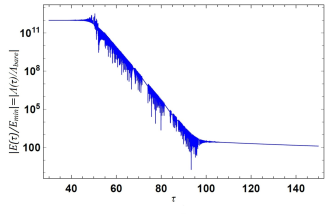
Using the above derived formulae one can find numerically within the model considered the survival probability ${\cal P}(t)$ and $\kappa(\tau(t))$ describing the behavior of the instantaneous energy $E(t)$. Results of these calculations performed for chosen $\beta$ are presented in Figs (1(a)), (1(b)).

From the results of the previous Section and those presented above and also in Fig (1(b)) it follows that a behavior of the instantaneous energy $E(t)$ and the instantaneous decay rate ${\it\Gamma}(t)$ differ depending on the time domain in which we examine their values. At canonical decay times $0\ll t<T_{1}$ they are close to a good approximation to the values resulting from the Weisskopf–Wigner theory of spontaneous emission. For times $t>T_{2}$ their behavior is described by late time asymptotic formulae (20) and (21). At transition time region of times $T_{1}<t<T_{2}$ the instantaneous energy $E(t)$ and the instantaneous decay rate ${\it\Gamma}(t)$ decrease to their late time asymptotic forms. Unfortunately the information of how fast $E(t)$ tends to its asymptotic form (20) at times $t>T_{1}$ is invisible in $\kappa(\tau(t))$ — see Fig (1(b)). In order to remove this deficiency one should come back to the Eq. (37). Namely by manipulating Eqs (37) — (39) we get the desired result,

$$\frac{E(\tau(t))}{E_{{min}}}=1+\left(\frac{E_{0}}{E_{{min}}}-1\right)\,\kappa(\tau(t)).$$

(40)

This last equation can be used to show how fast $E(t)$ tends to its asymptotic form (20) at times $t>T_{1}$ for assumed $\beta$ and the ratio $\frac{E_{0}}{E_{{min}}}$. Results obtained for $\omega(E)=\omega_{BW}(E)$ are presented in graphical form in Figs (1), (2), (3) and Fig (4).

We show now that similar results can be obtained not only in the approximate case $\omega_{BW}(E)$ of the density of the energy (mass) distribution $\omega(E)$ but also when one considers a more general forms of $\omega(E)$. As it was mentioned $\omega(E)$ should have a form given by Eq. (25), where the simple pole contribution, $P(E)$, is often modeled by $\omega_{BW}(E)$.

Guided by this observation we follow [60, 61] and assume that

$$\begin{split}\omega_{\eta}(E)&=N\,\sqrt{E-E_{min}}\,\times\\ &\times\frac{{\sqrt{{\it\Gamma}_{0}}}}{({E}-{E}_{0})^{2}+({{\it\Gamma}_{0}}/{2})^{2}}\,e^{\textstyle{-\eta\,\frac{E-E_{0}+E_{min}}{\it\Gamma_{0}}}},\end{split}$$

(41)

with $\eta>0$. Inserting this $\omega_{\eta}(E)$ into (5) we can calculate the survival amplitude ${\cal A}(t)$ for this case and then the effective Hamiltonian $h(t)$ and thus $E(t)$ that we want to study. Analogously to the above analyzed case of the Breit–Wigner energy density distribution, $\omega_{BW}(E)$, we get

$$\frac{E(\tau)-E_{min}}{E_{0}-E_{min}}=\kappa_{\eta}(\tau),$$

(42)

where

$$\kappa_{\eta}(\tau)=1+\;+\frac{1}{\beta}\,\Re\left[\frac{{\cal J}_{\beta}^{\eta}(\tau)}{{\cal I}_{\beta}^{\eta}(\tau)}\;\right].$$

(43)

and

	$\displaystyle{\cal J}_{\beta}^{\eta}$	$\displaystyle=$	$\displaystyle\int_{-\beta}^{\infty}\frac{x\sqrt{x+\beta}}{{x}^{2}+\frac{1}{4}}\,e^{\textstyle{-x\,\eta}}\,e^{\textstyle{-ix\tau}}\,dx,$		(44)
	$\displaystyle{\cal I}_{\beta}^{\eta}$	$\displaystyle=$	$\displaystyle\int_{-\beta}^{\infty}\frac{\sqrt{x+\beta}}{{x}^{2}+\frac{1}{4}}\,e^{\textstyle{-x\,\eta}}\,e^{\textstyle{-ix\tau}}\,dx.$		(45)

After some algebra, analogously to the result (40), we obtain the following relation in the considered here case:

$$\frac{E(\tau(t))}{E_{{min}}}=1+\left(\frac{E_{0}}{E_{{min}}}-1\right)\,\kappa_{\eta}(\tau(t)).$$

(46)

This equation, similarly to the Eq (40), can be used to show how fast $E(t)$ tends to its asymptotic form (20) at times $t>T_{1}$ for assumed $\omega(E)$, and for chosen $\beta$, $\eta$ and the ratio $\frac{E_{0}}{E_{{min}}}$. Results obtained for $\omega(E)=\omega_{\eta}(E)$ are presented graphically in Fig (5) — Fig (9).

In previous Sections we used the Krylov–Fock theory of unstable states to find late time properties of the survival amplitude and instantaneous energy. Similar estimations of the late time behavior of the survival amplitude can be also found by means another method, e.g. methods of the quantum scattering theory. This method was used in [63], where the long time deviations from the exponential form of the decay law were also studied and where one can find attempts to estimate the value of $T_{1}$. Newton on page 624 in Chap. 19 of [63] writes:

Let us now take some simple examples. Consider the case of a nuclear deexcitation by $\gamma$–ray emission. In a typical instance the energy may be $E_{0}\sim 200$ keV and the lifetime $\tau\sim 10^{-8}$ sec so that $\Gamma/E_{0}\sim 3\times 10^{-13}$. …. ………… The decay curve should be roughly exponential after 1/8 of a mean life from the peak and excellently exponential after 2. It then remains exponential for $10^{17}$ lifetimes! In order to destroy most of the exponential–decay curve, one would have to move the detector away to a distance of about $10^{22}$ miles. …………..

Note that $10^{22}$ miles equals $1.7\times 10^{9}$ light years approximately, so the effect described by Newton and in other papers should be visible when analyzing the spectrum of the electromagnetic radiation emitted by cosmic objects at a distance of $1.7\times 10^{9}$ light years or more from the Earth’s observer. Of course in this case it is practically impossible to restore the late time form of the decay curve by means measurements but as it has already been shown for times $t>T_{1}$ the following quantum effect should take place during the late time phase of the quantum decay process: The energy of the system in the initial metastable state, which is approximately equal $E_{0}$ at canonical decay times, is forced to decrease as $1/t^{2}$ to the minimal energy $E_{min}<E_{0}$. This effect was described in previous sections and earlier in [17, 18, 19, 20, 21, 64]. In the case of the emission of the electromagnetic radiation the excited atomic level can be considered as an the initial metastable state of the system. (In Newton’s example the excited state of a nucleus is the initial state). So, in the case of very distant cosmic objects emitting electromagnetic radiation this effect should contribute into the redshift making it apparently larger than it really is. Such a possibility seems to be very important as this effect may distort the observational results (red shift, luminosity, and so on) and thus lead to wrong conclusions (For example estimations of a tension of the Hubble parameter are based on the measurements of the red shift of distant astrophysical objects, etc.). Possible changes of the red shift caused by this possible effect are described in details in [17] (see also [64]), where an influence of this property on measured values of possible deviations of the fine structure constant $\alpha$ as well as other astrophysical and cosmological parameters were studied and this is why this is only signalized here.

Let us analyze now results presented in Fig (1(c)), Fig (2) — Fig (9). In Figure (1(c)), in contrast to Figure (1(b)), it can be seen how quickly in the transition time region, $T_{1}<t<T_{2}$, the energy $E(t)$ is reduced to its late time asymptotic form, $E_{lt}(t)=E_{min}+\alpha_{2}/t^{2}+\ldots$. Namely, if to compare Fig (1(c)), Fig (3) — Fig (9) and Fig (2(a)) a conclusion can be drawn that at transition times $T_{1}<t<T_{2}$ the instantaneous energy $E(t)$, (where $E(t)\simeq E_{0}$ for times $t<T_{1}$ and $t>T_{0}$), decreases like an oscillatory modulated exponential function until reaching its asymptotic form $E_{lt}(t)$. This quantum effect is very strong and efficient: As can be seen from Fig (1(c)), Fig (3) — Fig (9), the reduction of energy $E(t)\simeq E_{0}$ (for $t<T_{1}$) depending on the values of parameters $\beta$ and $\eta$, may be more than 10 orders: It can be $E(T_{1})/E_{lt}(T_{2})\sim 10^{12}$ — see Fig (3(d)), Fig (9(a)), and more. By selecting the appropriate parameters $\beta$ in $\omega_{BW}(E)$, or $\beta$ and $\eta$ in $\omega_{\eta}(E)$, or the other, more appropriate, energy density distribution function $\omega(E)$, even much greater reduction of the energy $E(t)\simeq E_{0}$ can be achieved when time $t$ runs from $t=T_{1}$ to $t=T_{2}$. Potentially, this effect can reduce the energy by tens of orders or more. Taking this property into account it seems to be reasonable to hypothesize that this quantum effect can help to explain the cosmological constant problem, which is consequence of the interpretation of the dark energy as the vacuum energy: The observed present value of the cosmological constant is 120 orders of magnitude smaller than we expect from quantum physics calculations.

One can meet in the large literature cosmological models with metastable vacuum (see, eg. [65, 66, 67, 68] and many others). Some of these models admit the lifetime of the Universe to be very small [66] or even smaller than the Planck time (see [67, 68]). Of course this decaying vacuum is described by the quantum state corresponding to a local minimum of the energy density which is not the absolute minimum of the energy density of the system considered. In such a case the formalism described in this paper is fully applicable. Let us consider now a cosmological scenario in which the lifetime of the false vacuum is shorter than the duration of the inflation phase and its decay process began before (or just before) the beginning of the inflation phase and then it is continued during the inflationary epoch and later. This scenario corresponds with the hypothesis analyzed by Krauss and Dent [22, 23]. Their hypothesis suggests that some false vacuum regions do survive well up to the time $T_{1}$ or later. So, let $|\phi\rangle=|0\rangle^{\text{F}}$ be a false and $|0\rangle^{\text{T}}$ true vacuum states, respectively, and $E_{0}=E^{\,{\text{F}}}_{0}$ be the energy of a state corresponding to the false vacuum measured at the canonical decay times, which leads to the vacuum energy density calculated using quantum field theory methods. Let $E^{\,\text{T}}=E_{min}$ be the energy of true vacuum (i.e., the true ground state of the system). The fact that the decay of the false vacuum is the quantum decay process [3, 4, 22, 23, 69] means that state vector corresponding to the false vacuum is a quantum unstable (or metastable) state. Therefore all the general properties of quantum unstable systems must also occur in the case of such a quantum unstable state as the false vacuum. This applies in particular to such properties as late time deviations from the exponential decay law and properties of the energy $E(t)=E^{\,\text{F}}(t)$ of the system in the quantum false vacuum state. In [20] it was pointed out the energy of those false vacuum regions which survived up to $T_{1}$ and much later differs from $E^{\,\text{F}}_{0}$.

If one wants to generalize the above results obtained on the basis of quantum mechanics to quantum field theory one should take into account among others a volume factors so that survival probabilities per unit volume should be considered and similarly the energies and the decay rate: $E\mapsto\rho(E)=\frac{E}{V_{0}}$, ${\it\Gamma}_{0}\mapsto\gamma=\frac{{\it\Gamma}_{0}}{V_{0}}$, where $V_{0}=V(t_{0}^{init})$ is the volume of the considered system at the initial instant $t_{0}^{init}$, when the time evolution starts. The volume $V_{0}$ is used in these considerations because the initial unstable state $|\phi\rangle\equiv|0\rangle^{\text{F}}$ at $t=t_{0}^{init}=0$ is expanded into eigenvectors $|E\rangle$ of $\mathfrak{H}$, (where $E\in\sigma_{c}(\mathfrak{H})$), and then this expansion is used to find the density of the energy distribution $\omega(E)$ at this initial instant $t_{0}^{init}$. Now, if we identify $\rho_{{de}}(t_{0}^{init})$ with the energy $E_{0}^{\;\text{F}}$ of the unstable system divided by the volume $V_{0}$: $\rho_{{de}}(t_{0}^{init})\equiv\rho_{0}^{\,\text{F}}\equiv\rho_{0}^{{qft}}\stackrel{{\scriptstyle\rm def}}{{=}}\rho_{{de}}^{0}=\frac{E_{0}^{\,\text{F}}}{V_{0}}$ and $\rho_{{bare}}=\frac{E_{{min}}}{V_{0}}$, (where $\rho_{{0}}^{{qft}}$ is the vacuum energy density calculated using quantum field theory methods) then it is easy to see that the mentioned changes $E\mapsto\frac{E}{V_{0}}$ and ${\it\Gamma}_{0}\mapsto\frac{{\it\Gamma}_{0}}{V_{0}}$ do not changes the parameter $\beta$:

$$\beta=\frac{E_{0}^{\,\text{F}}-E_{{min}}}{{\it\Gamma}_{0}}\equiv\frac{\rho_{de}^{0}-\rho_{bare}}{{\gamma}_{0}}>0,$$

(47)

(where $\gamma_{0}={\it\Gamma}_{0}/V_{0}$, or equivalently, ${\it\Gamma}_{0}/V_{0}\equiv\frac{\rho_{de}^{0}-\rho_{bare}}{\beta}$). This means that the relations (20), (35), (37), (40), (42), (43), (46) can be replaced by corresponding relations for the densities $\rho_{{de}}$ or $\Lambda$ (see, eg., [21, 32, 70, 71]). Simply, within this approach $E(t)=E^{\,\text{F}}(t)$ corresponds to the running cosmological constant $\Lambda(t)$ and $E_{{min}}$ to the $\Lambda_{bare}$. For example, we have

$$\begin{split}\kappa(t)&=\frac{E^{\,\text{F}}(t)-E_{{min}}}{E_{0}^{\,\text{F}}-E_{{min}}}\equiv\frac{\frac{E^{\,\text{F}}(t)}{V_{0}}-\frac{E_{{min}}}{V_{0}}}{\frac{E_{0}^{\,\text{F}}}{V_{0}}-\frac{E_{{min}}}{V_{0}}}\\ &=\frac{\rho^{F}(t)-\rho_{bare}}{\rho^{F}_{0}-\rho_{{bare}}}=\frac{\rho_{{de}}(t)-\rho_{{bare}}}{\rho_{{de}}^{0}-\rho_{{bare}}}\\ &=\frac{\Lambda(t)-\Lambda_{{bare}}}{\Lambda_{0}-\Lambda_{{bare}}}.\end{split}$$

(48)

and similarly,

$$\frac{E^{\,\text{F}}(t)}{E_{min}}=\frac{\Lambda(t)}{\Lambda_{bare}},\;\;\;\frac{E_{0}^{\,\text{F}}}{E_{min}}=\frac{\Lambda_{0}}{\Lambda_{bare}},$$

(49)

etc. Here $\rho^{F}(t)=\frac{E^{\,\text{F}}(t)}{V_{0}}\equiv\rho_{{de}}(t)$, $\Lambda(t)=\frac{8\pi G}{c^{2}}\,\rho_{de}(t)$, (or $\Lambda(t)=8\pi G\,\rho_{de}(t)$ in $\hbar=c=1$ units), etc. Equivalently, $\rho_{de}(t)=\frac{c^{2}}{8\pi G}\Lambda(t)$.

References

- [1] V. F. Weisskopf, E. T. Wigner, Berechnung der natürlichen Linienbreite auf Grund der Diracschen Lichttheorie, Z. Phys. 63, 54, (1930); Über die natürliche Linienbreite in der Strahlung des harmonischen Oszillators, Zeit. f. Phys., 65, 18, (1930).
- [2] G. Gamow, Zur Quantentheorie des Atomkernes, Zeit. f. Phys. 51, 204 —212, (1928).
- [3] S. R. Coleman, The fate of the false vacuum. 1. Semiclassical theory, Phys. Rev. D15 2929, (1977).
- [4] C. G. Callan, Jr. and S. R. Coleman, The fate of the false vacuum. 2. First quantum corrections, Phys. Rev. D16, 1762, (1977).
- [5] E. Ruthheford, Radioactivity produced in substances by the action of thorium compounds, Philosophical Magazine XLIX, 1, 161, (1900).
- [6] E. Rutherford, F. Soddy,The cause and nature of radioactivity. –Part I, Philosophical Magazine IV, 370––396, (1902); The cause and nature of radioactivity. –Part II, Philosophical Magazine IV, 569 — 585, (1902).
- [7] E. Rutherford, Radioactive substances and their radiations, Cambridge Unversity Press 1913.
- [8] L. A. Khalfin, Contribution to the decay theory of a quasi-stationary state, Zh. Exp. Teor. Fiz. 33 1371, (1957) .
- [9] L. Fonda, G. C. Ghirardi and A. Rimini, Decay Theory of Unstable Quantum Systems, Rept. Prog. Phys. 41 587, (1978).
- [10] M. Peshkin, A. Volya and V. Zelevinsky, Non-exponential and oscillatory decays in quantum mechanics, Europhys. Lett. 107, 40001, (2014).
- [11] B. Misra and E. C. G. Sudarshan, The Zeno’s paradox in quantum theory, J. Math. Phys. 18, 756 – 763 (1977).
- [12] A. Beige and G. C. Hegerfeldt, Projection postulate and atomic quantum Zeno effect, Phys. Rev. A, 53, 53, (1996).
- [13] A. Beige, G. C. Hegerfeldt and D. G. Sondermann, Atomic Quantum Zeno Effect for Ensembles and Single Systems, Foundations of Physics, 27, 1671 — 1688, (1997).
- [14] K. Koshinoa, A. Shimizuc, Quantum Zeno effect by general measurements, Physics Reports, 412, 191 – 275, (2005).
- [15] P. Facchi and S. Pascazio, Quantum Zeno Phenomena: Pulsed versus Continuous Measurement, Fortschr. Phys., 49, 941 – 947, (2001).
- [16] W. M. Itano, et al, Quantum Zeno effect, PhysicaL Review A, 41, 2295 – 2300, (1990); M. C. Fischer, B. Gutiérrez–Medina, and M. G. Raizen, Observation of the Quantum Zeno and Anti–Zeno Effects in an Unstable System, Physical Review Letters, 87, 040402, (2001); Wenqiang Zheng, D. Z. Xu, Xinhua Peng, Xianyi Zhou, Jiangfeng Du, and C. P. Sun, Experimental demonstration of the quantum Zeno effect in NMR with entanglement-based measurements, Physical Review A, 87, 032112, (2013); Erik W. Streed, et al, Continuous and Pulsed Quantum Zeno Effect, Physical Review Letters, 97, 260402, (2006); Y. S. Patil, S. Chakram, and M. Vengalattore, Measurement-Induced Localization of an Ultracold Lattice Gas, Physical Review Letters, 115, 140402, (2015); A. Signoles, et al, Confined quantum Zeno dynamics of a watched atomic arrow, Nature Physics, 10, 715 – 719, (2014).
- [17] K. Urbanowski, A quantum long time energy red shift: A contribution to varying alpha theories, Eur. Phys. J. C58 151, (2008).
- [18] K. Urbanowski, General properties of the evolution of unstable states at long times, Eur. Phys. J. D54, 25, (2009).
- [19] K. Urbanowski, Long time properties of the evolution of an unstable state, Cent. Eur. J. Phys. 7, 696, (2009).
- [20] K. Urbanowski, Comment on ‘Late time behavior of false vacuum decay: Possible implications for cosmology and metastable inflating states’, Phys. Rev. Lett. 107, 209001, (2011).
- [21] K. Urbanowski, Properties of the false vacuum as the quantum unstable state, Theor. Math., 458, Phys. 190 (2017).
- [22] L. M. Krauss and J. Dent, The late time behavior of false vacuum decay: Possible implications for cosmology and metastable inflating states, Phys. Rev. Lett. 100, 171301, (2008).
- [23] L. M. Krauss, J. Dent and G. D. Starkman, Late time decay of the false vacuum, measurement, and quantum cosmology, Int. J. Mod. Phys. D17, 2501, (2009).
- [24] Ta–Pei Cheng, Relativity, Gravitation, and Cosmology: A basic introduction, Oxford University Press, 2005.
- [25] S. Weinberg, Cosmology, Oxford University Press, 2008.
- [26] R. G. Landim and E. Abdalla, Metastable dark energy, Phys. Lett., B764, 271 — 276, (2017).
- [27] D. Stojkovic, Glenn D. Starkman, and Reijiro Matsuo, Dark energy, colored anti–-de Sitter vacuum, and the CERN Large Hadron Collider phenomenology, Physical Review, D 77, 063006, (2008).
- [28] J.A.S. Lima, Extended metastable dark energy, Physics of the Dark Universe, 30, 100713, 2020.
- [29] A. Stachowski1, M. Szydłowski1, K. Urbanowski, Cosmological implications of the transition from the false vacuum to the true vacuum state, Eur. Phys. J. C 77, 357, (2017).
- [30] M. Szydlowski, A. Stachowski and K. Urbanowski, Quantum mechanical look at the radioactive-like decay of metastable dark energy, Eur. Phys. J. C77, 902, (2017).
- [31] M. Szydlowski and A. Stachowski, Cosmological models with running cosmological term and decaying dark matter, Phys. Dark Univ. 15, 96, (2017).
- [32] M. Szydłowski, A. Stachowski and K. Urbanowski, The evolution of the FRW universe with decaying metastable dark energy — a dynamical system analysis, Journal of Cosmology and Astroparticle Physics, 04 029 (2020).
- [33] N. S. Krylov and V. A. Fock, On two main interpretations of energy-time uncertainty, Zh. Eksp. Teor. Fiz. 17, 93, (1947).
- [34] V. A. Fock, Fundamentals of Quantum Mechanics. Mir Publishers, Moscow, 1978.
- [35] N. G. Kelkar and M. Nowakowski, No classical limit of quantum decay for broad states, J. Phys. A43, 385308, (2010).
- [36] F. Giacosa, Non-exponential decay in quantum field theory and in quantum mechanics: the case of two (or more) decay channels, Found. Phys. 42, 1262, (2012).
- [37] F. Giacosa, QFT derivation of the decay law of an unstable particle with nonzero momentum, Adv. High Energy Phys. 2018, 4672051, (2018).
- [38] R. E. A. C. Paley, N. Wiener, Fourier transforms in the complex domain, American Mathematical Society, New York, 1934.
- [39] A. Peres, Nonexponential decay law Ann. Phys. 129, 33, (1980).
- [40] K. M. Sluis and E. A. Gislason, Decay of a quantum-mechanical state described by a truncated Lorentzian energy distribution, Phys. Rev. A43, 4581, (1991).
- [41] M. L. Goldberger, K. M. Watson, Collision Theory, Willey, New York 1964.
- [42] D. G. Arbo, M. A. Castagnino, F. H. Gaioli and S. Iguri, Minimal irreversible quantum mechanics.The decay of unstable states, Physica, A 227, 469 — 495, (2000).
- [43] J. M. Wessner, D. K. Andreson and R. T. Robiscoe, Radiative Decay of the 2P State of Atomic Hydrogen: A Test of the Exponential Decay Law, Phys. Rev. Lett. 29, 1126 — 1128, (1972).
- [44] E. B. Norman, S. B. Gazes, S. C. Crane and D. A. Bennet, Tests of the Exponential Decay Law at Short and Long Times, Phys. Rev. Lett., 60, 2246 — 2249, (1988).
- [45] P. T. Greenland, eeking non-exponential decay, Nature 335, 298, (1988).
- [46] J. Seke, W. N. Herfort, Deviations from exponential decay in the case of spontaneous emission from a two–level atom, Phys. Rev. A 38, 833, (1988).
- [47] R. E. Parrot, J. Lawrence, Persistence of exponential decay for metastable quantum states at long times, Europhys. Lett. 57, 632 — 638, (2002).
- [48] J. Lawrence, Nonexponential decay at late times and a different Zeno paradox, Journ. Opt. B: Quant. Semiclass. Opt. 4, No 4, S446 — S449, (2002).
- [49] I. Joichi, Sh. Matsumoto, M. Yoshimura, Time evolution of unstable particle decay seen with finite resolution, Phys. Rev. D 58, 045004, (1998).
- [50] N. G. Kelkar, M. Nowakowski and K. P. Khemchandani, Hidden evidence of nonexponential nuclear decay, Phys. Rev. C 70, 024601, (2004).
- [51] M. Nowakowski, N. G. Kelkar, Long Tail of Quantum Decay from Scattering Data, AIP Conf. Proc. 1030, 250 — 255, (2008); arXiv: 0807.5103.
- [52] R. Santra, J. M. Shainline, Ch. H. Greene, Phys. Rev. Siegert pseudostates: Completeness and time evolution, A 71, 032703, (2005).
- [53] R. G. Winter, Evolution of a quasi-stationary state, Phys. Rev. 123, 1503, (1961).
- [54] T. Jiitoh, S. Matsumoto, J. Sato, Y. Sato, K. Takeda, Phys Rev. A 71, 012109, (2005).
- [55] C. Rothe, S. I. Hintschich and A. P. Monkman, Violation of the Exponential-Decay Law at Long Times, Phys. Rev. Lett. 96, 163601, (2006).
- [56] K. Urbanowski, Early-time properties of quantum evolution, Phys. Rev. A50, 2847, (1994).
- [57] F. Giraldi, Logarithmic decays of unstable states, Eur. Phys. J. D69, 5, (2015).
- [58] F. Giraldi, Logarithmic decays of unstable states II, Eur. Phys. J. D70, 229, (2016).
- [59] G. Breit and E. Wigner, Capture of Slow Neutrons, Phys. Rev. 49, 519–531, (1936).
- [60] N. G. Kelkar, M. Nowakowski, No classical limit of quantum decay for broad states, J. Phys. A: Math. Theor., 43, 385308, (2010).
- [61] D. F. Ramírez Jiménez and N. G. Kelkar, Formal aspects of quantum decay, Phys. Rev. A, 104, 022214, (2021).
- [62] K. Raczyńska and K. Urbanowski, Survival amplitude, instantaneous energy and decay rate of an unstable system: Analytical results, Acta Phys. Polon. B49, 1683, (2018).
- [63] R. G. Newton, Scattering Theory of Waves and Particles, Springer, New York 1982.
- [64] K. Urbanowski, K. Raczyńska, Possible emission of cosmic X- and ă -rays by unstable particles at late times, Physics Letters B, 731, 236 — 241, (2014).
- [65] J. Rubio, Higgs inflation and vacuum stability, J. Phys. Conf. Ser. 631, 012032, (2015).
- [66] A. Kennedy, G. Lazarides and Q. Shafi, Decay of the false vacuum in the very early universe, Phys. Lett. B99, 38, (1981).
- [67] V. Branchina and E. Messina, Stability, Higgs boson mass and new physics, Phys. Rev. Lett. 111, 241801, (2013).
- [68] V. Branchina, E. Messina and M. Sher, Lifetime of the electroweak vacuum and sensitivity to Planck scale physics, Phys. Rev. D91, 013003, (2015).
- [69] S. Winitzki, Age-dependent decay in the landscape, Phys. Rev. D 77, 063508, (2008).
- [70] K. Urbanowski, M. Szydlowski, Cosmology with a decaying vacuum, AIP Conf. Proc. 1514, 143, (2012).
- [71] M. Szydlowski, A. Stachowski, K. Urbanowski, Cosmology with a decaying vacuum energy parametrization derived from quantum mechani, Journal of Physics: Conference Series 626, 012033, (2015).
- [72] V. Sahni and A. Starobinsky, The Case for a Positive Cosmological –term, International Journal of Modern Physics D, 09, 373 — 443, (2000).
- [73] Vivian Poulin, Tristan L. Smith, Tanvi Karwal, and Marc Kamionkowski, Early Dark Energy can Resolve the Hubble Tension, Physical Review Letters, 122, 221301, (2019).
- [74] Tristan L. Smith, Vivian Poulin and Mustafa A. Amin, Oscillating scalar fields and the Hubble tension: A resolution with novel signatures, Physical Review D, 101, 063523, (2020).
- [75] Florian Niedermann and Martin S. Sloth, New early dark energy, Physical Review D, 103, L041303, (2021).
- [76] Vivian Poulin, Tristan L. Smith and Alexa Bartlett, Dark Energy at early times and ACT: a larger Hubble constant without late–time priors, arXiv: 2109.06229v1 [astro–ph.CO], (2021).
- [77] Eleonora Di Valentino, Olga Mena, Supriya Pan, Luca Visinelli, Weiqiang Yang, Alessandro Melchiorri, David F. Mota, Adam G. Riess and Joseph Silk, In the realm of the Hubble tension.a review of solutions, Class. Quantum Grav., 38, 153001, (2021)
- [78] Sunny Vagnozzi, Consistency tests of CDM from the early integrated Sachs–Wolfe effect: Implications for early-time new physics and the Hubble tension, Physical Review D, 104, 063524, (2021).
- [79] S. Weinberg, The cosmological constant problem, Rev. Mod. Phys. 61, 1, (1989).
- [80] S. Weinberg, The cosmological constant problems, in Sources and Detection of Dark Matter and Dark Energy in the Universe. Proceedings, 4th International Symposium, DM 2000, Marina del Rey, USA, February 23-25, 2000, pp. 18–26, 2000,
- [81] S. M. Carroll, The Cosmological Constant, Living Rev. Relativity,4, 1, (2001); arrXiv:astro-ph/0004075v2.
- [82] E. Di Valentino, E. V. Linder and A. Melchiorri, Vacuum phase transition solves the tension, Phys. Rev., D97, 043528, (2018).
- [83] Florian Niedermann and Martin S. Sloth, Resolving the Hubble tension with new early dark energy, Physical Review D, 102, 063527, (2020).
- [84] W. van Dijk and Y. Nogami, Novel expression for the wave function of a decaying quantum system, Phys. Rev. Lett. 83, 2867, (1999).
- [85] W. van Dijk and Y. Nogami, Analytical approach to the wave function of a decaying quantum system, Phys. Rev. C65, 024608, (2002).
- [86] D. A. Dicus, W. W. Rebko, R. F. Schwitters and T. M. Tinsley, Time development of a quasistationary state, Phys. Rev. A65, 032116, (2002).
- [87] J. Martorell, J. G. Muga and D. W. L. Sprung, Quantum post-exponential decay, in Time in Quantum Mechanics, Vol. 2, G. Muga, A. Ruschhaupt and A. del Campo, eds., vol. 789 of Lect. Notes Phys., (Berlin), pp. 239–275, Springer-Verlag, (2009),
- [88] W. van Dijk and F. M. Toyama, Decay of a quasistable quantum system and quantum backflow, Phys. Rev. A100, 052101, (2019).
- [89] I. L. Shapiro, J. Sola, C. Espana-Bonet and P. Ruiz-Lapuente, Variable cosmological constant as a Planck scale effect, Phys. Lett. B574, 149, (2003).
- [90] C. Espana-Bonet, P. Ruiz-Lapuente, I. L. Shapiro and J. Sola, Testing the running of the cosmological constant with type Ia supernovae at high z, JCAP 0402, 006, (2004).
- [91] A. H. Guth, Inflation, Proc. Nat. Acad. Sci. USA, 90, 4871 — 4877, (1993); Eternal inflation and its implications, J. Phys. A: Math. Theor. 40, 6811 — 6826, (2007).
- [92] J. M. Overduin and F. I. Cooperstock, Evolution of the scale factor with a variable cosmological term, Physical Review D, 58, 043506, (1998).
- [93] I. G. Dymnikova, M. Yu. Khlopov, Self-consistent initial conditions in inflationary cosmology, Gravitation & Cosmology, 4, Supplement; 50 — 55, (1988). I. G. Dymnikova, M. Yu. Khlopov, Decay of cosmological constant as Bose condensate evaporation, Mod. Phys. Lett. A . (2000) 15, 2305 — 2314, (2000); arXiv: astro-ph/0102094. I. G. Dymnikova, M. Yu. Khlopov, Decay of cosmological constant in self-consistent inflation Eur. Phys. J. C 20, 139 — 146, (2001). S. Ray, M. Yu. Khlopov, P. P. Ghosh and Utpal Mukhopadhyay, Phenomenology of -CDM model: a possibility of accelerating Universe with positive pressure, Int. J. Theor. Phys. (2011), 50, 939 — 951, (2011); arXiv: 0711.0686 [gr-qc].
- [94] K. Bamba, S. Capozziello, S. Nojiri and S. D. Odintsov, Dark energy cosmology: the equivalent description via different theoretical models and cosmography tests, Astrophys. Space Sci. 342, 155, (2012); [arXiv:1205.3421 [gr-qc]].
- [95] Elcio Abdalla, L. L. Graef, Bin Wang, A model for dark energy decay, Physics Letters B726, 786 — 790, (2013).