Correlations of Methyl Formate (CH3OCHO), Dimethyl Ether (CH3OCH3) and Ketene (H2CCO) in High-mass Star-forming Regions
Abstract
We present high-spatial-resolution (0.7 to 1.0 arcsec) submillimeter observations of continuum and molecular lines of CH3OCHO, CH3OCH3, and H2CCO toward 11 high-mass star-forming regions using the Atacama Large Millimetre/submillimetre Array (ALMA). A total of 19 separate cores from 9 high-mass star-forming regions are found to be line-rich, including high-, intermediate-, and low-mass line-rich cores. The three molecules are detected in these line-rich cores. We map the emission of CH3OCHO, CH3OCH3, and H2CCO in 9 high-mass star-forming regions. The spatial distribution of the three molecules is very similar and concentrated in the areas of intense continuum emission. We also calculate the rotation temperatures, column densities, and abundances of CH3OCHO, CH3OCH3, and H2CCO under the local thermodynamic equilibrium (LTE) assumption. The abundances relative to H2 and CH3OH, and line widths of the three molecules are significantly correlated. The abundances relative to H2, temperatures and line widths of the three molecules tend to be higher in cores with higher mass and outflows detected. The possible chemical links of the three molecules are discussed.
keywords:
Astrochemistry – ISM: molecules – star: formation1 Introduction
The astrochemical networks of many species have gradually been revealed. These species range from simple neutral molecules, molecular radicals, and ions to complex organic molecules (COMs). COMs are defined as C-bearing molecules with at least six atoms (Herbst & van Dishoeck, 2009). At present, two major pathways for producing organic molecules have been proposed: (i) grain-surface chemical reactions (Hasegawa et al., 1992; Ruffle & Herbst, 2000; Garrod et al., 2008; Ruaud et al., 2015); (ii) gas-phase chemical reactions (Duley & Williams, 1984; Vasyunin & Herbst, 2013; Balucani et al., 2015). Comparing the abundance and spatial distribution correlations of different species is an important mean to test chemical models and determine their formation paths. For example, interferometric observations showed a difference in the spatial distribution of O- and N-bearing molecules (Friedel & Snyder, 2008; Csengeri et al., 2019; Qin et al., 2015; Qin et al., 2022), with N-bearing molecules tracing higher temperature gas than O-bearing molecules (Qin et al., 2010; Crockett et al., 2015; van ’t Hoff et al., 2020). In particular, methyl formate (CH3OCHO) and dimethyl ether (CH3OCH3) were found to have a potential similarity (Jaber et al., 2014; Coletta et al., 2020; Peng et al., 2022; Chen et al., 2023). Nevertheless, the spatial similarity between CH3OCHO and CH3OCH3 has not been systematically confirmed by interferometric observations with large samples.
Ketene (H2CCO) has been proposed as an important precursor for the formation of COMs, such as acetic acid (CH3COOH), acetamide (CH3CONH2), pyruvonitrile (CH3COCN) and methyl acetate (CH3COOCH3) (Hudson & Loeffler, 2013). However, there are still many uncertainties about how this molecule is produced (Charnley & Rodgers, 2005; Ruiterkamp et al., 2007; Vasyunin & Herbst, 2013; Maity et al., 2014; Krasnokutski et al., 2017; Fedoseev et al., 2022). CH3OCHO, CH3OCH3, and H2CCO are commonly detected in the same sources of hot molecular cores (HMCs) (Nummelin et al., 2000; Belloche et al., 2013), hot corinos (Bergner et al., 2017; Jørgensen et al., 2018; Bergner et al., 2019; Agúndez et al., 2019) or cold regions (Bacmann et al., 2012; Cernicharo et al., 2012; Jaber et al., 2014). Previous models have also shown that there may be chemical associations among the three molecules (Garrod & Herbst, 2006; Garrod et al., 2008; Balucani et al., 2015; Charnley et al., 2001; Charnley & Rodgers, 2005). Whereas the relationship of H2CCO with the other two molecules has been barely explored from the observational side.
In this work, the correlations among CH3OCHO, CH3OCH3, and H2CCO are investigated toward 11 high-mass star-forming regions using Atacama Large Millimeter/submillimeter Array (ALMA) data. These data were observed as a pilot project for the ALMA Three-millimetre Observations of Massive Star-forming regions (ATOMS) survey (Liu et al., 2020). These 11 targets have large masses and luminosity (Xu et al., 2024), and show infall motion traced by the “blue profiles” observed by the HCN (4-3) lines (Liu et al., 2016). The paper is organized as follows. The observations and data reduction are described in Section 2. The observational results including continuum, line identifications, parameter calculation, and molecular emission maps are given in Section 3. We discuss the correlations of the three molecules and their implications for chemistry in Section 4. The main results and conclusions are summarized in Section 5.
2 Observations
The basic observational parameters and data reduction are described in Chen et al. (2024). Observations of 11 high-mass star-forming regions were performed from 18 to 20 May 2018 under the ALMA Cycle 5 project at Band 7 (ID: 2017.1.00545.S, PI: Tie Liu). A total of 43 antennas with a diameter of 12m were employed for observations (C43-1 configuration). The Band 7 observations offer 4 spectral windows (SPWs) centering at the frequency of 343.2 (SPW 31), 345.1 (SPW 29), 345.4 (SPW 25), and 356.7 GHz (SPW 27), respectively. Both SPWs 25 and 27 have a bandwidth of 469 MHz and a spectral resolution of 0.24 km s-1, and are used to observe HCN (4-3) and HCO+ (4-3) lines, respectively. In this paper, we present the spectral line data of SPW 29 and SPW 31, both having a bandwidth of 1.88 GHz with a velocity resolution of 0.98 km s-1. We used the TCLEAN task in Common Astronomy Software Applications (CASA; McMullin et al. 2007) to generate images of continuum and spectral cubes. Before the imaging processes, the bandpass, amplitude, and phase calibration were performed by running “ScriptForPI.py” offered by the ALMA team. For I14498, the phase calibrator is J1524-5903, and the flux and bandpass calibrator is J1427-4206. For I17220, the phase calibrator is J1733-3722, and the flux and bandpass calibrator is J1924-2914. As for the other 7 sources, the phase calibrator is J1650-5044, and the flux and bandpass calibrators are J1924-2914, J1427-4206, and J1517-2422. The continuum image was constructed from all line-free channels of four spectral windows. Self-calibrations were performed to improve the qualities of continuum images. Totally 3 rounds of phase self-calibrations and 1 round of amplitude self-calibration had been conducted to all continuum data of 11 sources. During the self-calibration, we used the “hogbom” deconvolution algorythm with a weighting parameter of “briggs”. The robust parameter of “briggs” weighting can be set from 2.0 to 2.0 to smoothly customize trade-offs between resolution and imaging sensitivity. The “robuts=0.5” was set to balance the sensitivity and resolution of our images. Following self-calibration, the Root-Mean-Square (rms) noise of the source I15520 was reduced by approximately 19%, the source I14498, I16351 and I17220 by about 3%, and the source I15596, I16060, I16076, I16272 and I17204 were barely improved. The primary beam correction had also been performed. Finally, the solutions from the self-calibration of continuum images were applied to line cubes. The synthesized beam sizes of continuum images and line cubes range from 0.7 to 1.0 arcsec. The average sensitivity is better than 8.0 mJy beam-1 per channel for line cubes, and better than 2.5 mJy beam-1 for continuum images.
3 Results
3.1 Continuum Emission
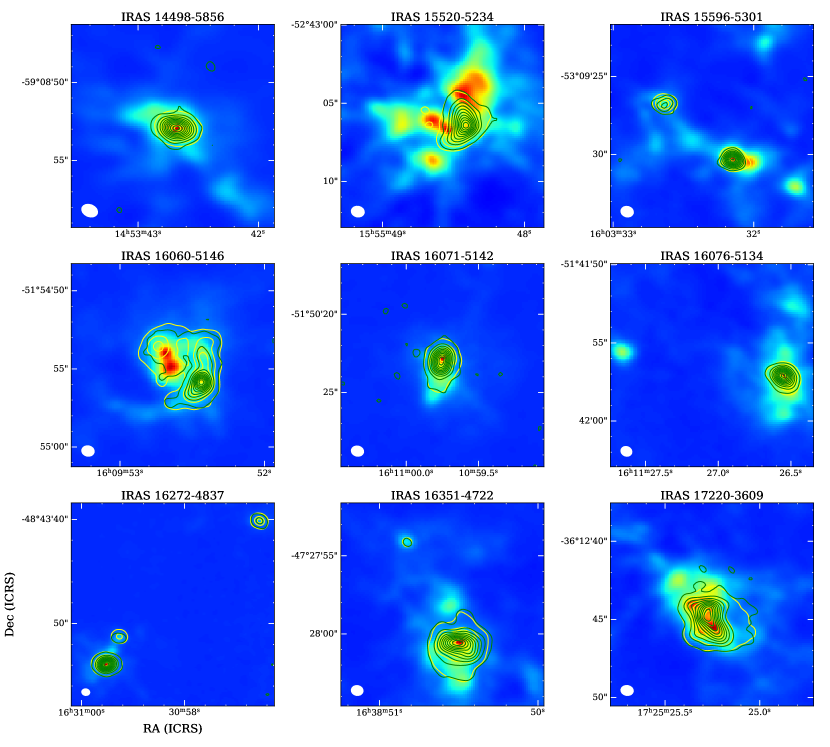
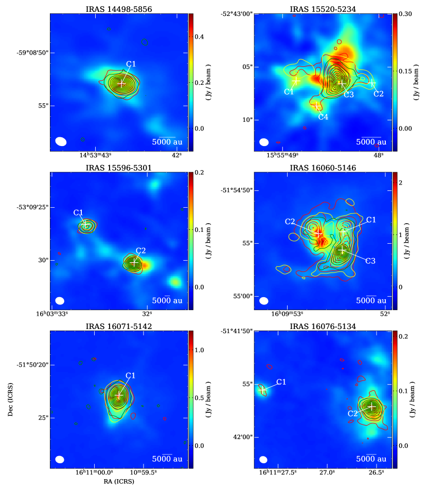
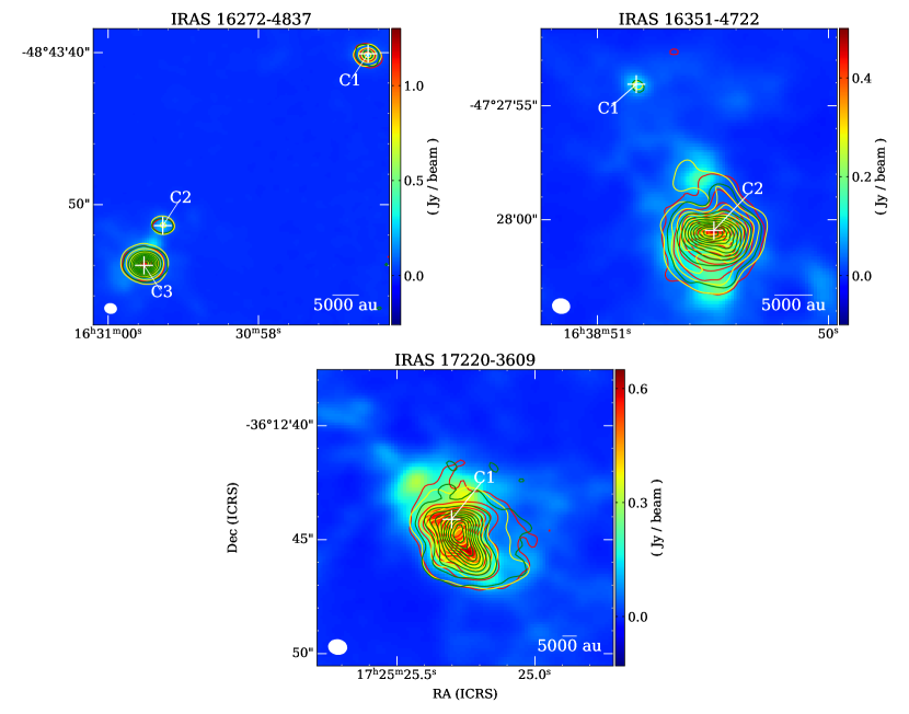
We perform multi-component two-dimensional Gaussian fits to 870 m continuum emission using the CASA- function. A total of 145 dense cores were resolved in 11 high-mass star-forming regions (Chen et al., 2024). We have checked the spectra towards the 145 cores one by one, and found that 19 separate cores in 9 regions have multiple line emissions of CH3OCHO or CH3OCH3 or H2CCO. From Figure 1 and 8, these 19 cores show rich line emission. The ALMA 870 m continuum emission from 9 high-mass star-forming regions is shown in Figure 2. The positions of 19 line-rich cores are labeled. For the other two of the 11 high-mass star-forming regions (IRAS 14382-6017 and IRAS 17204-3636), the line transitions of the three molecules were not detected. The absence of HMCs from these two sources was affirmative by cross-matching with the ALMA Band 3 dataset (Qin et al., 2022).
For the estimation of the core masses and the molecular hydrogen column densities, the commonly used method assumes that the dust emission is optically thin and in local thermodynamic equilibrium (LTE). Under these assumptions, the core masses and source-averaged H2 column densities can be estimated by the expressions (Kauffmann et al., 2008):
| (1) |
| (2) |
where Sν is integrated flux density, = 100 is gas-to-dust mass ratio (Lis et al., 1991; Hasegawa et al., 1992), D is the distance to the core (Liu et al., 2020) and the uncertainty takes 10% (Baug et al., 2020; Liu et al., 2022) when calculating the uncertainty of the core mass, ν is the dust mass absorption coefficient, Bν(T) is the Planck function at dust temperature T, = 2.8 is the mean molecular weight of the gas (Kauffmann et al., 2008), mH is the mass of the hydrogen atom, and is the solid angle corresponding to the deconvolved size of the core. In our case, 870μm takes a value of 1.89 cm2 g-1, which is interpolated from the table given in Ossenkopf & Henning (1994), assuming grains with thin ice mantles and a gas density of 106 cm-3. The dust temperatures of dense cores are assumed to be the rotation temperatures of CH3OCHO, which is considered to be dust temperature probe (Favre et al., 2011). The parameters of 19 line-rich cores are listed in Table 1. In Table 1, we also list whether these cores are associated with outflows. The presence of outflows is identified by searching for red-blue lobes around continuum sources using the CO (3-2), HCN (4-3), and SiO (2-1) lines (Baug et al., 2020).
The source-averaged optical depths of the continuum can be calculated by the following formula (Frau et al., 2010; Gieser et al., 2021):
| (3) |
The derived 870μm ranges from 6.2 × 10⁻³ to 1.4 × 10⁻¹ for the 19 dense cores, so the optically thin assumption is reasonable. I15520, I16060, I16071, I16076, I16351, and I17220 were found to be associated with the ultra-compact (UC) Hii regions traced by the H40 lines (Qin et al., 2022; Liu et al., 2022). Free-free emissions from UC Hii regions in the submillimeter band are weak, which have less contribution to the continuum flux.
3.2 Line Identifications
We extracted the spectra from the continuum peak positions of these dense cores. Then the spectral line transitions are identified using the eXtended CASA Line Analysis Software Suite (XCLASS111https://xclass.astro.uni-koeln.de; Möller et al. 2017). XCLASS searches for molecular line parameters in the Jet Propulsion Laboratory (JPL222http:///spec.jpl.nasa.gov; Pickett et al. 1998) and the Cologne Database for Molecular Spectroscopy (CDMS333http://cdms.de; Müller et al. 2001, 2005). The value of the partition functions in the XCLASS have 110 different temperature intervals between 1.072 and 1000 K. Assuming that the molecular gas satisfies the LTE condition, the XCLASS solves the radiative transfer equation and produces synthetic spectra for specific molecular transitions by taking into account beam dilution, dust attenuation, line opacity, and line blending. In the XCLASS modeling, the input parameters are the size (), rotational temperature (T), column density (N), line width (V), and velocity offset (Voff) of each molecule. In our study, we took the deconvolved sizes (see Table 1) of the continuum sources as molecular component sizes. To better fit the rotation temperature, column density, and line width parameters, we further employed Modeling and Analysis Generic Interface for eXternal numerical codes (MAGIX; Möller et al. 2013). The MAGIX optimizes these molecular component parameters within the given range and provides the corresponding error estimates. The parameter ranges are set based on the initial guesses provided by XCLASS fitting. Note that in our case the optical depths of the continuum cores are less than 1.4 × 10⁻¹ and then the dust attenuation effect can be ignored.
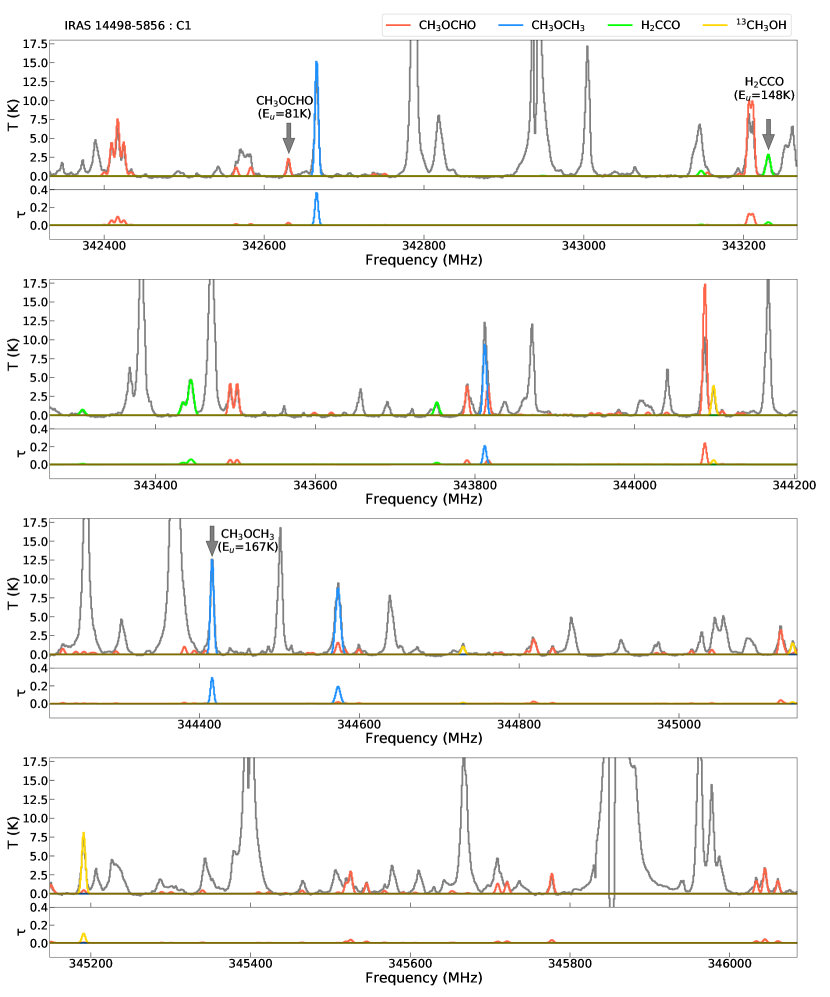
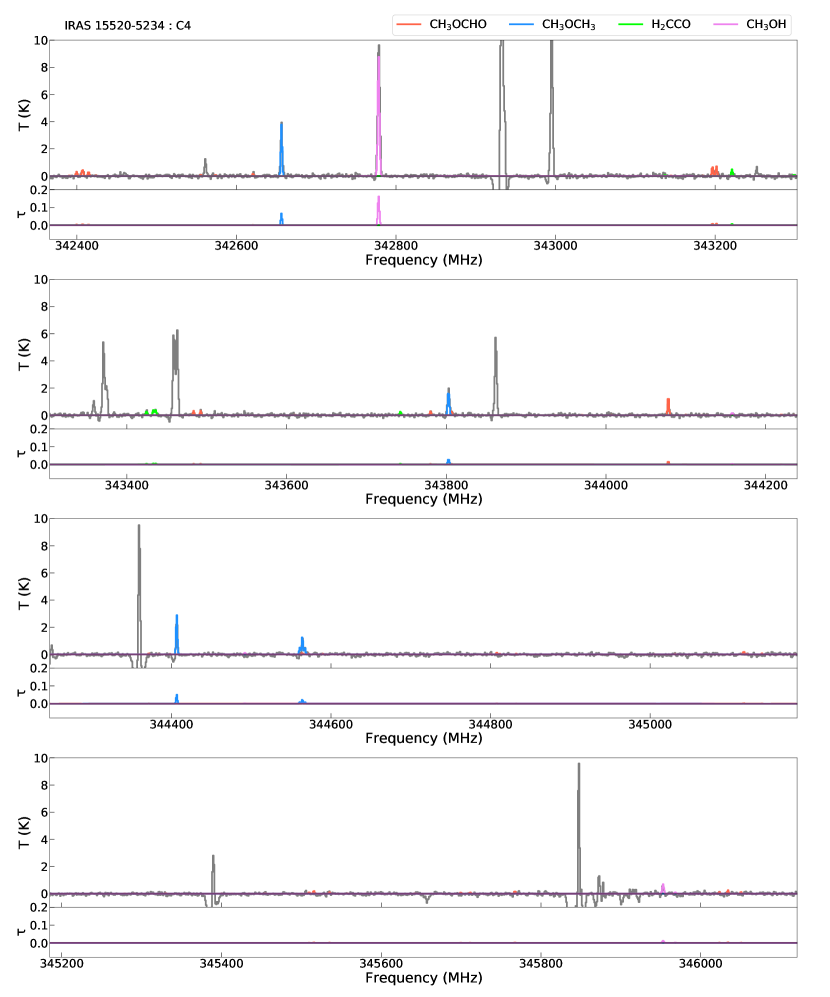
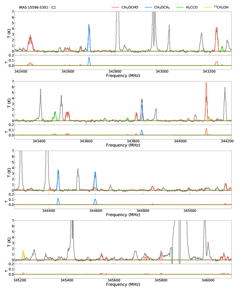
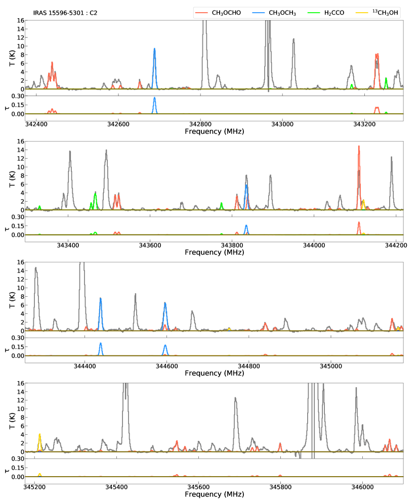
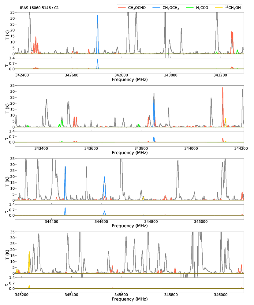
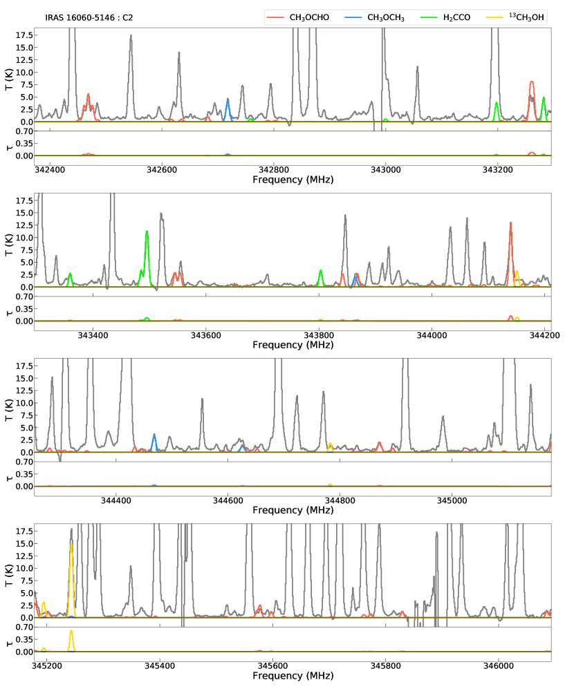
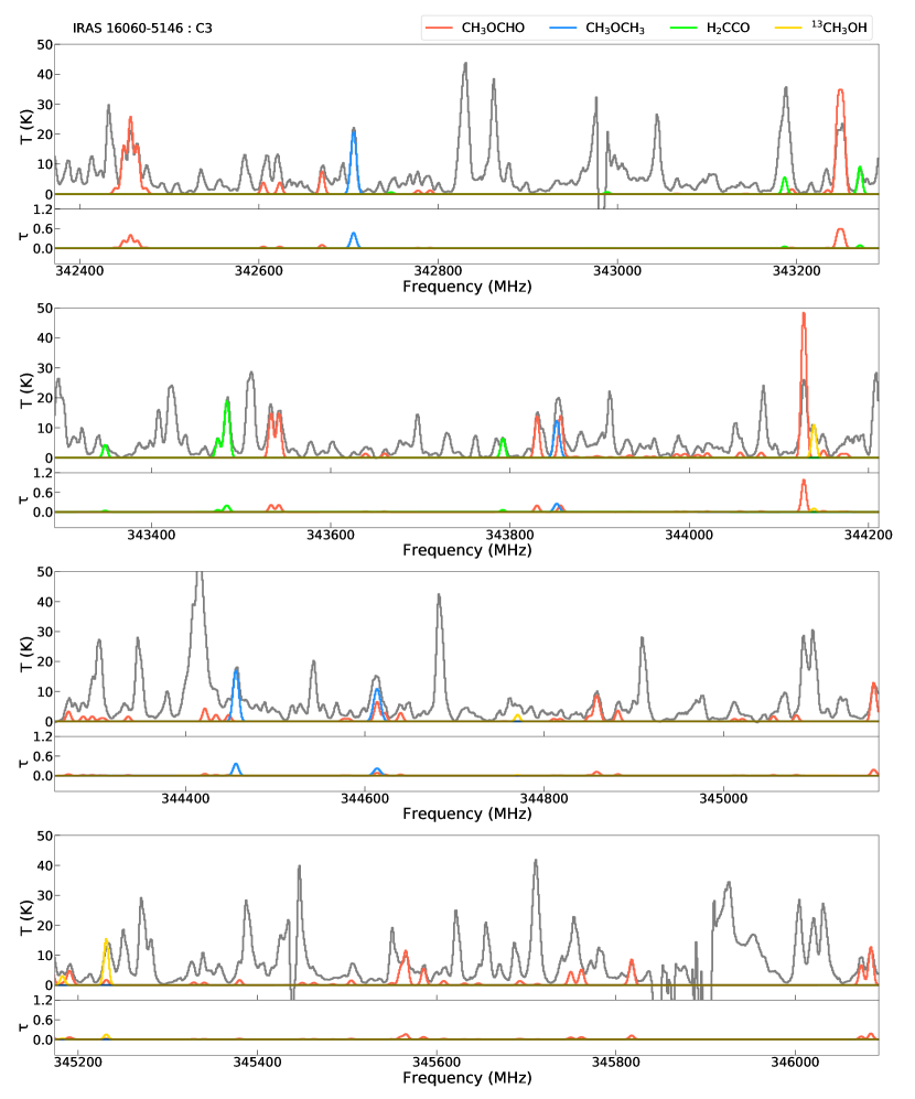
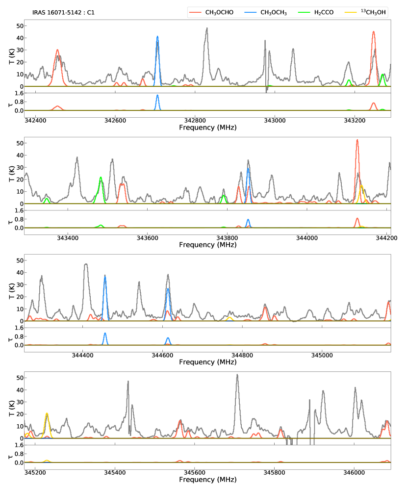
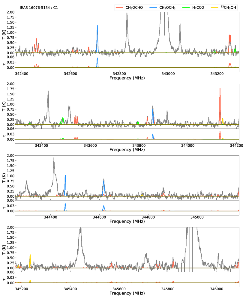
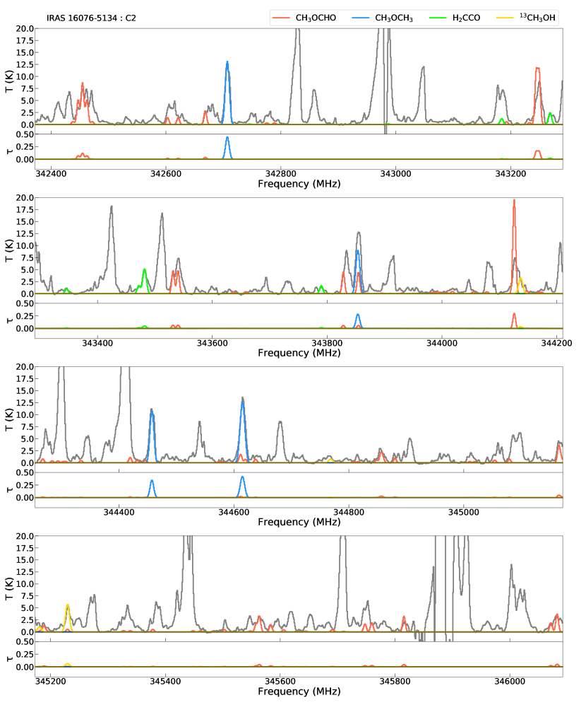
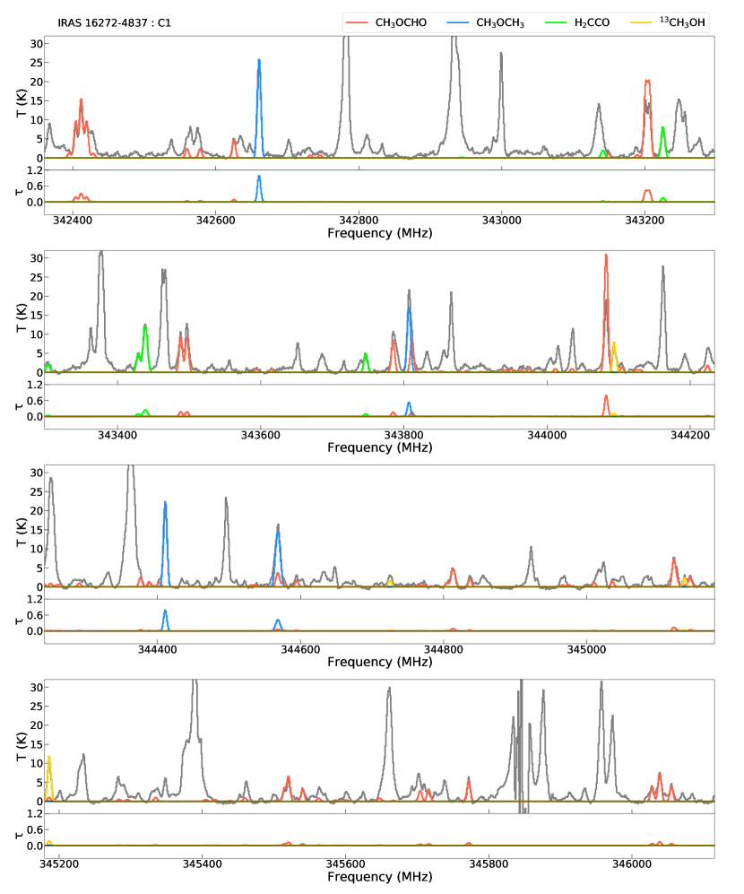
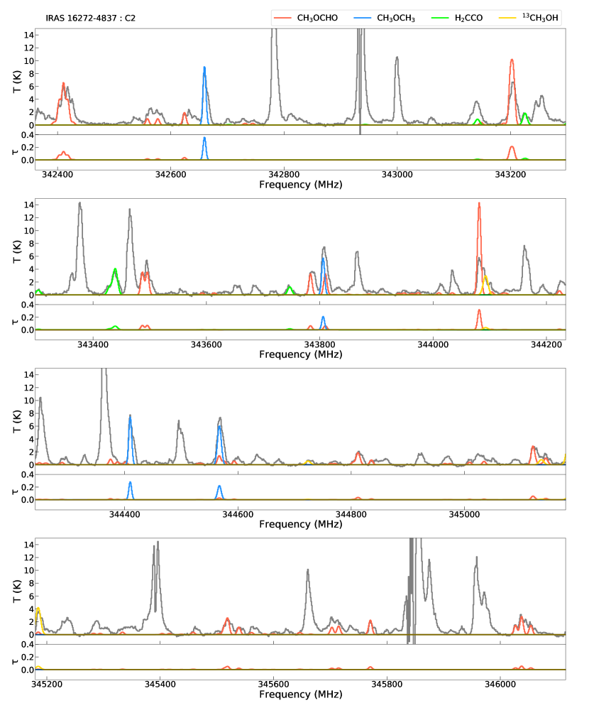
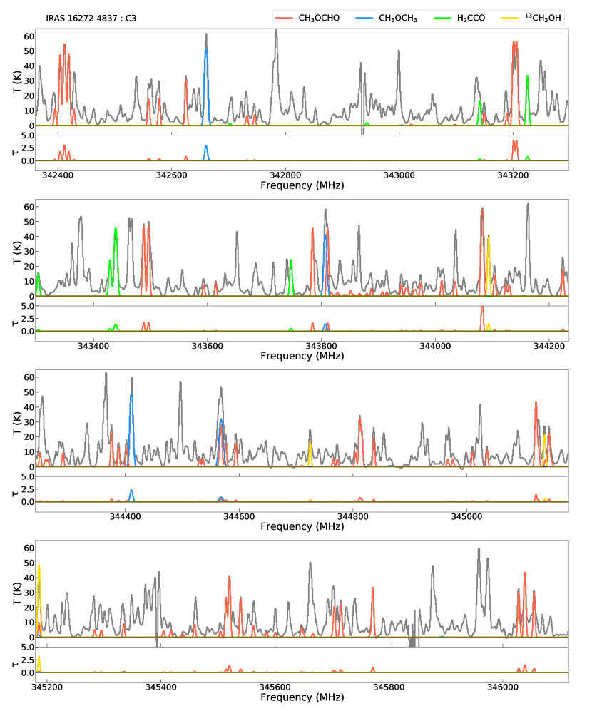
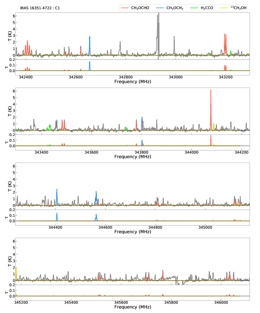
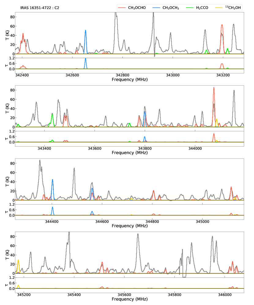
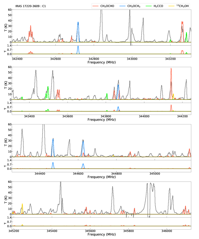
Transitions are considered as detection if the line intensities exceed 3 noise level. CH3OCHO, CH3OCH3, H2CCO, and CH3OH lines are detected in all 19 line-rich cores, and 13CH3OH lines are detected in 16 line-rich cores. Figure 1 shows the sample spectra and optical depths of molecular transitions toward I14498 C1. The spectra and optical depths of molecular transitions toward the other 18 cores are presented in Figure 8 of Appendix A. The overall results of the detected spectral lines are summarized as follows:
| Region | Core | D | R.A. | DEC. | dec | Rcore | Ipeak | Sν | T | Mcore | N (H2) | Outflows | Mass Classification |
| (kpc) | (h : m : s) | ( : : ) | maj() × min() | (au) | (mJy beam-1) | (mJy) | (K) | (M⨀) | (cm-2) | ||||
| I14498-5856 | C1 | 3.2 | 14:53:42.7 | 59:08:52.8 | 3.2×1.9 | 7890 | 340±22 | 2830±200 | 102±6 | 21.4±2.9 | (2.1±0.2)e+23 | 1 | H |
| I15520-5234 | C1 | 2.7 | 15:55:48.9 | 52:43:06.1 | 2.9×2.0 | 6502 | 149±11 | 1600±120 | 80±10 | 11.2±2 | (1.6±0.2)e+23 | 0 | H |
| C2 | 15:55:48.1 | 52:43:06.5 | 1.9×1.4 | 4404 | 80±3 | 440±18 | 70±36 | 3.6±1.9 | (1.1±0.6)e+23 | 0 | I | ||
| C3 | 15:55:48.4 | 52:43:06.5 | 2.0×1.4 | 4518 | 200±5 | 1128±35 | 102±4 | 6.1±0.7 | (1.8±0.1)e+23 | 1 | I | ||
| C4 | 15:55:48.6 | 52:43:08.5 | 3.1×1.9 | 6553 | 142±17 | 1510±190 | 105±37 | 7.9±3 | (1.1±0.4)e+23 | 1 | I | ||
| I15596-5301 | C1 | 10.1 | 16:03:32.6 | 53:09:26.6 | 1.3×0.8 | 10300 | 55±4 | 160±16 | 100±23 | 12.3±3.3 | (7.0±1.8)e+22 | 1 | H |
| C2 | 16:03:32.1 | 53:09:30.3 | 2.2×0.9 | 14212 | 166±9 | 799±54 | 110±39 | 55.4±20.7 | (1.7±0.6)e+23 | 0 | H | ||
| I16060-5146 | C1 | 5.3 | 16:09:52.4 | 51:54:53.8 | 2.2×1.2 | 8611 | 843±48 | 5000±330 | 112±7 | 93.6±12.7 | (7.6±0.7)e+23 | 0 | H |
| C2 | 16:09:52.7 | 51:54:53.9 | 1.6×1.1 | 7031 | 1530±160 | 6520±810 | 136±4 | 99.2±16.1 | (1.2±0.2)e+24 | 1 | H | ||
| C3 | 16:09:52.4 | 51:54:55.6 | 1.6×1.2 | 7344 | 1220±100 | 5500±550 | 110±2 | 105.0±15 | (1.2±0.1)e+24 | 1 | H | ||
| I16071-5142 | C1 | 5.3 | 16:10:59.8 | 51:50:23.1 | 1.8×1.0 | 7111 | 849±107 | 3840±580 | 127±10 | 62.9±12.4 | (7.5±1.3)e+23 | 1 | H |
| I16076-5134 | C1 | 5.3 | 16:11:27.7 | 51:41:55.6 | 0.9×0.7 | 4207 | 93±1 | 218±5 | 87±11 | 5.4±0.9 | (1.8±0.2)e+23 | 1 | I |
| C2 | 16:11:26.5 | 51:41:57.4 | 2.3×1.5 | 9844 | 160±11 | 1410±110 | 98±10 | 30.5±5 | (1.9±0.2)e+23 | 1 | H | ||
| I16272-4837 | C1 | 2.9 | 16:30:57.3 | 48:43:40.1 | 1.0×0.8 | 2594 | 212±8 | 549±27 | 106±3 | 3.3±0.4 | (2.9±0.2)e+23 | 0 | I |
| C2 | 16:30:58.6 | 48:43:51.4 | 1.2×0.6 | 2461 | 252±14 | 638±49 | 102±17 | 4.0±0.8 | (3.9±0.7)e+23 | 0 | I | ||
| C3 | 16:30:58.8 | 48:43:54.0 | 0.8×0.8 | 2320 | 1144±51 | 2560±160 | 115±4 | 14.0±1.7 | (1.6±0.1)e+24 | 1 | H | ||
| I16351-4722 | C1 | 3.0 | 16:38:50.8 | 47:27:54.1 | 0.8×0.6 | 2078 | 113±3 | 220±9 | 90±9 | 1.7±0.2 | (2.3±0.3)e+23 | 0 | L |
| C2 | 16:38:50.5 | 47:28:00.8 | 2.2×1.9 | 6134 | 320±45 | 3010±470 | 170±10 | 11.6±2.3 | (1.9±0.3)e+23 | 1 | H | ||
| I17220-3609 | C1 | 8.0 | 17:25:25.3 | 36:12:44.1 | 3.6×1.4 | 17960 | 554±19 | 5870±220 | 107±13 | 263.1±42.6 | (4.9±0.6)e+23 | 0 | H |
-
Notes. The distances of the 9 high-mass star-forming regions are taken from Liu et al. (2020). The positions, deconvolved sizes, peak flux densities, and integrated flux densities of 19 dense cores are obtained from multi-component 2D Gaussian fitting of the 870 m continuum with CASA. The radii are derived from the equation Rcore = / 3600 × / 180 × D. The core masses and molecular hydrogen column densities are calculated in Eq. (1) and Eq. (2) of Section 3.1. The mass classification is discussed in Section 4.1.
-
Outflows. 0 = the outflows are not detected, 1 = the outflows are detected (taken from Baug et al. 2020).
| Region | Core | CH3OCHO | CH3OCH3 | H2CCO | 13CH3OH | CH3OH | ||||||||
| T | N | Vdec | T | N | Vdec | T | N | Vdec | N | N | ||||
| (K) | (cm-2) | (km s-1) | (K) | (cm-2) | (km s-1) | (K) | (cm-2) | (km s-1) | (cm-2) | (cm-2) | ||||
| I14498-5856 | C1 | 102±6 | (2.8±0.7)e+16 | 4.1±0.1 | 65±4 | (2.8±0.3)e+16 | 3.9±0.2 | 105±2 | (2.5±0.3)e+15 | 5.5±0.6 | (2.5±0.9)e+16 | (1.1±0.4)e+18a | ||
| I15520-5234 | C1 | 80±10 | (8.5±1.7)e+14 | 1.7±0.7 | 66±14 | (8.0±1.4)e+15 | 2.7±0.2 | 85±39 | (3.0±1.1)e+14 | 2.6±1.0 | (1.4±0.3)e+16 | |||
| C2 | 70±36 | (1.5±0.4)e+15 | 0.5±0.4 | 63±10 | (1.1±0.2)e+16 | 1.6±0.1 | 110±23 | (1.3±0.3)e+14 | 1.1±0.1 | (9.5±1.3)e+16 | ||||
| C3 | 102±4 | (9.5±0.5)e+16 | 1.5±0.1 | 80±1 | (4.8±0.8)e+16 | 1.1±0.2 | 105±8 | (2.8±0.4)e+15 | 1.6±0.1 | (9.5±0.7)e+16 | (4.1±0.3)e+18a | |||
| C4 | 105±37 | (7.5±3.8)e+14 | 1.1±0.6 | 77±38 | (2.1±0.8)e+15 | 1.3±0.1 | 88±46 | (1.3±0.7)e+14 | 1.4±0.6 | (7.2±1.2)e+15 | ||||
| I15596-5301 | C1 | 100±23 | (1.7±0.7)e+16 | 4.7±0.6 | 58±8 | (1.6±0.5)e+16 | 5.2±0.6 | 105±14 | (1.0±0.5)e+15 | 5.4±0.9 | (5.7±1.1)e+15 | (2.2±0.4)e+17a | ||
| C2 | 110±39 | (2.4±1.0)e+16 | 3.9±0.5 | 60±6 | (2.6±0.1)e+16 | 4.9±0.6 | 127±19 | (1.5±0.3)e+15 | 3.0±0.7 | (1.6±0.4)e+16 | (6.1±1.5)e+17a | |||
| I16060-5146 | C1 | 112±7 | (3.8±0.8)e+16 | 2.4±0.3 | 65±2 | (6.7±0.2)e+16 | 2.7±0.2 | 136±12 | (2.0±0.5)e+15 | 3.3±0.3 | (3.2±0.3)e+16 | (1.1±0.1)e+18a | ||
| C2 | 136±4 | (2.4±0.7)e+16 | 4.9±0.6 | 137±5 | (9.2±1.0)e+15 | 6.2±0.6 | 173±1 | (5.3±0.2)e+15 | 5.0±0.6 | (3.7±0.9)e+16 | (1.3±0.3)e+18a | |||
| C3 | 110±2 | (1.4±0.1)e+17 | 4.9±0.7 | 80±13 | (5.7±0.2)e+16 | 5.9±0.6 | 147±4 | (9.0±0.4)e+15 | 4.7±0.7 | (1.2±0.1)e+17 | (4.2±0.4)e+18a | |||
| I16071-5142 | C1 | 127±10 | (2.0±0.1)e+17 | 7.4±0.5 | 80±4 | (1.8±0.1)e+17 | 6.2±0.7 | 138±6 | (1.6±0.1)e+16 | 7.9±0.8 | (3.6±0.3)e+17 | (1.3±0.1)e+19a | ||
| I16076-5134 | C1 | 87±11 | (3.6±0.3)e+15 | 2.6±0.8 | 58±10 | (3.1±0.6)e+15 | 2.8±0.9 | 130±8 | (2.0±0.2)e+14 | 3.4±0.9 | (2.0±0.3)e+15 | (7.0±0.1)e+16a | ||
| C2 | 98±10 | (3.8±0.3)e+16 | 4.5±0.5 | 51±3 | (5.8±0.4)e+16 | 6.4±0.6 | 135±9 | (2.3±0.5)e+15 | 5.4±0.7 | (3.6±0.6)e+16 | (1.3±0.2)e+18a | |||
| I16272-4837 | C1 | 106±3 | (1.0±0.1)e+17 | 4.4±0.5 | 79±2 | (9.0±0.3)e+16 | 4.4±0.5 | 103±3 | (1.0±0.1)e+16 | 4.9±0.5 | (9.0±2.9)e+16 | (3.7±1.2)e+18a | ||
| C2 | 102±17 | (5.0±0.7)e+16 | 5.6±0.6 | 62±1 | (3.4±0.8)e+16 | 4.9±0.5 | 135±10 | (3.5±0.7)e+15 | 7.4±0.7 | (7.2±0.7)e+16 | (3.0±0.3)e+18a | |||
| C3 | 115±4 | (7.0±0.9)e+17 | 2.8±0.5 | 109±5 | (3.5±0.5)e+17 | 4.5±0.6 | 125±7 | (4.8±0.7)e+16 | 3.7±0.7 | (5.5±0.2)e+17 | (2.3±0.1)e+19a | |||
| I16351-4722 | C1 | 90±9 | (1.0±0.1)e+16 | 1.6±0.6 | 50±4 | (7.2±0.1)e+15 | 1.6±0.7 | 123±19 | (4.8±0.8)e+14 | 2.1±0.8 | (7.0±0.5)e+15 | (2.9±0.2)e+17a | ||
| C2 | 170±10 | (2.0±0.1)e+17 | 5.3±0.6 | 93±5 | (1.3±0.2)e+17 | 4.9±0.6 | 159±33 | (1.3±0.5)e+16 | 5.9±0.8 | (1.6±0.2)e+17 | (6.6±0.8)e+18a | |||
| I17220-3609 | C1 | 107±13 | (1.2±0.2)e+17 | 3.9±0.5 | 65±15 | (1.5±0.1)e+17 | 5.9±0.5 | 102±10 | (1.2±0.1)e+16 | 3.8±0.6 | (6.5±1.1)e+16 | (1.2±0.2)e+18a | ||
-
Notes. The rotation temperatures T and column densities N are model fitting results. The Vdec is deconvolved line widths. a The column densities of CH3OH in these cores are obtained from the column densities of 13CH3OH using Eq. (7).
-
1.
Most transitions in each core are optically thin ( 1).
-
2.
In each core, more than three lines are detected for CH3OCHO, CH3OCH3, and H2CCO, and CH3OCHO presents more lines than CH3OCH3 and H2CCO.
-
3.
In all cores, the CH3OCHO and CH3OCH3 have larger line intensities, while the line intensities of H2CCO are generally smaller.
The rotational transitions of CH3OCHO, CH3OCH3, and H2CCO detected in 19 dense cores are listed in Table 4 of Appendix B. The upper level energy ranges of CH3OCHO, CH3OCH3, and H2CCO are 80 to 590 K, 73 to 167 K and 148 to 474 K, respectively. These three molecules, especially CH3OCHO and H2CCO, cover a wide range of upper level energies, which is conducive to the constraints of rotational temperatures and column densities.
3.3 Column Densities, Rotation Temperatures, Line Widths, and Molecular Abundances
The MAGIX optimization results for CH3OCHO, CH3OCH3, and H2CCO in 19 dense cores are shown in Table 2. The column densities mainly range from 1015 to 1017 cm-2 for CH3OCHO and CH3OCH3, and from 1014 to 1016 cm-2 for H2CCO. The upper level energies of H2CCO lines are larger than 148 K (see Section 3.2), and the column densities of H2CCO are lower, which can explain its weaker line intensities than the other two molecules. The rotation temperature ranges of CH3OCHO, CH3OCH3, and H2CCO are 70 to 170 K, 50 to 137 K and 85 to 173 K, respectively. The rotation temperatures of CH3OCH3 in most cores are generally lower than those of CH3OCHO and H2CCO, possibly because our 870 m observations of the CH3OCH3 lines have lower upper level energies (see Table 4) and then the hot components of the cores are not sampled. CH3OCHO and H2CCO should trace hotter components than CH3OCH3. Considering the overestimation of line widths due to velocity resolution of 0.98 km s-1 (see Section 2), we adopt the deconvolved line widths by the following formula:
| (4) |
where V is the fitted line width convolved with the velocity resolution v. We computed the molecular abundances relative to H2 and CH3OH by the following formula:
| (5) |
| (6) |
where N is the column density of the specific molecule, N (H2) is the column density of H2 (see Table 1), and N (CH3OH) is the column density of CH3OH (see Table 2). Due to the blending of CH3OH lines with other molecular lines in 16 line-rich cores, we then fit 13CH3OH line transitions and derive the column densities of CH3OH by the column densities of 13CH3OH (see Table 2) multiplied by the 12C/13C ratios from the following formula (Yan et al., 2019):
| (7) |
where RGC (in kpc) represents the distance from the Galactic Center (Liu et al., 2020). In the other 3 line-rich cores without 13CH3OH detected, the column densities of CH3OH are obtained through direct fitting, where the CH3OH lines are not blended. The abundances of CH3OCHO, CH3OCH3, and H2CCO relative to H2 and CH3OH are listed in Table 3.
| Region | Core | CH3OCHO | CH3OCH3 | H2CCO | |||||
|---|---|---|---|---|---|---|---|---|---|
| f | f | f | f | f | f | ||||
| I14498-5856 | C1 | (1.4±0.4)e07 | (2.5±1.1)e02 | (1.4±0.2)e07 | (2.5±1.0)e02 | (1.2±0.2)e08 | (2.3±0.9)e03 | ||
| I15520-5234 | C1 | (5.3±1.3)e09 | (6.1±1.8)e02 | (5.0±1.1)e08 | (5.7±1.6)e01 | (1.9±0.7)e09 | (2.1±0.9)e02 | ||
| C2 | (1.3±0.8)e08 | (1.6±0.5)e02 | (9.9±5.4)e08 | (1.2±0.3)e01 | (1.2±0.7)e09 | (1.4±0.4)e03 | |||
| C3 | (5.3±0.4)e07 | (2.3±0.2)e02 | (2.7±0.5)e07 | (1.2±0.2)e02 | (1.6±0.2)e08 | (6.9±1.1)e04 | |||
| C4 | (6.8±4.3)e09 | (1.0±0.6)e01 | (1.9±1.0)e08 | (2.9±1.2)e01 | (1.2±0.8)e09 | (1.8±1.0)e02 | |||
| I15596-5301 | C1 | (2.4±1.2)e07 | (7.8±3.5)e02 | (2.3±0.9)e07 | (7.4±2.7)e02 | (1.4±0.8)e08 | (4.6±2.5)e03 | ||
| C2 | (1.4±0.8)e07 | (3.9±1.9)e02 | (1.6±0.6)e07 | (4.3±1.1)e02 | (9.1±3.7)e09 | (2.5±0.8)e03 | |||
| I16060-5146 | C1 | (5.0±1.1)e08 | (3.4±0.8)e02 | (8.8±0.8)e08 | (6.0±0.6)e02 | (2.6±0.7)e09 | (1.8±0.5)e03 | ||
| C2 | (2.0±0.6)e08 | (1.9±0.7)e02 | (7.6±1.3)e09 | (7.1±1.8)e03 | (4.4±0.6)e09 | (4.1±1.0)e03 | |||
| C3 | (1.2±0.2)e07 | (3.3±0.4)e02 | (4.8±0.5)e08 | (1.4±0.1)e02 | (7.7±0.9)e09 | (2.1±0.2)e03 | |||
| I16071-5142 | C1 | (2.7±0.5)e07 | (1.5±0.1)e02 | (2.4±0.4)e07 | (1.4±0.1)e02 | (2.1±0.4)e08 | (1.2±0.1)e03 | ||
| I16076-5134 | C1 | (2.0±0.3)e08 | (5.1±1.0)e02 | (1.7±0.4)e08 | (4.4±1.1)e02 | (1.1±0.2)e09 | (2.9±0.6)e03 | ||
| C2 | (2.0±0.3)e07 | (2.9±0.5)e02 | (3.1±0.4)e07 | (4.5±0.8)e02 | (1.2±0.3)e08 | (1.8±0.5)e03 | |||
| I16272-4837 | C1 | (3.4±0.4)e07 | (2.7±0.9)e02 | (3.1±0.2)e07 | (2.4±0.8)e02 | (3.4±0.4)e08 | (2.7±0.9)e03 | ||
| C2 | (1.3±0.3)e07 | (1.7±0.3)e02 | (8.6±2.6)e08 | (1.1±0.3)e02 | (8.9±2.4)e09 | (1.2±0.3)e03 | |||
| C3 | (4.5±0.7)e07 | (3.1±0.4)e02 | (2.2±0.4)e07 | (1.6±0.2)e02 | (3.1±0.5)e08 | (2.1±0.3)e03 | |||
| I16351-4722 | C1 | (4.3±0.6)e08 | (3.5±0.4)e02 | (3.1±0.3)e08 | (2.5±0.2)e02 | (2.1±0.4)e09 | (1.7±0.3)e03 | ||
| C2 | (1.1±0.2)e06 | (3.0±0.4)e02 | (7.0±1.6)e07 | (2.0±0.4)e02 | (7.0±2.9)e08 | (2.0±0.8)e03 | |||
| I17220-3609 | C1 | (2.4±0.5)e07 | (1.0±0.2)e01 | (3.0±0.4)e07 | (1.3±0.2)e01 | (2.4±0.4)e08 | (1.0±0.2)e02 | ||
3.4 The Molecular Emission Maps
The integrated intensity maps of CH3OCHO at 342572 MHz (Eu = 81 K), CH3OCH3 at 344358 MHz (Eu = 167 K), and H2CCO at 343173 MHz (Eu = 148 K) in 9 high-mass star-forming regions are shown in Figure 2. The emission peaks of CH3OCHO, CH3OCH3, and H2CCO are consistent, and the spatial distribution of the three molecules is similar. These results suggest that there may be physical or chemical links among the three molecules. In addition, there is no difference in the spatial distributions of different energy level transitions of CH3OCHO in the 9 high-mass star-forming regions, as shown in Figure 9 of Appendix C. From Figure 2 and Figure 9, the line emissions of CH3OCHO, CH3OCH3, and H2CCO are primarily distributed around intense continuum emission. I15520, I16060, and I17220 are found to be associated with intense UC Hii regions, while I16071, I16076, and I16351 are associated with weaker UC Hii regions (Qin et al., 2022; Zhang et al., 2023). In I15520, I16060, and I17220, the line emissions are offset from the continuum cores, and CH3OCHO, CH3OCH3, and H2CCO also show irregular emissions in these regions, likely due to the influence of UC Hii regions.
4 Discussion
4.1 Core Classification
Unlike HMCs, which are associated with the formation of massive stars, hot corinos are found around low-mass protostars. Typical hot corinos are small in size ( 200AU) and show a rich chemistry (Cazaux et al., 2003; Bottinelli et al., 2004; Maret et al., 2004; Bottinelli et al., 2007). Intermediate-mass hot cores (IMHCs) provide the link between HMCs and hot corinos, although it has rarely been reported (Sánchez-Monge et al., 2010; Palau et al., 2011; Fuente et al., 2014). In high-mass star-forming regions, dense cores exist within massive reservoirs, and the mass of the stars formed is uncertain. Therefore, it is difficult to identify hot corinos and IMHCs (sometimes they are simply assumed to be HMCs) in high-mass star-forming regions.
In Table 1, we classify 19 line-rich cores into three groups according to their mass (further material accretion or loss may occur), namely 12 high-mass line-rich cores (H; 8 M⨀), 6 intermediate-mass line-rich cores (I; 2 – 8 M⨀), and 1 low-mass line-rich core (L; 2 M⨀). Moreover, the 11 high-mass star-forming regions are subsamples of Qin et al. (2022), who reported 60 HMCs from 146 high-mass star-forming regions at ALMA resolutions of 1.2 – 1.9 arcsec. Our currently higher spatial resolution observations reveal that part of the HMCs detected in previous works actually host multiple line-rich cores with different masses. (see Qin et al. 2022 and our Figure 2).
4.2 Abundance, Temperature and Line Width Correlations
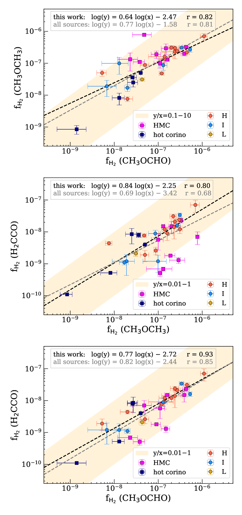
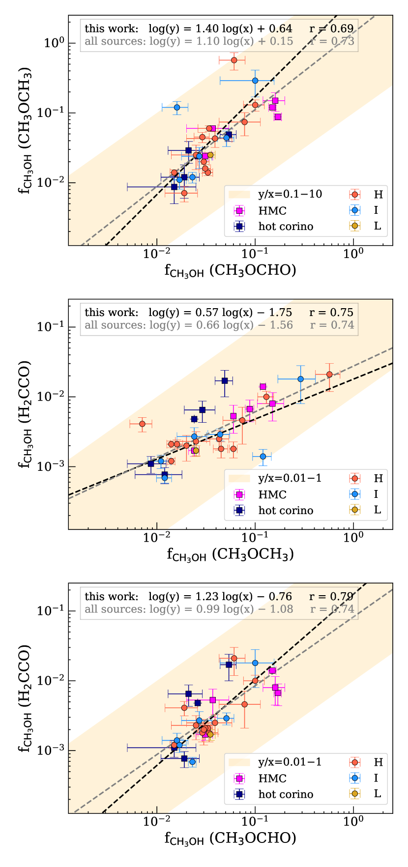
In Figure 3, we compare the CH3OCHO, CH3OCH3, and H2CCO abundances relative to H2 in 19 dense cores. CH3OCHO and CH3OCH3 show a strong abundance correlation (the Pearson correlation coefficient r = 0.82). The abundance correlation between CH3OCH3 and H2CCO is significant (r = 0.80). CH3OCHO and H2CCO show the stronger abundance correlation (r = 0.93) than the other two pairs of molecules. Figure 4 shows the relationships of the abundances of the three molecules relative to CH3OH in 19 dense cores. The abundances of CH3OCHO and CH3OCH3 relative to CH3OH mainly range from 10-2 to 10-1, while the abundance of H2CCO relative to CH3OH mainly ranges from 10-3 to 10-2. The abundances of the three molecules relative to CH3OH in our observations are consistent with those observed in high-mass star-forming regions (Bøgelund et al., 2019; Peng et al., 2022; Chen et al., 2023; López-Gallifa et al., 2024), intermediate-mass star-forming regions (Palau et al., 2011; Fuente et al., 2014; Ospina-Zamudio et al., 2018), low-mass star-forming regions (Taquet et al., 2015; Lefloch et al., 2017; Jørgensen et al., 2018), Galactic center molecular clouds (Requena-Torres et al., 2006; Requena-Torres et al., 2008), and comets (Biver & Bockelée-Morvan, 2019). The correlation coefficients of the abundances relative to CH3OH are 0.69 between CH3OCHO and CH3OCH3, 0.75 between CH3OCH3 and H2CCO, and 0.79 between CH3OCHO and H2CCO, indicating positive correlations. The obvious abundance correlation relative to CH3OH between CH3OCHO and CH3OCH3 was also observed in four different interstellar sources, including 1 HMC, 1 hot corino, and 2 comets (López-Gallifa et al., 2024). From Figure 3 and Figure 4, the relative abundances of CH3OCHO to CH3OCH3 are almost constant equal to 1. Chen et al. (2023) also found a constant relative abundance of 1 between CH3OCHO and CH3OCH3 toward 19 protostars with different luminosities. This ratio is consistent with the observations from low-, intermediate- and high-mass star-forming regions (Jaber et al., 2014; Rivilla et al., 2017; Ospina-Zamudio et al., 2018; Coletta et al., 2020; Peng et al., 2022). In Figure 3 and Figure 4, we also compared our results with the molecular abundances relative to H2 and CH3OH in other HMCs and hot corinos. The abundance correlations relative to H2 and CH3OH in these sources agree with the results in our observations but more dispersed than our samples, which is most likely due to different spatial resolution and spectral setup of these observations. These results suggest that the formation of the three molecules may be closely related, i.e., they may have similar production conditions, or even share a common chemical reaction network.
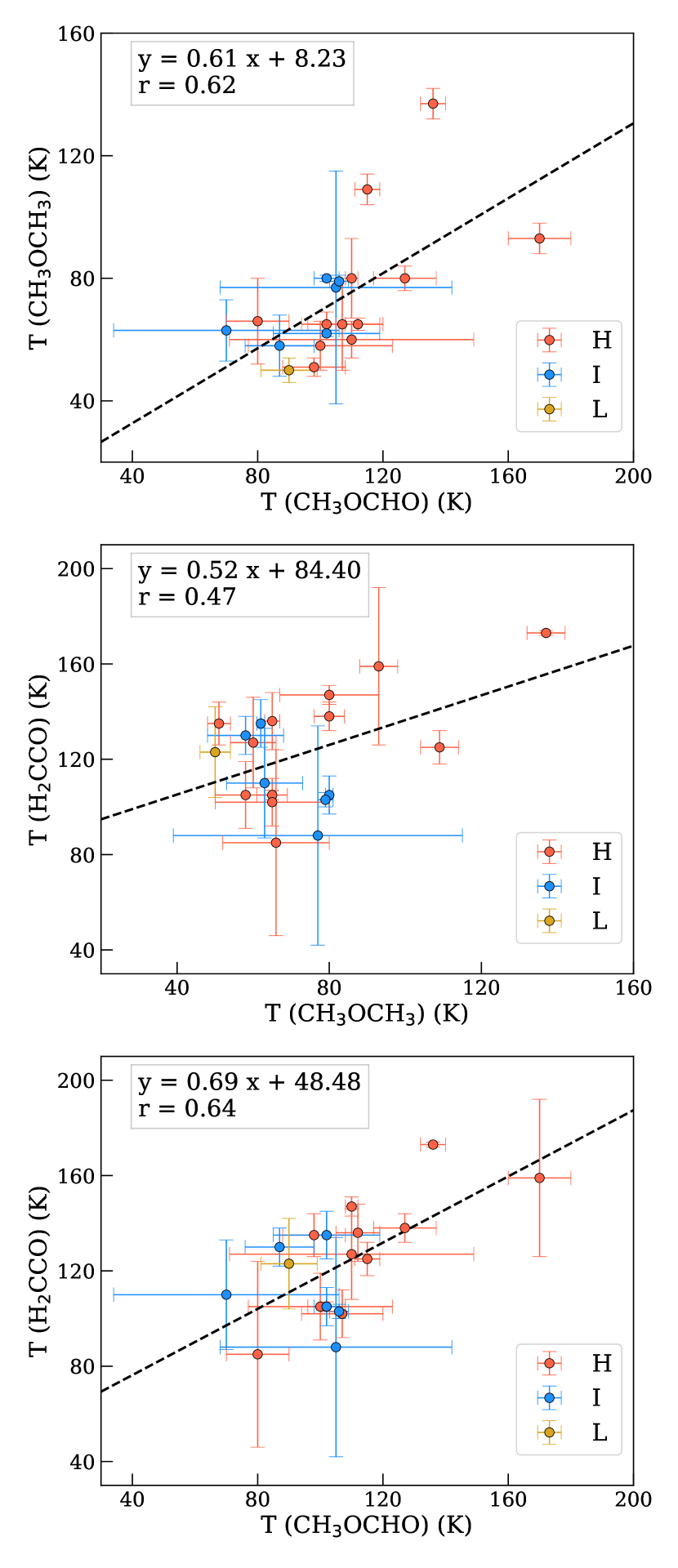
In Figure 5, we compare the rotation temperatures of the three molecules. The temperature correlation coefficient of CH3OCHO and CH3OCH3 is 0.62, CH3OCH3 and H2CCO is 0.47, and CH3OCHO and H2CCO is 0.64. The results indicate that the rotation temperatures have no significant correlations among the three molecules. The results observed by Coletta et al. (2020) toward 13 high-mass star-forming regions also showed a poor temperature correlation (r = 0.45) between CH3OCHO and CH3OCH3, but the overall temperature ranges of the two molecules are similar. In fact, most of the temperatures of the three molecules in our case are in the range of tens of Kelvin, which is probably the reason why there is no apparent trend in temperature.
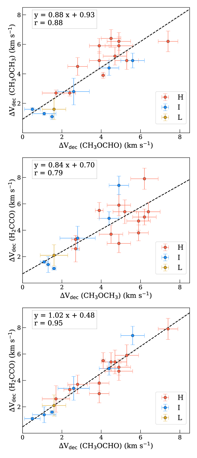
The line width relationships of the three molecules are shown in Figure 6. The CH3OCHO and H2CCO show strong line width correlation (r = 0.95), followed by CH3OCHO and CH3OCH3 (r = 0.88), and by CH3OCH3 and H2CCO (r = 0.79). This agrees with the line width correlation of CH3OCHO and CH3OCH3 observed in 13 high-mass star-forming regions (Coletta et al., 2020). This implies that the three molecules may trace the similar kinematics.444In our case, the line widths of the three molecules are almost entirely contributed by non-thermal motions: Vdec VNT = , where VNT is the line width contributed by non-thermal motions, k is the Boltzmann constant, Tex is the excitation temperature of the molecule, and m is the molecular mass.
In Figures 3, 5, and 6, the H cores are shifted to the upper right relative to the I and L cores, indicating a tendency for the abundances relative to H2, temperatures and line widths of the three molecules to be higher in massive line-rich cores. In Figure 7, we also compare molecular abundances relative to H2 and CH3OH, rotation temperatures and line widths of the cores with and without detected outflows (see Table 1). The abundances relative to H2, temperatures and line widths of the three molecules tend to be higher where outflows are detected. These results confirm that massive cores and cores with outflows may have richer chemistry (Jørgensen et al., 2020; Ceccarelli et al., 2023).
4.3 Implications for Chemistry
The spatial similarities, abundance correlations and line width correlations of CH3OCHO, CH3OCH3, and H2CCO are obvious. We briefly summarize the chemical models of these three molecules below. In gas-phase chemistry, protonated methanol (CH3OH) can react with CH3OH to produce CH3OCH3 as follows (Charnley et al., 1995; Taquet et al., 2016; Jørgensen et al., 2020):
| (8) |
Balucani et al. (2015) proposed that CH3OCH3 could generate CH3OCHO in cold gas environments through the following reactions:
| (9) |
where CH3OCH3 is a precursor to CH3OCHO. In the case of grain-surface chemistry, the CH3OCHO and CH3OCH3 follow the reactions (Garrod & Herbst, 2006; Garrod et al., 2008):
| (10) |
| (11) |
where methoxide (CH3O) is the common precursor of CH3OCHO and CH3OCH3. On the surface of the dust grains, the aldehyde (HCO) can produce H2CCO as follows (Charnley et al., 2001; Charnley & Rodgers, 2005; Krasnokutski et al., 2017):
| (12) |
| (13) |
where HCO is the common precursor of CH3OCHO and H2CCO through Eq. (10) (12). The spatial similarities, abundance correlations, and line width correlations of CH3OCHO, CH3OCH3, and H2CCO, combined with chemical models, suggest that three molecules are chemically related. Taquet et al. (2016) predicted the abundances of CH3OCH3 relative to H2 to be 10-7 and relative to CH3OH to be 10-2 using reaction (8). Our observed abundances of CH3OCH3 relative to H2 and CH3OH are consistent with this prediction. Garrod et al. (2022) showed a chemical network that includes reactions (8), (9), (10), (11), and (13) to predict the abundances of CH3OCHO, CH3OCH3, and H2CCO. The three warm-up timescales of 5 × 10⁴ years (fast), 2 × 10⁵ years (medium), and 1 × 10⁶ years (slow) were employed in their models. At the medium timescale, the predicted abundances relative to H2 are 10-7 for CH3OCHO and CH3OCH3, 10-8 for H2CCO, and relative to CH3OH are 10-2 for CH3OCHO and CH3OCH3, 10-3 for H2CCO. Our observed abundances of the three molecules relative to H2 and CH3OH are consistent with the medium timescale predictions. In conclusion, our observed abundances of the three molecules support both grain-surface and gas-phase chemical pathways for the production of CH3OCHO and CH3OCH3, and grain-surface chemical pathways for the production of H2CCO.
5 Conclusions
We have analyzed the spectra of 11 high-mass star-forming regions obtained by ALMA band 7 observations, and studied the correlations of complex organic molecules CH3OCHO and CH3OCH3 as well as an important precursor of complex organic molecules H2CCO. We summarize the main results in the following:
-
1.
CH3OCHO, CH3OCH3, and H2CCO lines were detected in 19 line-rich cores from 9 out of 11 high-mass star-forming regions. At our higher spatial resolution observations, some of the hot molecular cores found in previous observations are revealed to actually host multiple line-rich cores with different masses.
-
2.
The integrated intensity maps of the 9 high-mass star-forming regions show that the emission peaks of the three molecules are consistent, and the spatial distribution of the molecules is similar. The emissions of the three molecules in the 9 high-mass star-forming regions are primarily distributed around intense continuum emission.
-
3.
The abundances relative to H2 and CH3OH, and line widths of the three molecules show obvious correlations in the 19 dense cores. The abundance correlations of the three molecules relative to H2 and CH3OH in other hot molecular cores and hot corinos agree with the results in our observations. The molecular abundances of CH3OCHO and CH3OCH3 are rather similar, while the molecular abundances of H2CCO are one order of magnitude lower.
-
4.
The abundances relative to H2, temperatures and line widths of the three molecules tend to be higher in the cores with higher mass and with outflows. This confirms that massive cores and cores with outflows may have richer chemistry.
-
5.
The spatial similarities, abundance correlations, and line width correlations of CH3OCHO, CH3OCH3, and H2CCO, combined with chemical models, suggest that three molecules are chemically related. Our results suggest that both grain-surface and gas-phase chemical pathways can be responsible for producing CH3OCHO and CH3OCH3, while H2CCO should be produced by grain-surface chemical pathways.
Acknowledgements
This paper makes use of the following ALMA data: ADS/JAO.ALMA#2017.1.00545.S. ALMA is a partnership of ESO (representing its member states), NSF (USA), and NINS (Japan), together with NRC (Canada), MOST and ASIAA (Taiwan), and KASI (Republic of Korea), in cooperation with the Republic of Chile. The Joint ALMA Observatory is operated by ESO, AUI/NRAO, and NAOJ. This work has been supported by National Key R&D Program of China (No. 2022YFA1603101), and by NSFC through the grants No. 12033005, No. 12073061, No. 12122307, and No. 12103045. S.-L. Qin thanks the Xinjiang Uygur Autonomous Region of China for their support through the Tianchi Program. MYT acknowledges the support by NSFC through grants No.12203011, and Yunnan provincial Department of Science and Technology through grant No.202101BA070001-261. T. Zhang thanks the student’s exchange program of the Collaborative Research Centre 956, funded by the Deutsche Forschungsgemeinschaft (DFG).
Data Availability
The data underlying this article are available in the ALMA archive.
References
- Agúndez et al. (2019) Agúndez M., Marcelino N., Cernicharo J., Roueff E., Tafalla M., 2019, A&A, 625, A147
- Bacmann et al. (2012) Bacmann A., Taquet V., Faure A., Kahane C., Ceccarelli C., 2012, A&A, 541, L12
- Balucani et al. (2015) Balucani N., Ceccarelli C., Taquet V., 2015, MNRAS, 449, L16
- Baug et al. (2020) Baug T., et al., 2020, ApJ, 890, 44
- Belloche et al. (2013) Belloche A., Müller H. S. P., Menten K. M., Schilke P., Comito C., 2013, A&A, 559, A47
- Bergner et al. (2017) Bergner J. B., Öberg K. I., Garrod R. T., Graninger D. M., 2017, ApJ, 841, 120
- Bergner et al. (2019) Bergner J. B., Martín-Doménech R., Öberg K. I., Jørgensen J. K., Artur de la Villarmois E., Brinch C., 2019, ACS Earth and Space Chemistry, 3, 1564
- Bianchi et al. (2019) Bianchi E., et al., 2019, MNRAS, 483, 1850
- Biver & Bockelée-Morvan (2019) Biver N., Bockelée-Morvan D., 2019, ACS Earth and Space Chemistry, 3, 1550
- Bøgelund et al. (2019) Bøgelund E. G., Barr A. G., Taquet V., Ligterink N. F. W., Persson M. V., Hogerheijde M. R., van Dishoeck E. F., 2019, A&A, 628, A2
- Bottinelli et al. (2004) Bottinelli S., et al., 2004, ApJ, 615, 354
- Bottinelli et al. (2007) Bottinelli S., Ceccarelli C., Williams J. P., Lefloch B., 2007, A&A, 463, 601
- Cazaux et al. (2003) Cazaux S., Tielens A. G. G. M., Ceccarelli C., Castets A., Wakelam V., Caux E., Parise B., Teyssier D., 2003, ApJ, 593, L51
- Ceccarelli et al. (2023) Ceccarelli C., et al., 2023, in Inutsuka S., Aikawa Y., Muto T., Tomida K., Tamura M., eds, Astronomical Society of the Pacific Conference Series Vol. 534, Protostars and Planets VII. p. 379
- Cernicharo et al. (2012) Cernicharo J., Marcelino N., Roueff E., Gerin M., Jiménez-Escobar A., Muñoz Caro G. M., 2012, ApJ, 759, L43
- Charnley & Rodgers (2005) Charnley S. B., Rodgers S. D., 2005, in Lis D. C., Blake G. A., Herbst E., eds, Vol. 231, Astrochemistry: Recent Successes and Current Challenges. pp 237–246, doi:10.1017/S174392130600723X
- Charnley et al. (1995) Charnley S. B., Kress M. E., Tielens A. G. G. M., Millar T. J., 1995, ApJ, 448, 232
- Charnley et al. (2001) Charnley S. B., Ehrenfreund P., Kuan Y. J., 2001, Spectrochimica Acta Part A: Molecular Spectroscopy, 57, 685
- Chen et al. (2023) Chen Y., et al., 2023, A&A, 678, A137
- Chen et al. (2024) Chen L., et al., 2024, ApJ, 962, 13
- Coletta et al. (2020) Coletta A., Fontani F., Rivilla V. M., Mininni C., Colzi L., Sánchez-Monge Á., Beltrán M. T., 2020, A&A, 641, A54
- Crockett et al. (2015) Crockett N. R., Bergin E. A., Neill J. L., Favre C., Blake G. A., Herbst E., Anderson D. E., Hassel G. E., 2015, ApJ, 806, 239
- Csengeri et al. (2019) Csengeri T., Belloche A., Bontemps S., Wyrowski F., Menten K. M., Bouscasse L., 2019, A&A, 632, A57
- Duley & Williams (1984) Duley W. W., Williams D. A., 1984, Interstellar chemistry
- Favre et al. (2011) Favre C., Despois D., Brouillet N., Baudry A., Combes F., Guélin M., Wootten A., Wlodarczak G., 2011, A&A, 532, A32
- Fedoseev et al. (2022) Fedoseev G., Qasim D., Chuang K.-J., Ioppolo S., Lamberts T., van Dishoeck E. F., Linnartz H., 2022, ApJ, 924, 110
- Feng et al. (2015) Feng S., Beuther H., Henning T., Semenov D., Palau A., Mills E. A. C., 2015, A&A, 581, A71
- Frau et al. (2010) Frau P., et al., 2010, ApJ, 723, 1665
- Friedel & Snyder (2008) Friedel D. N., Snyder L. E., 2008, ApJ, 672, 962
- Fuente et al. (2014) Fuente A., et al., 2014, A&A, 568, A65
- Garrod & Herbst (2006) Garrod R. T., Herbst E., 2006, A&A, 457, 927
- Garrod et al. (2008) Garrod R. T., Widicus Weaver S. L., Herbst E., 2008, ApJ, 682, 283
- Garrod et al. (2022) Garrod R. T., Jin M., Matis K. A., Jones D., Willis E. R., Herbst E., 2022, ApJS, 259, 1
- Gieser et al. (2021) Gieser C., et al., 2021, A&A, 648, A66
- Hasegawa et al. (1992) Hasegawa T. I., Herbst E., Leung C. M., 1992, ApJS, 82, 167
- Herbst & van Dishoeck (2009) Herbst E., van Dishoeck E. F., 2009, ARA&A, 47, 427
- Hudson & Loeffler (2013) Hudson R. L., Loeffler M. J., 2013, ApJ, 773, 109
- Jaber et al. (2014) Jaber A. A., Ceccarelli C., Kahane C., Caux E., 2014, ApJ, 791, 29
- Jørgensen et al. (2018) Jørgensen J. K., et al., 2018, A&A, 620, A170
- Jørgensen et al. (2020) Jørgensen J. K., Belloche A., Garrod R. T., 2020, ARA&A, 58, 727
- Kauffmann et al. (2008) Kauffmann J., Bertoldi F., Bourke T. L., Evans N. J. I., Lee C. W., 2008, A&A, 487, 993
- Krasnokutski et al. (2017) Krasnokutski S. A., et al., 2017, ApJ, 847, 89
- Lefloch et al. (2017) Lefloch B., Ceccarelli C., Codella C., Favre C., Podio L., Vastel C., Viti S., Bachiller R., 2017, MNRAS, 469, L73
- Lis et al. (1991) Lis D. C., Carlstrom J. E., Keene J., 1991, ApJ, 380, 429
- Liu et al. (2016) Liu T., et al., 2016, ApJ, 829, 59
- Liu et al. (2020) Liu T., et al., 2020, MNRAS, 496, 2790
- Liu et al. (2022) Liu H.-L., et al., 2022, MNRAS, 511, 501
- López-Gallifa et al. (2024) López-Gallifa Á., et al., 2024, MNRAS, 529, 3244
- Maity et al. (2014) Maity S., Kaiser R. I., Jones B. M., 2014, ApJ, 789, 36
- Maret et al. (2004) Maret S., et al., 2004, A&A, 416, 577
- McMullin et al. (2007) McMullin J. P., Waters B., Schiebel D., Young W., Golap K., 2007, in Shaw R. A., Hill F., Bell D. J., eds, Astronomical Society of the Pacific Conference Series Vol. 376, Astronomical Data Analysis Software and Systems XVI. p. 127
- Möller et al. (2013) Möller T., Bernst I., Panoglou D., Muders D., Ossenkopf V., Röllig M., Schilke P., 2013, A&A, 549, A21
- Möller et al. (2017) Möller T., Endres C., Schilke P., 2017, A&A, 598, A7
- Müller et al. (2001) Müller H. S. P., Thorwirth S., Roth D. A., Winnewisser G., 2001, A&A, 370, L49
- Müller et al. (2005) Müller H. S. P., Schlöder F., Stutzki J., Winnewisser G., 2005, Journal of Molecular Structure, 742, 215
- Nummelin et al. (2000) Nummelin A., Bergman P., Hjalmarson Å., Friberg P., Irvine W. M., Millar T. J., Ohishi M., Saito S., 2000, ApJS, 128, 213
- Ospina-Zamudio et al. (2018) Ospina-Zamudio J., Lefloch B., Ceccarelli C., Kahane C., Favre C., López-Sepulcre A., Montarges M., 2018, A&A, 618, A145
- Ossenkopf & Henning (1994) Ossenkopf V., Henning T., 1994, A&A, 291, 943
- Palau et al. (2011) Palau A., et al., 2011, ApJ, 743, L32
- Peng et al. (2022) Peng Y., et al., 2022, MNRAS, 512, 4419
- Pickett et al. (1998) Pickett H. M., Poynter R. L., Cohen E. A., Delitsky M. L., Pearson J. C., Müller H. S. P., 1998, J. Quant. Spectrosc. Radiative Transfer, 60, 883
- Qin et al. (2010) Qin S.-L., Wu Y., Huang M., Zhao G., Li D., Wang J.-J., Chen S., 2010, ApJ, 711, 399
- Qin et al. (2015) Qin S.-L., Schilke P., Wu J., Wu Y., Liu T., Liu Y., Sánchez-Monge Á., 2015, ApJ, 803, 39
- Qin et al. (2022) Qin S.-L., et al., 2022, MNRAS, 511, 3463
- Requena-Torres et al. (2006) Requena-Torres M. A., Martín-Pintado J., Rodríguez-Franco A., Martín S., Rodríguez-Fernández N. J., de Vicente P., 2006, A&A, 455, 971
- Requena-Torres et al. (2008) Requena-Torres M. A., Martín-Pintado J., Martín S., Morris M. R., 2008, ApJ, 672, 352
- Rivilla et al. (2017) Rivilla V. M., Beltrán M. T., Cesaroni R., Fontani F., Codella C., Zhang Q., 2017, A&A, 598, A59
- Ruaud et al. (2015) Ruaud M., Loison J. C., Hickson K. M., Gratier P., Hersant F., Wakelam V., 2015, MNRAS, 447, 4004
- Ruffle & Herbst (2000) Ruffle D. P., Herbst E., 2000, MNRAS, 319, 837
- Ruiterkamp et al. (2007) Ruiterkamp R., Charnley S. B., Butner H. M., Huang H. C., Rodgers S. D., Kuan Y. J., Ehrenfreund P., 2007, Ap&SS, 310, 181
- Sánchez-Monge et al. (2010) Sánchez-Monge Á., Palau A., Estalella R., Kurtz S., Zhang Q., Di Francesco J., Shepherd D., 2010, ApJ, 721, L107
- Taquet et al. (2015) Taquet V., López-Sepulcre A., Ceccarelli C., Neri R., Kahane C., Charnley S. B., 2015, ApJ, 804, 81
- Taquet et al. (2016) Taquet V., Wirström E. S., Charnley S. B., 2016, ApJ, 821, 46
- Vasyunin & Herbst (2013) Vasyunin A. I., Herbst E., 2013, ApJ, 769, 34
- Xu et al. (2024) Xu F., et al., 2024, ApJS, 270, 9
- Yan et al. (2019) Yan Y. T., et al., 2019, ApJ, 877, 154
- Zhang et al. (2023) Zhang C., et al., 2023, MNRAS, 520, 3245
- van ’t Hoff et al. (2020) van ’t Hoff M. L. R., Bergin E. A., Jørgensen J. K., Blake G. A., 2020, ApJ, 897, L38
Appendix A Spectra of line-rich cores
The spectra and optical depths of the three molecules detected in the 19 line-rich cores are shown in Figure 1 and Figure 8.
Appendix B Molecular Transitions
The rotational transitions of the three molecules detected in 19 dense cores are shown in Table 4. The molecular parameters are taken from the JPL catalogue for CH3OCHO lines and the CDMS catalogue for CH3OCH3 and H2CCO lines. Due to internal rotation, the CH3OCHO rotational levels split into two substates A and E, while the CH3OCH3 rotational levels split into four substates AA, EE, EA, and AE.
| Frequency | Transition | S2 | Eup |
|---|---|---|---|
| (MHz) | (D2) | (K) | |
| CH3OCHO (v=0) | |||
| 342342.185 | 30(2,28)29(3,27) E | 10.00 | 269.50 |
| 342350.119 | 30(2,28)29(3,27) A | 10.00 | 269.49 |
| 342351.420 | 30(3,28)29(3,27) E | 78.04 | 269.50 |
| 342358.225 | 30(2,28)29(2,27) E | 78.03 | 269.50 |
| 342359.508 | 30(3,28)29(3,27) A | 78.03 | 269.49 |
| 342366.296 | 30(2,28)29(2,27) A | 78.03 | 269.49 |
| 342367.680 | 30(3,28)29(2,27) E | 10.00 | 269.50 |
| 342375.658 | 30(3,28)29(2,27) A | 10.00 | 269.49 |
| 342506.986 | 11(8,4)10(7,4) E | 3.46 | 81.40 |
| 342525.299 | 11(8,3)10(7,3) E | 3.46 | 81.42 |
| 342572.422 | 11(8,4)10(7,3) A | 3.46 | 81.41 |
| 342572.422 | 11(8,3)10(7,4) A | 3.46 | 81.41 |
| 342678.725 | 27(13,15)27(12,16) E | 5.56 | 335.27 |
| 342680.167 | 27(13,14)27(12,15) E | 5.56 | 335.28 |
| 342692.876 | 27(13,14)27(12,15) A | 5.56 | 335.28 |
| 342692.888 | 27(13,15)27(12,16) A | 5.56 | 335.28 |
| 343096.392 | 17(5,12)16(4,13) E | 1.87 | 107.82 |
| 343136.353 | 26(13,13)26(12,14) E | 5.23 | 319.30 |
| 343136.356 | 26(13,14)26(12,15) E | 5.23 | 319.29 |
| 343147.898 | 31(1,30)30(2,29) E | 11.85 | 273.44 |
| 343148.047 | 31(2,30)30(2,29) E | 81.50 | 273.44 |
| 343148.169 | 31(1,30)30(1,29) E | 81.50 | 273.44 |
| 343148.318 | 31(2,30)30(1,29) E | 11.85 | 273.44 |
| 343149.303 | 17(5,12)16(4,13) A | 1.87 | 107.81 |
| 343152.958 | 31(1,30)30(2,29) A | 11.89 | 273.43 |
| 343153.106 | 31(2,30)30(2,29) A | 81.46 | 273.43 |
| 343153.227 | 31(1,30)30(1,29) A | 81.46 | 273.43 |
| 343153.376 | 31(2,30)30(1,29) A | 11.89 | 273.43 |
| 343153.762 | 26(13,13)26(12,14) A | 5.23 | 319.30 |
| 343153.770 | 26(13,14)26(12,15) A | 5.23 | 319.30 |
| 343435.260 | 28(4,24)27(4,23) E | 71.57 | 257.08 |
| 343443.944 | 28(4,24)27(4,23) A | 71.58 | 257.08 |
| 343539.815 | 25(13,12)25(12,13) E | 4.90 | 303.92 |
| 343541.355 | 25(13,13)25(12,14) E | 4.90 | 303.91 |
| 343561.850 | 25(13,12)25(12,13) A | 4.90 | 303.92 |
| 343561.883 | 25(13,13)25(12,14) A | 4.90 | 303.92 |
| 343731.783 | 27(7,20)26(7,19) E | 67.17 | 258.47 |
| 343758.010 | 27(7,20)26(7,19) A | 67.19 | 258.48 |
| 343798.647 | 28(23,5)27(23,4) A | 24.44 | 589.86 |
| 343798.647 | 28(23,6)27(23,5) A | 24.44 | 589.86 |
| 343814.031 | 28(23,5)27(23,4) E | 24.44 | 589.86 |
| 343826.593 | 28(23,6)27(23,5) E | 24.44 | 589.85 |
| 343835.114 | 28(22,7)27(22,6) A | 28.73 | 560.10 |
| 343835.114 | 28(22,6)27(22,5) A | 28.73 | 560.10 |
| 343854.153 | 28(22,6)27(22,5) E | 28.74 | 560.10 |
| 343862.096 | 28(22,7)27(22,6) E | 28.73 | 560.09 |
| 343887.467 | 28(21,8)27(21,7) A | 32.84 | 531.66 |
| 343887.483 | 28(21,7)27(21,6) A | 32.84 | 531.66 |
| 343895.152 | 24(13,11)24(12,12) E | 4.57 | 289.13 |
| 343898.142 | 24(13,12)24(12,13) E | 4.57 | 289.13 |
| 343909.244 | 28(21,7)27(21,6) E | 32.83 | 531.65 |
| 343912.685 | 28(21,8)27(21,7) E | 32.84 | 531.65 |
| 343921.695 | 24(13,11)24(12,12) A | 4.57 | 289.14 |
| 343921.695 | 24(13,12)24(12,13) A | 4.57 | 289.14 |
| 343958.362 | 28(20,9)27(20,8) A | 36.75 | 504.53 |
| 343958.362 | 28(20,8)27(20,7) A | 36.75 | 504.53 |
| 343981.148 | 28(20,9)27(20,8) E | 36.74 | 504.52 |
| 343982.450 | 28(20,8)27(20,7) E | 36.74 | 504.52 |
| 344029.259 | 32(0,32)31(1,31) E | 10.53 | 276.10 |
| 344029.260 | 32(1,32)31(1,31) E | 88.18 | 276.10 |
| Frequency | Transition | S2 | Eup |
|---|---|---|---|
| (MHz) | (D2) | (K) | |
| CH3OCHO (v=0) | |||
| 344029.261 | 32(0,32)31(0,31) E | 88.18 | 276.10 |
| 344029.262 | 32(1,32)31(0,31) E | 10.53 | 276.10 |
| 344029.645 | 32(0,32)31(1,31) A | 13.73 | 276.08 |
| 344029.645 | 32(1,32)31(1,31) A | 84.98 | 276.08 |
| 344029.646 | 32(0,32)31(0,31) A | 84.98 | 276.08 |
| 344029.647 | 32(1,32)31(0,31) A | 13.73 | 276.08 |
| 344051.371 | 28(19,10)27(19,9) A | 40.46 | 478.72 |
| 344051.371 | 28(19,9)27(19,8) A | 40.46 | 478.72 |
| 344071.196 | 28(19,9)27(19,8) E | 40.45 | 478.72 |
| 344076.934 | 28(19,10)27(19,9) E | 40.45 | 478.72 |
| 344170.930 | 28(18,10)27(18,9) A | 43.97 | 454.24 |
| 344170.930 | 28(18,11)27(18,10) A | 43.97 | 454.24 |
| 344187.246 | 28(18,10)27(18,9) E | 43.98 | 454.24 |
| 344197.339 | 28(18,11)27(18,10) E | 43.97 | 454.24 |
| 344206.436 | 23(13,10)23(12,11) E | 4.23 | 274.95 |
| 344210.812 | 23(13,11)23(12,12) E | 4.23 | 274.94 |
| 344237.391 | 23(13,10)23(12,11) A | 4.23 | 274.95 |
| 344237.414 | 23(13,11)23(12,12) A | 4.23 | 274.95 |
| 344322.992 | 28(17,12)27(17,11) A | 47.30 | 431.09 |
| 344322.992 | 28(17,11)27(17,10) A | 47.30 | 431.09 |
| 344335.357 | 28(17,11)27(17,10) E | 47.30 | 431.08 |
| 344349.515 | 28(17,12)27(17,11) E | 47.30 | 431.08 |
| 344477.576 | 22(13,9)22(12,10) E | 3.89 | 261.36 |
| 344483.461 | 22(13,10)22(12,11) E | 3.89 | 261.35 |
| 344512.739 | 22(13,9)22(12,10) A | 3.89 | 261.37 |
| 344512.747 | 22(13,10)22(12,11) A | 3.89 | 261.37 |
| 344515.454 | 28(16,13)27(16,12) A | 50.43 | 409.27 |
| 344515.454 | 28(16,12)27(16,11) A | 50.43 | 409.27 |
| 344523.525 | 28(16,12)27(16,11) E | 50.43 | 409.26 |
| 344541.314 | 28(16,13)27(16,12) E | 50.43 | 409.26 |
| 344712.139 | 21(13,8)21(12,9) E | 3.55 | 248.37 |
| 344719.465 | 21(13,9)21(12,10) E | 3.55 | 248.36 |
| 344751.514 | 21(13,9)21(12,10) A | 3.55 | 248.37 |
| 344751.524 | 21(13,8)21(12,9) A | 3.55 | 248.37 |
| 344759.096 | 28(15,14)27(15,13) A | 53.37 | 388.78 |
| 344759.096 | 28(15,13)27(15,12) A | 53.37 | 388.78 |
| 344762.590 | 28(15,13)27(15,12) E | 53.37 | 388.78 |
| 344783.597 | 28(15,14)27(15,13) E | 53.38 | 388.78 |
| 344913.684 | 20(13,7)20(12,8) E | 3.20 | 235.98 |
| 344922.458 | 20(13,8)20(12,9) E | 3.20 | 235.97 |
| 344957.101 | 20(13,8)20(12,9) A | 3.20 | 235.98 |
| 344957.127 | 20(13,7)20(12,8) A | 3.20 | 235.98 |
| 344982.605 | 47(6,41)47(5,42) E | 2.31 | 104.43 |
| 345067.795 | 28(14,14)27(14,13) E | 56.12 | 369.64 |
| 345069.059 | 28(14,15)27(14,14) A | 56.12 | 369.64 |
| 345069.059 | 28(14,14)27(14,13) A | 56.12 | 369.64 |
| 345073.057 | 16(6,11)15(5,10) A | 2.71 | 104.42 |
| 345085.394 | 19(13,6)19(12,7) E | 2.85 | 224.18 |
| 345091.465 | 28(14,15)27(14,14) E | 56.12 | 369.64 |
| 345095.559 | 19(13,7)19(12,8) E | 2.85 | 224.17 |
| 345132.629 | 19(13,6)19(12,7) A | 2.85 | 224.18 |
| 345132.655 | 19(13,7)19(12,8) A | 2.85 | 224.18 |
| 345230.296 | 18(13,5)18(12,6) E | 2.48 | 212.97 |
| 345241.935 | 18(13,6)18(12,7) E | 2.48 | 212.96 |
| 345281.320 | 18(13,6)18(12,7) A | 2.48 | 212.97 |
| 345281.320 | 18(13,5)18(12,6) A | 2.48 | 212.97 |
| 345351.333 | 17(13,4)17(12,5) E | 2.11 | 202.36 |
| 345364.235 | 17(13,5)17(12,6) E | 2.11 | 202.34 |
| 345385.268 | 16(6,10)15(5,10) E | 0.40 | 104.45 |
| 345405.869 | 17(13,5)17(12,6) A | 2.11 | 202.36 |
| Frequency | Transition | S2 | Eup |
|---|---|---|---|
| (MHz) | (D2) | (K) | |
| CH3OCHO (v=0) | |||
| 345405.869 | 17(13,4)17(12,5) A | 2.11 | 202.36 |
| 345451.103 | 16(13,3)16(12,4) E | 1.73 | 192.34 |
| 345461.011 | 28(13,15)27(13,14) E | 58.68 | 351.85 |
| 345465.345 | 16(13,4)16(12,5) E | 1.73 | 192.32 |
| 345466.962 | 28(13,16)27(13,15) A | 58.67 | 351.86 |
| 345466.962 | 28(13,15)27(13,14) A | 58.67 | 351.86 |
| 345486.602 | 28(13,16)27(13,15) E | 58.68 | 351.85 |
| 345509.021 | 16(13,4)16(12,5) A | 1.73 | 192.34 |
| 345509.021 | 16(13,3)16(12,4) A | 1.73 | 192.34 |
| 345532.134 | 15(13,2)15(12,3) E | 1.33 | 182.91 |
| 345547.616 | 15(13,3)15(12,4) E | 1.33 | 182.89 |
| 345593.318 | 15(13,3)15(12,4) A | 1.33 | 182.91 |
| 345593.318 | 15(13,2)15(12,3) A | 1.33 | 182.91 |
| 345596.828 | 14(13,1)14(12,2) E | 0.91 | 174.07 |
| 345613.535 | 14(13,2)14(12,3) E | 0.91 | 174.06 |
| 345647.338 | 13(13,0)13(12,1) E | 0.47 | 165.83 |
| 345650.835 | 9(9,1)8(8,1) E | 3.90 | 80.31 |
| 345661.070 | 14(13,1)14(12,2) A | 0.91 | 174.07 |
| 345661.070 | 14(13,2)14(12,3) A | 0.91 | 174.07 |
| 345662.771 | 9(9,0)8(8,0) E | 3.90 | 80.33 |
| 345665.188 | 13(13,1)13(12,2) E | 0.47 | 165.81 |
| 345714.339 | 13(13,0)13(12,1) A | 0.47 | 165.83 |
| 345714.339 | 13(13,1)13(12,2) A | 0.47 | 165.83 |
| 345718.662 | 9(9,1)8(8,0) A | 3.90 | 80.32 |
| 345718.662 | 9(9,0)8(8,1) A | 3.90 | 80.32 |
| 345974.664 | 28(12,16)27(12,15) E | 61.04 | 335.43 |
| 345985.381 | 28(12,17)27(12,16) A | 61.05 | 335.43 |
| 345985.381 | 28(12,16)27(12,15) A | 61.05 | 335.43 |
| 346001.616 | 28(12,17)27(12,16) E | 61.04 | 335.43 |
| CH3OCH3 (v=0) | |||
| 342607.898 | 19(0,19)18(1,18) EA | 110.05 | 167.14 |
| 342607.898 | 19(0,19)18(1,18) AE | 165.08 | 167.14 |
| 342607.971 | 19(0,19)18(1,18) EE | 440.24 | 167.14 |
| 342608.044 | 19(0,19)18(1,18) AA | 275.16 | 167.14 |
| 343753.320 | 17(2,16)16(1,15) EA | 29.01 | 143.70 |
| 343753.320 | 17(2,16)16(1,15) AE | 58.02 | 143.70 |
| 343754.216 | 17(2,16)16(1,15) EE | 232.07 | 143.70 |
| 343755.112 | 17(2,16)16(1,15) AA | 87.02 | 143.70 |
| 344357.816 | 19(1,19)18(0,18) EA | 55.06 | 167.18 |
| 344357.816 | 19(1,19)18(0,18) AE | 110.12 | 167.18 |
| 344357.929 | 19(1,19)18(0,18) EE | 440.51 | 167.18 |
| 344358.041 | 19(1,19)18(0,18) AA | 165.18 | 167.18 |
| 344512.176 | 11(3,9)10(2,8) EA | 25.13 | 72.78 |
| 344512.219 | 11(3,9)10(2,8) AE | 12.57 | 72.78 |
| 344515.385 | 11(3,9)10(2,8) EE | 100.53 | 72.78 |
| 344518.572 | 11(3,9)10(2,8) AA | 37.70 | 72.78 |
| H2CCO (v=0) | |||
| 343088.615 | 17(5,13)16(5,12) | 93.93 | 473.85 |
| 343088.615 | 17(5,12)16(5,11) | 93.93 | 473.85 |
| 343172.572 | 17(0,17)16(0,16) | 34.28 | 148.30 |
| 343250.411 | 17(4,14)16(4,13) | 32.38 | 356.84 |
| 343250.411 | 17(4,13)16(4,12) | 32.38 | 356.84 |
| 343376.133 | 17(2,16)16(2,15) | 33.81 | 200.53 |
| 343384.676 | 17(3,15)16(3,14) | 99.64 | 265.71 |
| 343387.579 | 17(3,14)16(3,13) | 99.64 | 265.71 |
| 343693.935 | 17(2,15)16(2,14) | 33.81 | 200.61 |
-
Notes. The rest frequencies are listed and the transitions are in the form of J(Ka,Kc)J′(Ka′,Kc′). The S2 is the product of the line strength and the square of the relevant dipole moment. The Eup is the upper level energy of each transition.
Appendix C Molecular Emission
We compare the molecular emissions of CH3OCHO with different energy level transitions. The integrated intensity maps of CH3OCHO at 342572 MHz (Eu = 81 K) and at 342359 MHz (Eu = 269 K) in 9 high-mass star-forming regions are shown in Figure 9. In the 9 high-mass star-forming regions, there is no difference in the spatial emission between the different energy level transitions of CH3OCHO.