Correlation Clustering Algorithm for Dynamic Complete Signed Graphs: An Index-based Approach

Clustering is one of the most studied problems in machine learning with various applications in analyzing and visualizing large datasets. There are various models and technique to obtain a partition of elements, such that elements belonging to different partitions are dissimilar to each other and the elements in the same partition are very similar to each other.

The problem of correlation clustering, introduced in [1], is known to be an NP-hard problem for the disagree minimization. Therefore, several different approximation solutions based on its IP formulation exist in the literature. Recently, the idea of a 2-approximation algorithm in [1] is extended in [4] for constructing a $\mathcal{O}\left(1\right)$-approximation algorithm. The experiments in [4] show acceptable performance for this algorithm in practice, although its theoretical guarantee can be too high, e.g. $1\,442$ for $\beta=\lambda=\frac{1}{36}$. In [3], this algorithm is extended to an online setting where just vertex additions are allowed, and whenever a new vertex is added, it reveals all its positively signed edges. Shakiba in [12] studied the effect of vertex addition/removal and edge sign flipping in the underlying graph to the final clustering result, in order to make the algorithm suitable for dynamic graphs. However, one bottleneck in this way is computing the values of NonAgreement among the edges and identifying the $\varepsilon$-lightness of vertices. The current paper proposes a novel indexing scheme to remedy this and make the algorithm efficient, not just in terms of dynamic graphs, but for even dynamic hyper-parameter $\varepsilon$. Our proposed method, in comparison with the online method of [3] is that we allow a full dynamic setting, i.e. vertex addition/removal and edge’s sign flipping. It is known that any online algorithm for the correlation clustering problem has at least $\Omega(n)$-approximation ratio [10]. Note that the underlying algorithm used in the current paper is consistent, as is shown via experimental results [3].

The rest of the paper is organized as follows: In Section 1.1, we highlight our contributions. This is followed by a reminding some basic algorithms and results in Section 2. Then, we introduce the novel indexing structure in Section 3.1 and show how it can be employed to enhance the running-time of the approximate correlation clustering algorithm. Then, we show how to maintain the proposed indices in a full dynamic settings in Section 3.2. In Section 4, we give an extensive experiments which accompanies the theoretical results and show the effectiveness of the proposed indexing structure. Finally, a conclusion is drawn.

Let $G=(V,E)$ be a complete undirected signed graph with $\left|V\right|=n$ vertices. The set of edges $E$ is naturally partitioned into positive and negative signed edges, $E^{+}$ and $E^{-}$, respectively. Then, we use $m$ to denote $\left|E^{+}\right|$. The correlation clustering problem is defined as

where $\mathcal{C}=\left\{C_{1},\ldots,C_{\ell}\right\}$ is a clustering. Note that this is the min-disagree variant of the problem.

The constant factor approximation algorithm of [4] is based on two main quantities: (1) $\varepsilon$-agreement of a positively signed edge $\left\{u,v\right\}$, i.e. $u$ and $v$ are in $\varepsilon$-agreement if and only if $\textsc{NonAgreement}_{G}\left(u,v\right)=\frac{\left|N_{G}(u)\Delta N_{G}(v)\right|}{\max\left\{\left|N_{G}(u)\right|,\left|N_{G}(v)\right|\right\}}<\varepsilon$, and (2) $\varepsilon$-lightness, where a vertex $u$ is said to be $\varepsilon$-light if $\frac{\textsc{AgreeCnt}_{G^{+}}(u)}{\left|N_{G^{+}}(u)\right|}<\varepsilon$ where $\textsc{AgreeCnt}_{G^{+}}(u)=\left|\left\{w\in V|u\text{ and }v\text{ are in }\varepsilon\text{-agreement}\right\}\right|$. Note that a vertex which is not $\varepsilon$-light is called $\varepsilon$-heavy. This is a $2+\frac{4}{\varepsilon}+\frac{1}{\varepsilon^{2}}$-approximation algorithm, as is shown in [3]. This algorithm is described in Algorithm 1, which we will refer to the CC algorithm, for short.

Shakiba in [12] studied theoretical foundation of the CC algorithm in a full dynamic setting. The following result is a summary of Table 1, Corollary 1, and Theorem 4 in [12].

The arboricity of the graph $G$ is the minimum number of edge-disjoint spanning forests into which $G$ can be decomposed. The following lemma for arboricity is useful in bounding the number of operations.

In this section, we describe our novel indexing structure. This structure allows dynamic queries of the correlation clustering with varying values of $\varepsilon$ for dynamic graphs. The proposed algorithm which uses the indexing structure would be called ICC, or indexed-based correlation clustering.

To evaluate the proposed method, we used 7 graphs which are formed by user-user interactions. These datasets are described in Table 1 and are accessible through the SNAP [8]. The smallest dataset consists of 22 470 nodes with 171 002 edges and the largest one consists of 317 080 nodes with 1 049 866 edges. In all these graphs, we consider the existing edges as positively signed and non-existing edges as negatively signed.

The distribution of the NonAgreements for each dataset is illustrated in Figures 2(a) to 8(a). The distribution of NonAgreements of the edges in almost all the datasets obeys the normal distribution, except small imperfections in Arxiv ASTRO-PH (Figure 2(a)), Arxiv COND-MAT (Figure 4(a)), and DBLP (Figure 8(a)). Moreover, more detailed statistics on these distributions are given in Tables 2. One single observation is that the most frequent value of the NonAgreement in all the sample datasets is $1$. Why is that? Without loss of generality, assume that $\deg_{G}(u)\geq\deg_{G}(v)$. Then, $\left|N_{G}(v)\right|=2\left|N_{G}(u)\cap N_{G}(v)\right|$. By the assumption $\left|N_{G}(u)\right|\geq 2\left|N_{G}(u)\cap N_{G}(v)\right|$, i.e. the intersection of the neighborhood of vertices $u$ and $v$ consists of at most half of the neighborhood of $u$. Also, exactly half of the neighborhood of $v$ falls at the intersection of the neighborhood of $u$ and $v$. Intuitively, the vertex $u$ has clustering preference with extra vertices at least the number of vertices which both $u$ and $v$ have clustering preference. Similarly, the vertex $v$ has clustering preference with exactly half extra vertices which both $u$ and $v$ have clustering preference.

For each dataset, we have used a different set of $\varepsilon$-Schedules, depending on the distribution of their NonAgreements. More precisely: (1) we have sorted the values of non-agreements in each dataset in a non-decreasing order, with repetitions. (2) Then, we have selected $21$ distinct values equally spaces of these values. (3) The $\varepsilon$-Schedule was set to the selected values in the second step, which appended the value of $0$ at the beginning and the value of $1.99$ to the end if either does not exists. Totally, the number of $\varepsilon$-Schedule for each dataset is either $21$, $22$ or $23$.

An interesting observation is the number of clusters for $\varepsilon\approx 1^{-}$ in Figures 2(b) to 8(b). Note that we use $1^{-}$ to denote the interval $[1-\epsilon,1]$ for some non-zero constant $\epsilon>0$. When $\varepsilon\approx 1$ but less than $1$, the number of clusters is minimum. As it gets closer to $1$, the number of clusters increases with a much greater descent than the decrease in the number of clusters as it gets close to $1$ from $0$.

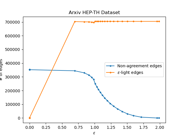
As in Corollary 1, by increasing the $\varepsilon$, the number of vertices in $\varepsilon$-agreement is a non-decreasing function, which is confirmed by the plots in Figures 2(a) to 8(a) as the number of vertices in $\varepsilon$-non-agreement is given by a non-increasing function. By closer visual inspection of these figures, we can see that the shape of the plot for the number of $\varepsilon$-non-agreement vertices in all these graphs is almost the same, with inflection point around the value of $\varepsilon\approx 1$. This is due to the intrinsic nature of the $\textsc{NonAgreement}_{G}\left(u,v\right)$.

Similarly, the non-monotonicity result stated in Corollary 1 is observed in the same figures for the number of $\varepsilon$-light vertices. By a visual inspection, the trend of the number of $\varepsilon$-light vertices for almost all datasets, except for the Arxiv HEP-TH (Figure 5(a)) and the EU-Email (Figure 7(a)), is the same: the number of $\varepsilon$-light vertices increases as $\varepsilon$ increases up to some point (first interval), then decreases slightly (second interval), and finally increases and would be asymptotically equal to the number of vertices in the graphs (last interval). For Arxiv HEP-TH and EU-Email, we have the same trend, however, the second interval is very small.

All the algorithms for the naive and the proposed index-based correlation clustering algorithms are implemented in C++¹¹1https://github.com/alishakiba/Correlation-Clustering-Algorithm-for-Dynamic-Complete-Signed-Graphs-An-Index-based-Approach without any parallelization and the experiments are done using an Ubuntu 22.04.1 TLS with an Intel Core i7-10510U CPU @ 1.80GHz with 12 GB of RAM. The time for running the naive correlation clustering algorithm (Algorithm 1), denoted here as CC, as well as the time for the index-based correlation clustering algorithm denoted as ICC, is given in Figures 2(d) to 8(d)). Note that the time reported for the ICC in these figures does not include the required time for constructing the $\mathbb{NAO}$s, as they are constructed once and used throughout the $\varepsilon$-Schedule. The running-time to read the graph as well as constructing the $\mathbb{NAO}$s is reported in Table 3 in milliseconds. The CC and ICC algorithms are the same, except that in CC, the non-agreement values of the edges and the $\varepsilon$-lightness of the vertices are computed for each given value of $\varepsilon$, however, in ICC these are computed and stored in the proposed $\mathbb{NAO}$s structure once and used for clustering with respect to different values of $\varepsilon$. As it can be observed in Figures 2(d) to 8(d), the running time for the ICC, excluding the time to construct the $\mathbb{NAO}$s for once, is largely smaller than the one for CC. On average, our approach for the described $\varepsilon$-Schedule lead to $\%25$ decrease in clustering time. This enhancement comes at the cost of pre-computing the $\mathbb{NAO}$s, which costs on average $\%34$ of the time for a single run of CC, which is quite small and makes the ICC efficient in cases where one requires to have multiple clustering for various values of $\varepsilon$.

In this paper, we proposed a novel indexing structure to decrease the overall running-time of an approximation algorithm for the correlation clustering problem. This structure can be constructed in $\mathcal{O}\left(m\times\alpha(G)\right)$ time with $\mathcal{O}\left(m\right)$ memory. Then, we can output a correlation clustering for any value of $\varepsilon$ in $\mathcal{O}\left(m+n\right)$, compared with $\mathcal{O}\left(m\times\left(2+\alpha(G)\right)+n\right)$ time complexity of the ordinary correlation clustering algorithm. Moreover, the proposed index can be efficiently maintained during updates to the underlying graph, including edge sign flip, vertex addition and vertex deletion. The theoretical results are accompanied with practical results in the experiments using seven real world graphs. The experimental results show about %34 decrease in the running-time of queries.

A future research direction would be studying this algorithm in parallel frameworks such as Map-Reduce and make it scalable to very Big graphs. Another research direction would be enhancing the approximation guarantee of the algorithm, or devising more efficient algorithms in terms of approximation ratio.

References

- [1] Nikhil Bansal, Avrim Blum, and Shuchi Chawla. Correlation clustering. Machine learning, 56(1):89–113, 2004.
- [2] Norishige Chiba and Takao Nishizeki. Arboricity and subgraph listing algorithms. SIAM Journal on computing, 14(1):210–223, 1985.
- [3] Vincent Cohen-Addad, Silvio Lattanzi, Andreas Maggiori, and Nikos Parotsidis. Online and consistent correlation clustering. In Kamalika Chaudhuri, Stefanie Jegelka, Le Song, Csaba Szepesvari, Gang Niu, and Sivan Sabato, editors, Proceedings of the 39th International Conference on Machine Learning, volume 162 of Proceedings of Machine Learning Research, pages 4157–4179. PMLR, 17–23 Jul 2022.
- [4] Vincent Cohen-Addad, Silvio Lattanzi, Slobodan Mitrović, Ashkan Norouzi-Fard, Nikos Parotsidis, and Jakub Tarnawski. Correlation clustering in constant many parallel rounds. In International Conference on Machine Learning (ICML), pages 2069–2078. PMLR, 2021.
- [5] Thomas H Cormen, Charles E Leiserson, Ronald L Rivest, and Clifford Stein. Introduction to algorithms. MIT Press, 2022.
- [6] Jure Leskovec, Jon Kleinberg, and Christos Faloutsos. Graphs over time: densification laws, shrinking diameters and possible explanations. In Proceedings of the eleventh ACM SIGKDD international conference on Knowledge discovery in data mining, pages 177–187, 2005.
- [7] Jure Leskovec, Jon Kleinberg, and Christos Faloutsos. Graph evolution: Densification and shrinking diameters. ACM transactions on Knowledge Discovery from Data (TKDD), 1(1):2–es, 2007.
- [8] Jure Leskovec and Andrej Krevl. SNAP Datasets: Stanford large network dataset collection. http://snap.stanford.edu/data, June 2014.
- [9] Jure Leskovec, Kevin J Lang, Anirban Dasgupta, and Michael W Mahoney. Community structure in large networks: Natural cluster sizes and the absence of large well-defined clusters. Internet Mathematics, 6(1):29–123, 2009.
- [10] Claire Mathieu, Ocan Sankur, and Warren Schudy. Online correlation clustering. In 27th International Symposium on Theoretical Aspects of Computer Science-STACS 2010, pages 573–584, 2010.
- [11] Benedek Rozemberczki, Carl Allen, and Rik Sarkar. Multi-scale attributed node embedding, 2019.
- [12] Ali Shakiba. Online correlation clustering for dynamic complete signed graphs. arXiv preprint arXiv:2211.07000, 2022.
- [13] Jaewon Yang and Jure Leskovec. Defining and evaluating network communities based on ground-truth. In Proceedings of the ACM SIGKDD Workshop on Mining Data Semantics, pages 1–8, 2012.