Correlation between morphological evolution of splashing drop and exerted impact force revealed by interpretation of explainable artificial intelligence

With the experimental setup shown in figure 1, videos of drop impact were collected using a high-speed camera (Photron, FASTCAM SA-X) at a rate of $45\,000\,\mathrm{s}^{-1}$ and a spatial resolution of $(1.46\pm 0.02)\times 10^{-5}\,\mathrm{m\,px}^{-1}$. Each of the videos shows an ethanol drop (Hayashi Pure Chemical Ind., Ltd; density $\rho=789\,\mathrm{kg\,m^{-3}}$, surface tension $\gamma=2.2\times 10^{-2}\,\mathrm{N\,m^{-1}}$, and dynamic viscosity $\mu=1.0\times 10^{-3}$ Pa s) impacting on the surface of a hydrophilic glass substrate (Muto Pure Chemicals Co., Ltd, star frost slide glass 511611) after free-falling from a height $H$ ranging from $0.04$ m to $0.60$ m. The area-equivalent diameter of the drop, which was measured before impact, was $D_{0}=(2.59\pm 0.10)\times 10^{-3}$ m. The impact velocity $U_{0}$ and Weber number We ($=\rho U_{0}^{2}D_{0}/\gamma$) ranged between $0.82\,\mathrm{m\,s^{-1}}$ and $3.18\,\mathrm{m\,s^{-1}}$ and between $63$ and $947$, respectively. The splashing thresholds in terms of impact height and Weber number were $H=0.20$ m and $\mbox{{We}}=348$, respectively. Note that some impacting drops with $H$ or We equal to or greater than the splashing threshold did not splash. The $H$ and We of the non-splashing drop with the highest values of $H$ and We were $H=0.22$ m and $\mbox{{We}}=386$, respectively. Thus, there was a splashing transition at $0.20\,\mathrm{m}\leq H\leq 0.22$ m or $348\leq\mbox{{We}}\leq 386$. After a frame-by-frame inspection for the presence of secondary droplets by human eyes, each of the videos was labelled according to the outcome: splashing or non-splashing. There are a total of 249 videos: 141 of splashing drops and 108 of non-splashing drops.

From each video, seven frames, showing the temporal evolution of the drop morphology from the start of the impact until before the drop collapsed into a pancake-like morphology, were extracted to form the image sequences for classification. The seven frames were extracted when the normalized drop apex $z_{0}/D_{0}=0.875$, 0.750, 0.625, 0.500, 0.375, 0.250, and 0.125, respectively. The definition of the drop apex $z_{0}$ is illustrated in figure 2. Therefore, $z_{0}/D_{0}$ can be understood as the portion of the drop that has yet to impact the surface. For example, when $z_{0}/D_{0}=0.250$, the remaining one-quarter of the drop has yet to impact the surface. $z_{0}/D_{0}$ is plotted against the normalized impact time $tU_{0}/D_{0}$, which was averaged among all collected data in figure 3. The error bars show the standard deviation of all 249 data. The black and red dashed lines show the pressure impact and self-similar inertial regimes proposed by Lagubeau et al. (2012), which are plotted using the equations

respectively, where $A_{1}$ and $A_{2}$ are fitting parameters, which are 0.492 and 0.429, respectively, according to the fitting results by Lagubeau et al. (2012). As shown in the figure, $z_{0}/D_{0}=0.875$, 0.750, and 0.625 cover the pressure impact regime; $z_{0}/D_{0}=0.500$ lies on the transition between the pressure impact and self-similar inertial regimes; and $z_{0}/D_{0}=0.375$, 0.250, and 0.125 cover the self-similar inertial regimes.

An in-house MATLAB code was utilized to extract these seven frames and to trim the background so that the impacting drop was located at the centre of each frame. Several examples of the image sequences, including a non-splashing drop with $H=0.08$ m and $\mbox{{We}}=149$, a splashing drop at the splashing threshold with $H=0.20$ m and $\mbox{{We}}=348$, and a splashing drop with $H=0.60$ m and $\mbox{{We}}=919$, are shown in figure 4.

Fivefold cross-validation was performed to ensure the generalizability of the trained FNN. For this, the image sequences of each $H$ were segmented into five combinations of training–validation and testing data in a ratio of 80:20 to ensure that the data of each $H$ were included in both training–validation and testing and were distributed evenly among the data combinations. This is reflected in the similar numbers of splashing and non-splashing data for training–validation or testing among all data combinations, as shown in table 1.

Figure 5 illustrates the training and architecture of the FNN developed for the extraction of the critical impact time and the morphological features through the classification of splashing and non-splashing drops based on the image sequences showing the temporal evolution of the drop morphology. The FNN was implemented in the Python programming language on Jupyter Notebook (Kluyver et al., 2016) using the libraries of TensorFlow (Abadi et al., 2016). The code is available on GitHub (https://github.com/yeejingzuTUAT/ImageAndImageSequenceClassificationForSplashingAndNonsplashingDrops).

In the input layer, the input image sequence is flattened into a one-dimensional column vector $\boldsymbol{s}_{\mathrm{in}}\in\mathbb{R}^{M}$, for $M=N_{\mathrm{img}}h_{\mathrm{img}}w_{\mathrm{img}}$, where $N_{\mathrm{img}}$ is the total number of frames in an image sequence, $h_{\mathrm{img}}$ is the height of an image in pixels, and $w_{\mathrm{img}}$ is the width of an image in pixels. In this study, the values of $h_{\mathrm{img}}$ and $w_{\mathrm{img}}$ are 200 and 640, respectively.

Each element of $\boldsymbol{s}_{\mathrm{in}}$ in the input layer (red circles in figure 5) is fully connected to each element of $\boldsymbol{q}_{\mathrm{out}}$ in the output layer (blue circles) by a linear function:

where $\boldsymbol{q}_{\mathrm{out}}\in\mathbb{R}^{C}$ is the output vector, which can be interpreted as a vector containing the prediction values, $\mathsfbi{W}\in\mathbb{R}^{C\times M}$ is the weight matrix, and $\boldsymbol{b}\in\mathbb{R}^{C}$ is the bias vector. Note that bold italic symbols like $\boldsymbol{s}$ indicate vectors and bold sloping sans serif symbols like $\mathsfbi{W}$ indicate matrices. $C$ is the total number of classes for classification, which are splashing and non-splashing in this case, and so $C=2$. The value of each element in $\mathsfbi{W}$ and $\boldsymbol{b}$, which is initialized using the Glorot uniform initializer (Glorot & Bengio, 2010), is determined through the training.

In the output layer, each element of $\boldsymbol{q}_{\mathrm{out}}$ is activated by a sigmoid function, which saturates negative values at 0 and positive values at 1, as follows:

for $i=1,\dots,C$, where the activated value ${y}_{\mathrm{pred},i}$ is an element of $\boldsymbol{y}_{\mathrm{pred}}\in\mathbb{R}^{C}$. $\boldsymbol{y}_{\mathrm{pred}}=[y_{\mathrm{pred},1},y_{\mathrm{pred},2}]$ can be interpreted as a vector containing the probabilities $y_{\mathrm{pred},1}$ and $y_{\mathrm{pred},2}$ of an input image sequence to be classified as a non-splashing drop and as a splashing drop, respectively. Throughout this paper, the subscripts ‘$\mathrm{nonspl}$’ and ‘$\mathrm{spl}$’ are used instead of the subscripts ‘$1$’ and ‘$2$’, respectively. Thus, $\boldsymbol{y}_{\mathrm{pred}}=[y_{\mathrm{pred},1},y_{\mathrm{pred},2}]=[y_{\mathrm{pred,nonspl}},y_{\mathrm{pred,spl}}]$. For training, $\boldsymbol{y}_{\mathrm{pred}}$ is computed for all training image sequences and compared with the respective true labels $\boldsymbol{y}_{\mathrm{true}}\in\mathbb{R}^{C}$. The true labels for the image sequences of a splashing drop and a non-splashing drop are $\boldsymbol{y}_{\mathrm{true}}=[0,1]$ and $[1,0]$, respectively.

A binary cross-entropy loss function is used for the comparison between $\boldsymbol{y}_{\mathrm{pred}}$ and $\boldsymbol{y}_{\mathrm{true}}$ as follows:

for $i=1,\dots,C$, where $l$ is the computed loss. From this equation, the value of $l$ approaches 0 as $\boldsymbol{y}_{\mathrm{pred}}$ approaches $\boldsymbol{y}_{\mathrm{true}}$ and increases significantly as $\boldsymbol{y}_{\mathrm{pred}}$ varies away from $\boldsymbol{y}_{\mathrm{true}}$. $l$ is computed during training and validation, but not during testing.

Through a backpropagation algorithm (Rumelhart et al., 1986), the gradient of $l$ with respect to each element of $\mathsfbi{W}$ and $\boldsymbol{b}$ of the FNN is computed. The computed gradient determines whether the value of an element should be increased or decreased, and the amount by which this should be done, when $\mathsfbi{W}$ and $\boldsymbol{b}$ are updated using the mini-batch gradient descent algorithm (Li et al., 2014). Regularization of early stopping (Prechelt, 1998) is applied to determine when to stop updating $\mathsfbi{W}$ and $\boldsymbol{b}$.

The percentage accuracy of the trained FNN is also evaluated as follows:

The number of correct predictions is determined by the classification threshold. The trained FNN classifies an image sequence based on the element of $\boldsymbol{y}_{\mathrm{pred}}$ that has a value equal to or greater than that of the classification threshold. In this study, the classification threshold is fixed at $0.5$. For example, if the prediction of an image sequence by the trained FNN is $\boldsymbol{y}_{\mathrm{pred}}=[0.25,0.75]$, then the image sequence will be classified as an image sequence of a splashing drop. Accuracy is computed during training, validation, and testing.

The training–validation of the FNN for image-sequence classification was evaluated from the plots of losses and accuracies averaged among every 50 epochs, which are shown in figure 6. Here, the number of epochs indicates how many times all training–validation image sequences were fed through the FNN for training. As the number of epochs increases, losses decrease and approach 0, while accuracies increase and approach 1. Early stopping prevents overfitting by stopping the updating of $\mathsfbi{W}$ and $\boldsymbol{b}$ when the losses reach their minimum values. These trends confirm that the training and validation have been carried out properly and the trained FNN has achieved the desired classification performance. The trained FNN is then used to classify test image sequences to check their generalizability.

Testing is the evaluation of the ability of a trained FNN to classify image sequences that were not used to train the FNN. The results for all data combinations are shown in table 2. Among all combinations, the test accuracy in classifying image sequences of splashing and non-splashing drops is higher than $96\%$. The confidence of the classifications performed by the trained FNN can be analysed from the plot of the splashing probability $y_{\mathrm{pred,spl}}$ computed by the trained FNN for the test image sequences. Since similar results were obtained for all data combinations, only the plot for combination 1 is shown in figure 7(a). For most image sequences of splashing and non-splashing drops, the values of $y_{\mathrm{pred,spl}}$ computed by the trained FNN are $\geq$0.8 and $\leq$0.2, respectively. In other words, most of the computed $y_{\mathrm{pred,spl}}$ differ by at least 0.3 from the classification threshold, which is fixed at 0.5, indicating relatively high confidence of the classifications performed by the trained FNN.

The high accuracy and confidence in image-sequence classification by the simple but highly explainable FNN architecture is possible because of the high similarity of the image sequences. As mentioned in § 2, the drop size and the spatial resolution of the frames in each image sequence were kept constant, with a low standard deviation. Moreover, the background of the image data was trimmed to ensure that the impacting drop was positioned at the centre of each frame. As can be seen in figure 4, regardless of $H$, We, and the outcome of the impact, the image sequences are very similar but still retain the important distinguishing characteristics of splashing and non-splashing drops. The classification process of the well-trained FNN can now be visualized and analysed.

The splashing probability $y_{\mathrm{pred,spl}}$ is calculated from the splashing prediction value $q_{\mathrm{out,spl}}$ using a sigmoid function (see (4)), where $y_{\mathrm{pred,spl}}=0.5$ when $q_{\mathrm{out,spl}}=0$. In other words, the trained FNN classifies an image sequence based on $q_{\mathrm{out,spl}}=0$, where an image sequence is classified as a splashing drop if $q_{\mathrm{out,spl}}\geq 0$ and as a non-splashing drop if $q_{\mathrm{out,spl}}<0$. Since $q_{\mathrm{out,spl}}$ is not saturated to between 0 and 1 like $y_{\mathrm{pred,spl}}$, it has a linear relationship with We, as shown in figure 7(b). Such a linear relationship indicates the potential for measuring physical quantities from the image sequence using the FNN.

To extract the features of the morphological evolution of splashing and non-splashing drops during the impact and the importance index of the extracted features, it is necessary to analyse the classification process of the FNN. In (3), the two elements of the prediction values vector $\boldsymbol{q}_{\mathrm{out}}$ are the splashing prediction value $q_{\mathrm{out,spl}}$ and the non-splashing prediction value $q_{\mathrm{out,nonspl}}$. Also, the weight matrix $\mathsfbi{W}$ can be decomposed into two row vectors $\boldsymbol{w}_{\mathrm{spl}}$ and $\boldsymbol{w}_{\mathrm{nonspl}}$, while the bias vector $\boldsymbol{b}$ can be decomposed into two elements $b_{\mathrm{spl}}$ and $b_{\mathrm{nonspl}}$. Hence, the elaborated form of (3) can be expressed as

where $\boldsymbol{s}_{\mathrm{in}}$ is an image sequence flattened into a vector. The products $\boldsymbol{w}_{\mathrm{spl}}\boldsymbol{\cdot}\boldsymbol{s}_{\mathrm{in}}$ and $\boldsymbol{w}_{\mathrm{nonspl}}\boldsymbol{\cdot}\boldsymbol{s}_{\mathrm{in}}$ are given by

respectively, for $M=N_{\mathrm{img}}h_{\mathrm{img}}w_{\mathrm{img}}$. Here, $\boldsymbol{q}_{\mathrm{out}}\approx\mathsfbi{W}\boldsymbol{s}_{\mathrm{in}}$, because the elements of the trained $\boldsymbol{b}$ are negligible. Among the test image sequences of all data combinations, the element of $\boldsymbol{q}_{\mathrm{out}}$ with the smallest absolute value computed by the trained FNN is 0.0327. On the other hand, the elements of $\boldsymbol{b}$ are of the order of $10^{-4}$, which is much smaller than the element of $\boldsymbol{q}_{\mathrm{out}}$ with the smallest absolute value.

Despite $\boldsymbol{q}_{\mathrm{out}}$ having two elements, an analysis based on either element is sufficient, because the absolute values of the two elements are approximately equal. In binary classification, the probabilities of both output classes should sum to one, which in this case means that $y_{\mathrm{pred,spl}}+y_{\mathrm{pred,nonspl}}\approx 1$, where the approximately equals sign is used to compensate for the truncation error. Owing to the use of the sigmoid function (see (4)), when $y_{\mathrm{pred,spl}}+y_{\mathrm{pred,nonspl}}\approx 1$, the values of the two elements of $\boldsymbol{q}_{\mathrm{out}}$ are approximately equal: $q_{\mathrm{out,spl}}\approx-q_{\mathrm{out,nonspl}}$.

For the analysis of $q_{\mathrm{out,spl}}$, the elements $w_{\mathrm{spl},i}s_{\mathrm{in},i}$ in (8) are grouped according to each frame:

where $\boldsymbol{s}_{\mathrm{in},z_{0}/D_{0}}\in\mathbb{R}^{m}$ is a frame flattened into a vector, $\boldsymbol{w}_{\mathrm{spl},z_{0}/D_{0}}\in\mathbb{R}^{m}$ is the vector that contains the elements of the splashing weight vector $\boldsymbol{w}_{\mathrm{spl}}$ that corresponds to a frame, and $m$ $(=h_{\mathrm{img}}w_{\mathrm{img}})$ is the total number of pixels in a frame. Thus, (8) can be expressed as

Since $q_{\mathrm{out,spl}}\approx\boldsymbol{w}_{\mathrm{spl}}\boldsymbol{\cdot}\boldsymbol{s}_{\mathrm{in}}$, the value of $\boldsymbol{w}_{\mathrm{spl},z_{0}/D_{0}}\boldsymbol{\cdot}\boldsymbol{s}_{\mathrm{in},z_{0}/D_{0}}$ for each frame shows the respective contribution to the computation of $q_{\mathrm{out,spl}}$. The morphological features and the importance index can be extracted using $\boldsymbol{w}_{\mathrm{spl},z_{0}/D_{0}}$ and $\boldsymbol{w}_{\mathrm{spl},z_{0}/D_{0}}\boldsymbol{\cdot}\boldsymbol{s}_{\mathrm{in},z_{0}/D_{0}}$, respectively.

In this subsection, the extraction of the features of the morphological evolution of splashing and non-splashing drops is explained. As mentioned in § 3.1, the trained FNN classifies an image sequence based on $q_{\mathrm{out,spl}}=0$, where an image sequence is classified as a splashing drop if $q_{\mathrm{out,spl}}\geq 0$ and as a non-splashing drop if $q_{\mathrm{out,spl}}<0$. Since $q_{\mathrm{out,spl}}\approx\boldsymbol{w}_{\mathrm{spl}}\boldsymbol{\cdot}\boldsymbol{s}_{\mathrm{in}}=\sum{\boldsymbol{w}_{\mathrm{spl},z_{0}/D_{0}}\boldsymbol{\cdot}\boldsymbol{s}_{\mathrm{in},z_{0}/D_{0}}}$, the value of $\boldsymbol{w}_{\mathrm{spl},z_{0}/D_{0}}\boldsymbol{\cdot}\boldsymbol{s}_{\mathrm{in},z_{0}/D_{0}}$ of each frame has to be as high as possible for a splashing drop to have $q_{\mathrm{out,spl}}\geq 0$. On the other hand, the value of $\boldsymbol{w}_{\mathrm{spl},z_{0}/D_{0}}\boldsymbol{\cdot}\boldsymbol{s}_{\mathrm{in},z_{0}/D_{0}}$ of each frame has to be as low as possible for a non-splashing drop to have $q_{\mathrm{out,spl}}<0$.

For the analysis of $\boldsymbol{w}_{\mathrm{spl},z_{0}/D_{0}}\boldsymbol{\cdot}\boldsymbol{s}_{\mathrm{in},z_{0}/D_{0}}$, the $\boldsymbol{w}_{\mathrm{spl},z_{0}/D_{0}}$ vector of each frame is reshaped in row-major order into a two-dimensional $h_{\mathrm{img}}\times w_{\mathrm{img}}$ matrix $\mathsfbi{w}_{\mathrm{spl},z_{0}/D_{0}}$, which is the shape of a frame: $\boldsymbol{w}_{\mathrm{spl},z_{0}/D_{0}}\in\mathbb{R}^{m}\to\mathsfbi{w}_{\mathrm{spl},z_{0}/D_{0}}\in\mathbb{R}^{h_{\mathrm{img}}\times w_{\mathrm{img}}}$. The reshaped matrices $\mathsfbi{w}_{\mathrm{spl},z_{0}/D_{0}}$ are visualized as colour maps. For explanation, the colour maps of the reshaped matrices of $\boldsymbol{w}_{\mathrm{spl},z_{0}/D_{0}}$ of the FNN trained with combination 1 are presented in figure 8. The values of the elements in ${\boldsymbol{w}}_{\mathrm{spl},z_{0}/D_{0}}$ are normalized by the maximum absolute values in ${\boldsymbol{w}}_{\mathrm{spl}}$, and thus the blue–green–red (BGR) scale is from $-1.0$ to 1.0. Note that only the colour maps of combination 1 are shown, because those for the other combinations are similar.

In the colour maps, the distributions of the extreme values, i.e., values with large magnitudes, show the important features that the FNN identifies to classify splashing and non-splashing drops. The extreme negative values shown in blue are the features of splashing drops, and the extreme positive values shown in red are the features of non-splashing drops. This is because the high-speed videos were captured using shadowgraphy, where the normalized intensity value of a pixel occupied by the drop is zero ($s_{\mathrm{in},z_{0}/D_{0},i}=0$), while the normalized intensity value of a pixel not occupied by the drop but capturing the backlight is near to one ($s_{\mathrm{in},z_{0}/D_{0},i}\to 1$). Hence, the FNN assigned negative values to those pixel positions occupied by a splashing drop but not by a non-splashing drop, and so those negative values would be cancelled out by a splashing drop ($w_{\mathrm{in},z_{0}/D_{0},i}s_{\mathrm{in},z_{0}/D_{0},i}=0$) to increase the value of $\boldsymbol{w}_{\mathrm{spl},z_{0}/D_{0}}\boldsymbol{\cdot}\boldsymbol{s}_{\mathrm{in},z_{0}/D_{0}}$. However, for a non-splashing drop, those negative values would not be cancelled out and would remain ($w_{\mathrm{in},z_{0}/D_{0},i}s_{\mathrm{in},z_{0}/D_{0},i}\to w_{\mathrm{in},z_{0}/D_{0},i}$), thereby reducing the value of $\boldsymbol{w}_{\mathrm{spl},z_{0}/D_{0}}\boldsymbol{\cdot}\boldsymbol{s}_{\mathrm{in},z_{0}/D_{0}}$. On the other hand, the FNN assigned positive values to those pixel positions occupied by a non-splashing drop but not by a splashing drop, and so those positive values would be cancelled out by a non-splashing drop ($w_{\mathrm{in},z_{0}/D_{0},i}s_{\mathrm{in},z_{0}/D_{0},i}=0$), reducing the value of $\boldsymbol{w}_{\mathrm{spl},z_{0}/D_{0}}\boldsymbol{\cdot}\boldsymbol{s}_{\mathrm{in},z_{0}/D_{0}}$. However, for a splashing drop, those positive values would not be cancelled out and would remain ($w_{\mathrm{in},z_{0}/D_{0},i}s_{\mathrm{in},z_{0}/D_{0},i}\to w_{\mathrm{in},z_{0}/D_{0},i}$), thereby increasing the value of $\boldsymbol{w}_{\mathrm{spl},z_{0}/D_{0}}\boldsymbol{\cdot}\boldsymbol{s}_{\mathrm{in},z_{0}/D_{0}}$.

By comparing the distribution of the extreme values in the colour maps of the reshaped matrices of ${\boldsymbol{w}}_{\mathrm{spl},z_{0}/D_{0}}$ with the image sequences of typical splashing and non-splashing drops, it is found that the distribution of the values of large magnitudes, i.e. the splashing and non-splashing features, resembles the morphology of an impacting drop. The distributions of the splashing and non-splashing features indicate that the main morphological differences are the lamella, the contour of the main body, and the ejected secondary droplets.

In terms of the lamella, that of a splashing drop is ejected faster before lifting and breaking into secondary droplets, while that of a non-splashing drop is ejected more slowly before developing into a thicker film. The differences in the ejection velocity can be seen from the reshaped matrix of ${\boldsymbol{w}}_{\mathrm{spl},z_{0}/D_{0}=0.875}$, where the splashing features are distributed around the ejected lamella while the non-splashing features are distributed around the contact line. Riboux & Gordillo (2017) found that in the limit of Ohnesorge number Oh much smaller than one, the ejection time of the lamella scales with Weber number as $\mbox{{We}}^{-2/3}$. In this study, Oh is of the order of $10^{-3}$, which is small enough for the scaling found by Riboux & Gordillo (2017) to be valid. Therefore, owing to the higher We of a splashing drop, the ejection time of the lamella is shorter than in the case of a non-splashing drop. Furthermore, Philippi et al. (2016) reported that the pressure peak is near the contact line, causing a bypass motion of the flow. As a result of a slower ejection of the lamella of a non-splashing drop, more of the volume of the drop is concentrated near the contact line.

From the distribution of the splashing features in ${\boldsymbol{w}}_{\mathrm{spl},z_{0}/D_{0}}$ of $0.625\leq z_{0}/D_{0}\leq 0.875$, we can see that the lamella of a splashing drop is lifted higher. A lifted lamella has been identified as being characteristic of a splashing drop by Riboux & Gordillo (2014), who noted that splashing occurs as a result of the vertical lift force imparted by the air on the lamella. As $z_{0}/D_{0}$ reduces to $z_{0}/D_{0}\leq 0.500$, the lamella of a splashing drop descends, and the ejected secondary droplets are too scattered to be captured easily by the FNN.

The distributions of the non-splashing features in ${\boldsymbol{w}}_{\mathrm{spl},z_{0}/D_{0}}$ for $0.125\leq z_{0}/D_{0}\leq 0.375$ show that the lamella of a non-splashing drop develops into a film thicker than that of a splashing drop. This can be explained using the studies by Lagubeau et al. (2012) and Eggers et al. (2010), who reported that in the viscous plateau regime, the asymptotic film thickness scales with $\Rey^{-2/5}D_{0}$. Here, $\Rey=\rho U_{0}D_{0}/\mu$ is the Reynolds number. In this study, $D_{0}$ and $\mu$ are the same for all splashing and non-splashing drops, and thus the non-splashing drops have a thicker film owing to the lower $U_{0}$.

Splashing features can also be found around the contour of the main body, even when $z_{0}/D_{0}=0.875$. This indicates that once the impact has commenced, the contour of the main body of a splashing drop is already higher than that of a non-splashing drop. Most previous studies reported that during the pressure impact regime, the top half of the drop did not yet experience the effects of the impact and kept moving towards the surface at the impact velocity $U_{0}$, together with the drop apex (Eggers et al., 2010; Gordillo et al., 2018; Mitchell et al., 2019). Nevertheless, such small differences in the contour of the main body between splashing and non-splashing drops could be captured using the FNN and were first reported by Yee et al. (2022), who classified images of splashing and non-splashing drops using an FNN.

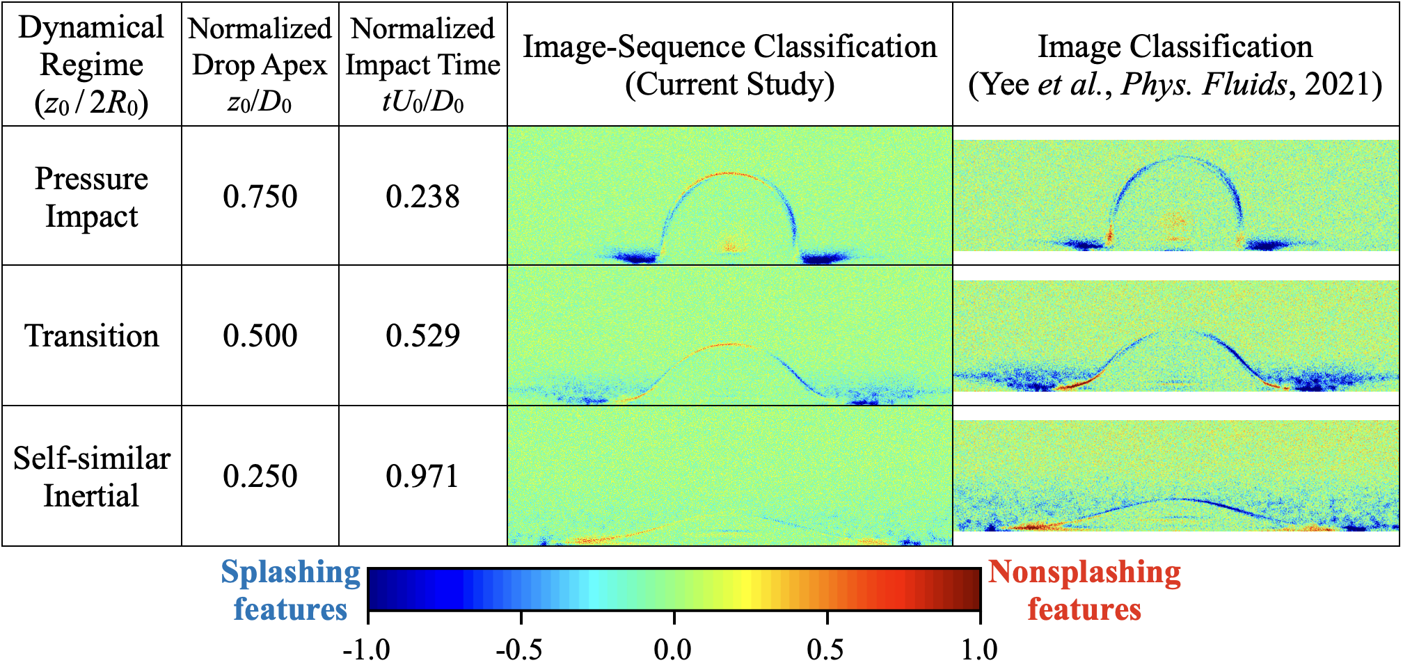
It is important to mention that as $z_{0}/D_{0}$ reduces to $z_{0}/D_{0}\leq 0.500$, the distribution of the splashing features around the contour of the main body becomes less obvious. This is different from the reshaped weight vectors trained using image classification in the study by Yee et al. (2022). In their study, they trained three different FNNs to classify splashing and non-splashing drops using images extracted when $z_{0}/D_{0}=0.750$, 0.500, and 0.250, respectively. As shown in figure 9, the distributions of the splashing and non-splashing features in the reshaped weight vectors trained by Yee et al. (2022) are found at similar pixel positions to those in the current study. Note that in this study, each frame in the image sequences was cropped to $200\times 640$ px², whereas Yee et al. (2022) cropped their images to $160\times 640$ px². However, the distributions are much more obvious for the reshaped vectors trained using only images of $z_{0}/D_{0}=0.250$ than for ${\boldsymbol{w}}_{\mathrm{spl},z_{0}/D_{0}=0.250}$ trained using image sequences. This is because the FNN image classifier can only extract information from a single image, whereas the FNN image-sequence classifier of this study can extract information from seven frames in an image sequence. In other words, the FNN image-sequence classifier can pick and choose the frame from which it wants to extract the information. Although it could possibly miss important morphological features of splashing and non-splashing drops, quantification of the contribution of each frame and the extracted features to the classification by the FNN image-sequence classifier could provide deeper insights into the morphological evolution of splashing and non-splashing drops, which is discussed in the next section.

The importance index for quantifying the contributions of the extracted features in each frame of an image sequence to the classification of the FNN are introduced and discussed in this subsection. As mentioned in § 3.2, the value of $\boldsymbol{w}_{\mathrm{spl},z_{0}/D_{0}}\boldsymbol{\cdot}\boldsymbol{s}_{\mathrm{in},z_{0}/D_{0}}$ for each frame shows the respective contribution to the computation of $q_{\mathrm{out,spl}}$. Denoted by $q_{\mathrm{out,spl},z_{0}/D_{0}}$, the values of $\boldsymbol{w}_{\mathrm{spl},z_{0}/D_{0}}\boldsymbol{\cdot}\boldsymbol{s}_{\mathrm{in},z_{0}/D_{0}}$ for each value of $z_{0}/D_{0}$ are plotted against $q_{\mathrm{out,spl}}$. In figure 10(a), only the plot for combination 1 is shown, because similar results were obtained for the other data combinations. The black dashed line shows $q_{\mathrm{out,spl}}=0$, which corresponds to the classification threshold $y_{\mathrm{pred,spl}}=0.5$. To the left of this line where $q_{\mathrm{out,spl}}\geq 0$, an image sequence is classified as that of a splashing drop, while to the right of this line where $q_{\mathrm{out,spl}}<0$, an image sequence is classified as that of a non-splashing drop. To identify the importance of each $z_{0}/D_{0}$ for the classification of the FNN, least squares fitting is performed for each $z_{0}/D_{0}$ and shown in figure 10(a) by the dotted lines with the same colours as the respective markers. Along with the values of $q_{\mathrm{out,spl}}$, the values of $q_{\mathrm{out,spl},z_{0}/D_{0}}$ of all $z_{0}/D_{0}$ exhibit an increasing trend, where the slopes of all the fitted lines are positive. Here, we argue that the $z_{0}/D_{0}$ with the slope of the highest value has the most influence on the classification of the FNN. This is because if the slope has a low value, then the value of $q_{\mathrm{out,spl},z_{0}/D_{0}}$ remains constant regardless of the value of $q_{\mathrm{out,spl}}$. In other words, $q_{\mathrm{out,spl},z_{0}/D_{0}}$ is similar regardless of whether the classification is splashing or non-splashing. On the contrary, if the slope has a high value, the change in the value of $q_{\mathrm{out,spl},z_{0}/D_{0}}$ contributes significantly to the change in the value of $q_{\mathrm{out,spl}}$. Thus, the classification of an image sequence as that of a splashing or a non-splashing drop is highly dependent on the value of $q_{\mathrm{out,spl},z_{0}/D_{0}}$.

Here, the slope of a fitted line is introduced as the importance index for quantifying the contribution of each frame in an image sequence to the classification of the FNN. Denoted by $\beta_{z_{0}/D_{0}}$, the slopes of the fitted lines are plotted against $tU_{0}/D_{0}$ for the respective $z_{0}/D_{0}$ for all data combinations in figure 10(b). As can be seen, all data combinations have peak values at $tU_{0}/D_{0}=0.24$ and 0.38, corresponding to $z_{0}/D_{0}=0.750$ and 0.625. These peak values, which range between 0.25 and 0.30, are more than approximately double the values at other $tU_{0}/D_{0}$, which are less than 0.15. This indicates that the two frames at $tU_{0}/D_{0}=0.24$ and 0.38 have significantly more influence on the classification by the FNN than the frames at other $tU_{0}/D_{0}$. This is also why the distributions of the splashing and non-splashing features are most obvious in the reshaped matrices of $\boldsymbol{w}_{\mathrm{spl},z_{0}/D_{0}}$ at $tU_{0}/D_{0}=0.24$ and 0.38, as shown in figure 8. Therefore, the morphological differences between splashing and non-splashing drops are most pronounced at $tU_{0}/D_{0}=0.24$ and 0.38, rather than at the earlier impact time. These findings are interesting because, for human eyes, splashing drops might look more different from non-splashing drops at later impact times.

A question follows from the findings above: why is the morphological difference most pronounced at $tU_{0}/D_{0}=0.24$ and 0.38? The answer can be related to the impact force. Almost all drop impact studies focused on the kinematics or the morphology of a drop during impact, until the recent publication of several studies focusing on drop dynamics, specifically the temporal evolution of the impact force and the shear stress distribution beneath impacting drops (Cheng et al., 2022; Philippi et al., 2016; Sun et al., 2022). Specifically, Gordillo et al. (2018) and Mitchell et al. (2019) reported that although the impact force $F$ increases with increasing $\Rey$, the value of $\hat{F}$, which is $F$ normalized by $\rho U_{0}^{2}D_{0}^{2}$, decreases with increasing $\Rey$. Nevertheless, for inertia-dominated drop impacts, the transient normalized impact force profile can be approximated as

where $c$ and $\tau$ are constants, with $c^{2}/\tau=1000\pi/243$ and $1/\tau=10/3$, according to Mitchell et al. (2019). They also reported that the magnitude of the normalized peak impact force is approximately 0.85 and occurs at approximately $tU_{0}/D_{0}=0.15$ when the side walls of the drop are perpendicular to the impacted surface. This is consistent with the present study, because careful observation of the examples of the image sequences in figure 4 shows that the side walls of the drops are perpendicular to the impact surface in the range $0.110<tU_{0}/D_{0}<0.238$ when $0.750<z_{0}/D_{0}<0.875$. For comparison with the $\beta_{z_{0}/D_{0}}$ values, the line profile of $\hat{F}$ proposed by Mitchell et al. (2019) is plotted as the grey dashed line in figure 10(b). As can be seen, the $tU_{0}/D_{0}$ of the peak values of $\beta_{z_{0}/D_{0}}$ are almost immediately after $tU_{0}/D_{0}=0.15$, indicating that the morphological differences between splashing and non-splashing drops are most pronounced after the peak normalized impact force $\hat{F}$ has been exerted on the surface. Since a splashing drop has a higher $U_{0}$ than a non-splashing drop, the peak non-normalized impact force $F$ exerted by a splashing drop is greater than that exerted by a non-splashing drop.

Similar to the trend of $\hat{F}$, after reaching peak values at $tU_{0}/D_{0}=0.238$ and 0.375, $\beta_{z_{0}/D_{0}}$ decreases until $tU_{0}/D_{0}=0.971$. However, $\beta$ slightly increases at $tU_{0}/D_{0}=1.473$, because the lamella of a non-splashing drop develops into a film thicker than that of a splashing drop, as mentioned in § 3.3. In particular, at $tU_{0}/D_{0}=1.473$, when $z_{0}/D_{0}$ decreases to 0.125, this difference in terms of the lamella is the most obvious, and thus could easily be picked up by the FNN. To check this reasoning, the contributions of splashing and non-splashing features to the computation of $q_{\mathrm{out,spl},z_{0}/D_{0}}$ were analysed. Since the negative values in a $\boldsymbol{w}_{\mathrm{spl},z_{0}/D_{0}}$ vector correspond to the features of a splashing drop, the contribution of the splashing features can be computed by summing the products of the elements of $\boldsymbol{w}_{\mathrm{spl},z_{0}/D_{0}}$ that have negative values with the corresponding pixel positions in an image. Similarly, the contribution of the non-splashing features can be computed by summing the products of the elements of $\boldsymbol{w}_{\mathrm{spl},z_{0}/D_{0}}$ that have positive values with the corresponding pixel positions in an image. Thus, let $q_{\mathrm{out,spl},z_{0}/D_{0},\mathrm{neg}}$ and $q_{\mathrm{out,spl},z_{0}/D_{0},\mathrm{pos}}$ be the contributions of the splashing and non-splashing features, respectively, to $q_{\mathrm{out,spl},z_{0}/D_{0}}$:

The values of $q_{\mathrm{out,spl},z_{0}/D_{0},\mathrm{neg}}$ are plotted against $q_{\mathrm{out,spl}}$ of test image sequences of combination 1 in figure 11(a). Only the plots for combination 1 are shown, because similar results were obtained for the other data combinations. Similar to figure 10(a), least squares fitting is performed for each $z_{0}/D_{0}$ and shown by the dotted lines with the same colours as the respective markers. Denoted by $\beta_{\mathrm{neg}}$, the slopes of the fitted lines are plotted against $tU_{0}/D_{0}$ for the respective $z_{0}/D_{0}$ for all data combinations in figure 11(b). As can be seen, the value of $\beta_{\mathrm{neg}}$ fits almost perfectly with the trend of $\hat{F}$, even for $tU_{0}/D_{0}=1.473$. This indicates that the splashing features, which include the contour of the main body and the lifted lamella, are dominated by the impact force. An explanation of the contribution of the non-splashing features can be found in appendix A.

References

- Abadi et al. (2016) Abadi, Martín, Barham, Paul, Chen, Jianmin, Chen, Zhifeng, Davis, Andy, Dean, Jeffrey, Devin, Matthieu, Ghemawat, Sanjay, Irving, Geoffrey, Isard, Michael & others 2016 Tensorflow: A system for large-scale machine learning. In 12th USENIX Symposium on Operating Systems Design and Implementation (OSDI 16), pp. 265–283.
- Adadi & Berrada (2018) Adadi, Amina & Berrada, Mohammed 2018 Peeking inside the black-box: a survey on explainable artificial intelligence (XAI). IEEE Access 6, 52138–52160.
- Arrieta et al. (2020) Arrieta, Alejandro Barredo, Díaz-Rodríguez, Natalia, Del Ser, Javier, Bennetot, Adrien, Tabik, Siham, Barbado, Alberto, García, Salvador, Gil-López, Sergio, Molina, Daniel, Benjamins, Richard, Chatila, Raja & Herrera, Francisco 2020 Explainable artificial intelligence (XAI): Concepts, taxonomies, opportunities and challenges toward responsible AI. Information Fusion 58, 82–115.
- Breitenbach et al. (2018) Breitenbach, Jan, Roisman, Ilia V & Tropea, Cameron 2018 From drop impact physics to spray cooling models: a critical review. Experiments in Fluids 59 (3), 1–21.
- Brunton et al. (2021) Brunton, Steven L, Nathan Kutz, J, Manohar, Krithika, Aravkin, Aleksandr Y, Morgansen, Kristi, Klemisch, Jennifer, Goebel, Nicholas, Buttrick, James, Poskin, Jeffrey, Blom-Schieber, Adriana W & others 2021 Data-driven aerospace engineering: reframing the industry with machine learning. AIAA Journal 59 (8), 2820–2847.
- Brunton et al. (2020) Brunton, Steven L, Noack, Bernd R & Koumoutsakos, Petros 2020 Machine learning for fluid mechanics. Annual Review of Fluid Mechanics 52, 477–508.
- Burzynski et al. (2020) Burzynski, David A, Roisman, Ilia V & Bansmer, Stephan E 2020 On the splashing of high-speed drops impacting a dry surface. Journal of Fluid Mechanics 892.
- Cheng et al. (2022) Cheng, Xiang, Sun, Ting-Pi & Gordillo, Leonardo 2022 Drop impact dynamics: Impact force and stress distributions. Annual Review of Fluid Mechanics 54, 57–81.
- Clanet et al. (2004) Clanet, Christophe, Béguin, Cédric, Richard, Denis & Quéré, David 2004 Maximal deformation of an impacting drop. Journal of Fluid Mechanics 517, 199–208.
- Colvert et al. (2018) Colvert, Brendan, Alsalman, Mohamad & Kanso, Eva 2018 Classifying vortex wakes using neural networks. Bioinspiration & Biomimetics 13 (2), 025003.
- Dickerson et al. (2022) Dickerson, Andrew K, Alam, MD Erfanul, Buckelew, Jacob, Boyum, Nicholas & Turgut, Damla 2022 Predictive modeling of drop impact force on concave targets. Physics of Fluids 34 (10), 102112.
- Eggers et al. (2010) Eggers, Jens, Fontelos, Marco A, Josserand, Christophe & Zaleski, Stéphane 2010 Drop dynamics after impact on a solid wall: theory and simulations. Physics of Fluids 22 (6), 062101.
- Erichson et al. (2020) Erichson, N Benjamin, Mathelin, Lionel, Yao, Zhewei, Brunton, Steven L, Mahoney, Michael W & Kutz, J Nathan 2020 Shallow neural networks for fluid flow reconstruction with limited sensors. Proceedings of the Royal Society A 476 (2238), 20200097.
- Fernández-Raga et al. (2017) Fernández-Raga, María, Palencia, Covadonga, Keesstra, Saskia, Jordán, Antonio, Fraile, Roberto, Angulo-Martínez, Marta & Cerdà, Artemi 2017 Splash erosion: A review with unanswered questions. Earth-Science Reviews 171, 463–477.
- Fukami et al. (2019) Fukami, Kai, Fukagata, Koji & Taira, Kunihiko 2019 Super-resolution reconstruction of turbulent flows with machine learning. Journal of Fluid Mechanics 870, 106–120.
- Gilet & Bourouiba (2015) Gilet, Tristan & Bourouiba, Lydia 2015 Fluid fragmentation shapes rain-induced foliar disease transmission. Journal of the Royal Society Interface 12 (104), 20141092.
- Glorot & Bengio (2010) Glorot, Xavier & Bengio, Yoshua 2010 Understanding the difficulty of training deep feedforward neural networks. In Proceedings of the Thirteenth International Conference on Artificial Intelligence and Statistics, pp. 249–256. JMLR Workshop and Conference Proceedings.
- Gordillo & Riboux (2019) Gordillo, José Manuel & Riboux, Guillaume 2019 A note on the aerodynamic splashing of droplets. Journal of Fluid Mechanics 871.
- Gordillo et al. (2019) Gordillo, José Manuel, Riboux, Guillaume & Quintero, Enrique S 2019 A theory on the spreading of impacting droplets. Journal of Fluid Mechanics 866, 298–315.
- Gordillo et al. (2018) Gordillo, Leonardo, Sun, Ting-Pi & Cheng, Xiang 2018 Dynamics of drop impact on solid surfaces: evolution of impact force and self-similar spreading. Journal of Fluid Mechanics 840, 190–214.
- Güera & Delp (2018) Güera, David & Delp, Edward J 2018 Deepfake video detection using recurrent neural networks. In 2018 15th IEEE International Conference on Advanced Video and Signal Based Surveillance (AVSS), pp. 1–6. IEEE.
- Hatakenaka et al. (2019) Hatakenaka, Ryuta, Breitenbach, Jan, Roisman, Ilia V, Tropea, Cameron & Tagawa, Yoshiyuki 2019 Magic carpet breakup of a drop impacting onto a heated surface in a depressurized environment. International Journal of Heat and Mass Transfer 145, 118729.
- He et al. (2016) He, Kaiming, Zhang, Xiangyu, Ren, Shaoqing & Sun, Jian 2016 Deep residual learning for image recognition. In Proceedings of the IEEE Conference on Computer Vision and Pattern Recognition, pp. 770–778.
- Hou et al. (2019) Hou, Wei, Darakananda, Darwin & Eldredge, Jeff D 2019 Machine-learning-based detection of aerodynamic disturbances using surface pressure measurements. AIAA Journal 57 (12), 5079–5093.
- Josserand & Thoroddsen (2016) Josserand, Christophe & Thoroddsen, Sigurdur T 2016 Drop impact on a solid surface. Annual Review of Fluid Mechanics 48, 365–391.
- Juarez et al. (2012) Juarez, Gabriel, Gastopoulos, Thomai, Zhang, Yibin, Siegel, Michael L & Arratia, Paulo E 2012 Splash control of drop impacts with geometric targets. Physical Review E 85 (2), 026319.
- Kim et al. (2023) Kim, Hyojin, Kim, Junhyuk & Lee, Changhoon 2023 Interpretable deep learning for prediction of prandtl number effect in turbulent heat transfer. Journal of Fluid Mechanics 955, A14.
- Kim et al. (2021) Kim, Hyojin, Kim, Junhyuk, Won, Sungjin & Lee, Changhoon 2021 Unsupervised deep learning for super-resolution reconstruction of turbulence. Journal of Fluid Mechanics 910, A29.
- Kim & Lee (2020a) Kim, Junhyuk & Lee, Changhoon 2020a Deep unsupervised learning of turbulence for inflow generation at various reynolds numbers. Journal of Computational Physics 406, 109216.
- Kim & Lee (2020b) Kim, Junhyuk & Lee, Changhoon 2020b Prediction of turbulent heat transfer using convolutional neural networks. Journal of Fluid Mechanics 882, A18.
- Kluyver et al. (2016) Kluyver, Thomas, Ragan-Kelley, Benjamin, Pérez, Fernando, Granger, Brian E, Bussonnier, Matthias, Frederic, Jonathan, Kelley, Kyle, Hamrick, Jessica B, Grout, Jason, Corlay, Sylvain, , Ivanov, Paul, Avilah, Damián, Abdallai, Safai & Willingm, Carol 2016 Jupyter notebooks-a publishing format for reproducible computational workflows. In Positioning and Power in Academic Publishing: Players, Agents and Agendas (ed. Fernando Loizides & Birgit Schmidt), pp. 87–90. Amsterdam: IOS Press BV.
- Krizhevsky et al. (2012) Krizhevsky, Alex, Sutskever, Ilya & Hinton, Geoffrey E 2012 ImageNet classification with deep convolutional neural networks. Advances in Neural Information Processing Systems 25, 1097–1105.
- Lagubeau et al. (2012) Lagubeau, Guillaume, Fontelos, Marco A, Josserand, Christophe, Maurel, Agnès, Pagneux, Vincent & Petitjeans, Philippe 2012 Spreading dynamics of drop impacts. Journal of Fluid Mechanics 713, 50–60.
- Lavoie et al. (2022) Lavoie, Pierre, Radenac, Emmanuel, Blanchard, Ghislain, Laurendeau, Eric & Villedieu, Philippe 2022 Penalization method for eulerian droplet impingement simulations toward icing applications. AIAA Journal 60 (2), 641–653.
- Li et al. (2020) Li, Jichao, Zhang, Mengqi, Martins, Joaquim RRA & Shu, Chang 2020 Efficient aerodynamic shape optimization with deep-learning-based geometric filtering. AIAA Journal 58 (10), 4243–4259.
- Li et al. (2014) Li, Mu, Zhang, Tong, Chen, Yuqiang & Smola, Alexander J 2014 Efficient mini-batch training for stochastic optimization. In Proceedings of the 20th ACM SIGKDD International Conference on Knowledge Discovery and Data Mining, pp. 661–670.
- Lin et al. (2022) Lin, Xiaodan, Wang, Qiao, Wu, Yingchun, Yao, Longchao, Xue, Zhiliang & Wu, Xuecheng 2022 3d visualization of droplet splash dynamics with high-speed digital holography. Experiments in Fluids 63 (5), 86.
- Lohse (2022) Lohse, Detlef 2022 Fundamental fluid dynamics challenges in inkjet printing. Annual Review of Fluid Mechanics 54, 349–382.
- Lu et al. (2020) Lu, Peter Y, Kim, Samuel & Soljačić, Marin 2020 Extracting interpretable physical parameters from spatiotemporal systems using unsupervised learning. Physical Review X 10 (3), 031056.
- Ma et al. (2019) Ma, Chih-Yao, Chen, Min-Hung, Kira, Zsolt & AlRegib, Ghassan 2019 Ts-lstm and temporal-inception: Exploiting spatiotemporal dynamics for activity recognition. Signal Processing: Image Communication 71, 76–87.
- Mitchell et al. (2019) Mitchell, Benjamin R, Klewicki, Joseph C, Korkolis, Yannis P & Kinsey, Brad L 2019 The transient force profile of low-speed droplet impact: measurements and model. Journal of Fluid Mechanics 867, 300–322.
- Mundo et al. (1995) Mundo, CHR, Sommerfeld, M & Tropea, Cameron 1995 Droplet-wall collisions: experimental studies of the deformation and breakup process. International journal of multiphase flow 21 (2), 151–173.
- Philippi et al. (2016) Philippi, Julien, Lagrée, Pierre-Yves & Antkowiak, Arnaud 2016 Drop impact on a solid surface: short-time self-similarity. Journal of Fluid Mechanics 795, 96–135.
- Pierzyna et al. (2021) Pierzyna, Maximilian, Burzynski, David A, Bansmer, Stephan E & Semaan, Richard 2021 Data-driven splashing threshold model for drop impact on dry smooth surfaces. Physics of Fluids 33 (12), 123317.
- Prechelt (1998) Prechelt, Lutz 1998 Early stopping-but when? In Neural Networks: Tricks of the Trade, pp. 55–69. Springer.
- Riboux & Gordillo (2014) Riboux, Guillaume & Gordillo, José Manuel 2014 Experiments of drops impacting a smooth solid surface: a model of the critical impact speed for drop splashing. Physical Review Letters 113 (2), 024507.
- Riboux & Gordillo (2015) Riboux, Guillaume & Gordillo, José Manuel 2015 The diameters and velocities of the droplets ejected after splashing. Journal of Fluid Mechanics 772, 630–648.
- Riboux & Gordillo (2017) Riboux, Guillaume & Gordillo, José Manuel 2017 Boundary-layer effects in droplet splashing. Physical Review E 96 (1), 013105.
- Rioboo et al. (2001) Rioboo, Romain, Tropea, Cameron & Marengo, Marco 2001 Outcomes from a drop impact on solid surfaces. Atomization and Sprays 11 (2), 155–165.
- Rumelhart et al. (1986) Rumelhart, David E, Hinton, Geoffrey E & Williams, Ronald J 1986 Learning representations by back-propagating errors. Nature 323 (6088), 533–536.
- Sherstinsky (2020) Sherstinsky, Alex 2020 Fundamentals of recurrent neural network (rnn) and long short-term memory (lstm) network. Physica D: Nonlinear Phenomena 404, 132306.
- Sun et al. (2022) Sun, Ting-Pi, Álvarez-Novoa, Franco, Andrade, Klebbert, Gutiérrez, Pablo, Gordillo, Leonardo & Cheng, Xiang 2022 Stress distribution and surface shock wave of drop impact. Nature Communications 13, 1703.
- Tembely et al. (2022) Tembely, Moussa, Vadillo, Damien C, Dolatabadi, Ali & Soucemarianadin, Arthur 2022 A machine learning approach for predicting the maximum spreading factor of droplets upon impact on surfaces with various wettabilities. Processes 10 (6), 1141.
- Thoroddsen et al. (2012) Thoroddsen, Sigurdur T, Takehara, Kohsei & Etoh, TG 2012 Micro-splashing by drop impacts. Journal of Fluid Mechanics 706, 560–570.
- Usawa et al. (2021) Usawa, Masashi, Fujita, Yuta, Tagawa, Yoshiyuki, Riboux, Guillaume & Gordillo, José Manuel 2021 Large impact velocities suppress the splashing of micron-sized droplets. Physical Review Fluids 6 (2), 023605.
- Voulodimos et al. (2018) Voulodimos, Athanasios, Doulamis, Nikolaos, Doulamis, Anastasios & Protopapadakis, Eftychios 2018 Deep learning for computer vision: A brief review. Computational Intelligence and Neuroscience 2018.
- Waite et al. (2015) Waite, Helen, Whitelaw-Weckert, Melanie & Torley, Peter 2015 Grapevine propagation: principles and methods for the production of high-quality grapevine planting material. New Zealand Journal of Crop and Horticultural Science 43 (2), 144–161.
- Wang & Bourouiba (2018) Wang, Y & Bourouiba, Lydia 2018 Unsteady sheet fragmentation: droplet sizes and speeds. Journal of Fluid Mechanics 848, 946–967.
- Yancheshme et al. (2022) Yancheshme, Amir Azimi, Enayati, Saman, Kashcooli, Yaser, Jafari, Reza, Ezzaidi, Hassan & Momen, Gelareh 2022 Dynamic behavior of impinging drops on water repellent surfaces: Machine learning-assisted approach to predict maximum spreading. Experimental Thermal and Fluid Science 139, 110743.
- Yarin (2006) Yarin, Alexander L 2006 Drop impact dynamics: splashing, spreading, receding, bouncing…. Annual Review of Fluid Mechanics 38, 159–192.
- Yee et al. (2023) Yee, Jingzu, Igarashi, Daichi, Miyatake, Shun & Tagawa, Yoshiyuki 2023 Prediction of the morphological evolution of a splashing drop using an encoder–decoder. Machine Learning: Science and Technology 4 (2), 025002.
- Yee et al. (2022) Yee, Jingzu, Yamanaka, Akinori & Tagawa, Yoshiyuki 2022 Image features of a splashing drop on a solid surface extracted using a feedforward neural network. Physics of Fluids 34 (1), 013317.
- Yokoyama et al. (2022) Yokoyama, Yuto, Tanaka, Akane & Tagawa, Yoshiyuki 2022 Droplet impact of blood and blood simulants on a solid surface: Effect of the deformability of red blood cells and the elasticity of plasma. Forensic Science International 331, 111138.
- Yoon et al. (2022) Yoon, Ikroh, Chergui, Jalel, Juric, Damir & Shin, Seungwon 2022 Maximum spreading of droplet-particle collision covering a low Weber number regime and data-driven prediction model. Physics of Fluids 34 (10), 102109.
- Yousif et al. (2023) Yousif, Mustafa Z, Zhang, Meng, Yu, Linqi, Vinuesa, Ricardo & Lim, HeeChang 2023 A transformer-based synthetic-inflow generator for spatially developing turbulent boundary layers. Journal of Fluid Mechanics 957, A6.
- Zhang & Liu (2016) Zhang, Chen & Liu, Hong 2016 Effect of drop size on the impact thermodynamics for supercooled large droplet in aircraft icing. Physics of Fluids 28 (6), 062107.
- Zhang et al. (2022) Zhang, Haixiang, Zhang, Xiwen, Yi, Xian, Du, Yanxia, He, Feng, Niu, Fenglei & Hao, Pengfei 2022 How surface roughness promotes or suppresses drop splash. Physics of Fluids 34 (2), 022111.
- Zhang et al. (2021) Zhang, Haixiang, Zhang, Xiwen, Yi, Xian, He, Feng, Niu, Fenglei & Hao, Pengfei 2021 Reversed role of liquid viscosity on drop splash. Physics of Fluids 33 (5), 052103.