This paper was converted on www.awesomepapers.org from LaTeX by an anonymous user.
Want to know more? Visit the Converter page.

Copula bounds for circular data

Hiroaki Ogata111E-mail: [email protected]
Faculty of Economics and Business Administration, Tokyo Metropolitan University
1-1 Minami-Osawa, Hachioji-shi, Tokyo, Japan 192-0397
Abstract

We propose the extension of Fréchet-Hoeffding copula bounds for circular data. The copula is a powerful tool for describing the dependency of random variables. In two dimensions, the Fréchet-Hoeffding upper (lower) bound indicates the perfect positive (negative) dependence between two random variables. However, for circular random variables, the usual concept of dependency is not accepted because of their periodicity. In this work, we redefine Fréchet-Hoeffding bounds and consider modified Fréchet and Mardia families of copulas for modelling the dependency of two circular random variables. Simulation studies are also given to demonstrate the behavior of the model.
keywords : Circular statistics ; copulas ; Fréchet-Hoeffding bounds

1 Introduction

Circular statistics deals with observations that are represented as points on a unit circle. Directional data is a typical example of this, because a direction is represented as an angle from a certain zero direction. Common examples often cited are: wind direction, river flow direction, and the direction of migrating birds in flight. For a comprehensive explanation of circular statistics, we refer to Fisher (1995), Mardia and Jupp (1999), Jammalamadaka and SenGupta (2001), to name a few.

If the observation is a pair of circular data, usually denoted by (θ,ϕ)𝐂2=[0,2π)2(\theta,\phi)\in\mathbf{C}^{2}=[0,2\pi)^{2}, it is represented as a point on a torus. When we have bivariate data, we can investigate the relationship between them. Although the Pearson correlation coefficient is the representative measure of a relationship between two random variables, it does not work for circular data because of its periodic structure. Many measures of association for circular data have been proposed so far. Section 11.2.2. of Mardia and Jupp (1999) provides a summary of circular-circular correlations.

Another powerful tool for describing the dependency between two random variables is a copula. It is a function rather than a single value and provides much more information regarding dependency. Mathematically speaking, the copula is a joint distribution function on 𝐈2=[0,1]2\mathbf{I}^{2}=[0,1]^{2} whose margins are uniform. For a circular version, Jones et al. (2015) introduced a circular analogue of copula density, called “circulas,” assuming the existence of density function. In this paper, we consider a copula function—not a copula density—for circular data. Because we do not assume the existence of the density function, we can deal with singular copulas. We give special consideration to circular analogues of Fréchet-Hoeffding copula bounds, which are examples of singular copulas. Due to the arbitrary nature of the origin in the circular variable, they are not uniquely specified.

The remainder of the paper is organized as follows: Section 2 provides the definition of the equivalence class of circular copula functions from the aspect of the arbitrariness of the origin point. Section 3 introduces circular analogues of Fréchet-Hoeffding copula bounds. We prove that the following (i) and (ii) are equivalent.

  1. (i)

    The bivariate circular random variables have the circular Fréchet-Hoeffding upper (lower) copula bounds.

  2. (ii)

    Support of the bivariate circular random variables is nondecreasing (nonincreasing) in the sense of mod2π\mod 2\pi.

Section 4 gives a Monte Carlo simulation. We generate observations from the circular version of the Mardia copula family, and investigate their behavior. Section 5 provides our summary and conclusion.

2 Equivalence Class of Circular Copula Functions

A copula is the joint distribution function on 𝐈2=[0,1]2\mathbf{I}^{2}=[0,1]^{2} whose margins are uniform. Sklar’s theorem insists any joint distribution function H(x,y)H(x,y) is written by the copula function C(u,v)C(u,v) and their marginal distribution function F(x)F(x), G(y)G(y), like

H(x,y)=C(F(x),G(y)).\displaystyle H(x,y)=C(F(x),G(y)).

In the case of circular random variables, marginal and joint distribution functions depend on the choice of the zero direction. However, we should not consider the difference caused solely by the difference of the zero direction. This section gives the concept of the equivalence class of circular copula functions in the sense of the arbitrariness of the choice of the zero direction.

First, let us give the definitions of circular distribution functions, quasi-inverses of circular distribution functions and circular joint distribution functions following the style of Definitions 2.3.1, 2.3.6, and 2.3.2. in Nelsen (2006).

Definition 1.

A circular distribution function is a function FF with domain 𝐂=[0,2π)\mathbf{C}=[0,2\pi) such that

  1. 1.

    FF is nondecreasing,

  2. 2.

    F(0)=0F(0)=0 and limθ2πF(θ)=1\lim_{\theta\nearrow 2\pi}F(\theta)=1.

Definition 2.

Let FF be a circular distribution function. Then a quasi-inverse of FF is any function F(1)F^{(-1)} with domain 𝐈\mathbf{I} such that

F(1)(u)=inf{θ|F(θ)u},\displaystyle F^{(-1)}(u)=\inf\{\theta|F(\theta)\geq u\},
Definition 3.

A circular joint distribution function is a function HH with domain 𝐂2\mathbf{C}^{2} such that

  1. 1.

    H(θ2,ϕ2)H(θ2,ϕ1)H(θ1,ϕ2)+H(θ1,ϕ1)0H(\theta_{2},\phi_{2})-H(\theta_{2},\phi_{1})-H(\theta_{1},\phi_{2})+H(\theta_{1},\phi_{1})\geq 0 for any rectangle [θ1,θ2]×[ϕ1,ϕ2]𝐂2[\theta_{1},\theta_{2}]\times[\phi_{1},\phi_{2}]\in\mathbf{C}^{2},

  2. 2.

    H(θ,0)=H(0,ϕ)=0H(\theta,0)=H(0,\phi)=0 and limθ2πlimϕ2πH(θ,ϕ)=1\lim_{\theta\nearrow 2\pi}\lim_{\phi\nearrow 2\pi}H(\theta,\phi)=1.

Now let us extend the domain of FF to 𝐂~=[0,4π)\tilde{\mathbf{C}}=[0,4\pi) in the following way

F~(θ)={F(θ)(0θ<2π)F(θ2π)+1(2πθ<4π)\displaystyle\tilde{F}(\theta)=\left\{\begin{array}[]{ll}F(\theta)&(0\leq\theta<2\pi)\\ F(\theta-2\pi)+1&(2\pi\leq\theta<4\pi)\end{array}\right.

If we change the zero direction to α𝐂\alpha\in\mathbf{C}, its distribution function becomes

Fα(θ)=F~(θ+α)F~(α).\displaystyle F_{\alpha}(\theta)=\tilde{F}(\theta+\alpha)-\tilde{F}(\alpha).

The choice of α\alpha should be arbitrary, so we can define the equivalence class of circular distribution functions {Fα|α𝐂}\{F_{\alpha}|\alpha\in\mathbf{C}\}.

Similarly, we extend the domain of HH to 𝐂~2\tilde{\mathbf{C}}^{2} in the following way

H~(θ,ϕ)\displaystyle\tilde{H}(\theta,\phi)
=\displaystyle= {H(θ,ϕ)(0θ<2π,0ϕ<2π)F(θ)+H(θ,ϕ2π)(0θ<2π,2πϕ<4π)G(ϕ)+H(θ2π,ϕ)(2πθ<4π,0ϕ<2π)1+F(θ2π)+G(ϕ2π)+H(θ2π,ϕ2π)(2πθ<4π,2πϕ<4π)\displaystyle\left\{\begin{array}[]{ll}H(\theta,\phi)&(0\leq\theta<2\pi,0\leq\phi<2\pi)\\ F(\theta)+H(\theta,\phi-2\pi)&(0\leq\theta<2\pi,2\pi\leq\phi<4\pi)\\ G(\phi)+H(\theta-2\pi,\phi)&(2\pi\leq\theta<4\pi,0\leq\phi<2\pi)\\ 1+F(\theta-2\pi)+G(\phi-2\pi)+H(\theta-2\pi,\phi-2\pi)&(2\pi\leq\theta<4\pi,2\pi\leq\phi<4\pi)\end{array}\right.

If we change the zero directions to (α,β)𝐂2(\alpha,\beta)\in\mathbf{C}^{2}, its joint distribution function becomes

Hα,β(θ,ϕ)=H~(θ+α,ϕ+β)H~(α,ϕ+β)H~(θ+α,β)+H~(α,β).\displaystyle H_{\alpha,\beta}(\theta,\phi)=\tilde{H}(\theta+\alpha,\phi+\beta)-\tilde{H}(\alpha,\phi+\beta)-\tilde{H}(\theta+\alpha,\beta)+\tilde{H}(\alpha,\beta).

The choice of (α,β)(\alpha,\beta) should be arbitrary, so we can define the equivalence class of circular joint distribution functions {Hα,β|(α,β)𝐂2}\{H_{\alpha,\beta}|(\alpha,\beta)\in\mathbf{C}^{2}\}.

From Sklar’s theorem, the circular copula function is defined by

Cα,β(u,v)=Hα,β(Fα(1)(u),Gβ(1)(v)).\displaystyle C_{\alpha,\beta}(u,v)=H_{\alpha,\beta}(F_{\alpha}^{(-1)}(u),G_{\beta}^{(-1)}(v)). (1)

The choice of zero directions (α,β)(\alpha,\beta) should be arbitrary, so we can define the equivalence class of circular copula functions {Cα,β|(α,β)𝐂2}\{C_{\alpha,\beta}|(\alpha,\beta)\in\mathbf{C}^{2}\}.

3 Circular Fréchet-Hoeffding copula bounds

A copula is known to have both upper and lower bounds. That is, for every (u,v)𝐈2(u,v)\in\mathbf{I}^{2},

W(u,v):=max(u+v1,0)C(u,v)min(u,v)=:M(u,v).\displaystyle W(u,v):=\max(u+v-1,0)\leq C(u,v)\leq\min(u,v)=:M(u,v).

The bounds M(u,v)M(u,v) and W(u,v)W(u,v) are themselves copulas and are called Fréchet-Hoeffding upper bounds and Fréchet-Hoeffding lower bounds, respectively.

Here, we introduce the concept of a nondecreasing (nonincreasing) set in 𝐑¯2=(,)2\bar{\mathbf{R}}^{2}=(-\infty,\infty)^{2}.

Definition 4 (Definition 2.5.1 in Nelsen (2006)).

A subset SS of 𝐑¯2\bar{\mathbf{R}}^{2} is nondecreasing if for any (x,y)(x,y) and (u,v)(u,v) in SS, x<ux<u implies yvy\leq v. Similarly, a subset SS of 𝐑¯2\bar{\mathbf{R}}^{2} is nonincreasing if for any (x,y)(x,y) and (u,v)(u,v) is SS, x<ux<u implies yvy\geq v.

The example of a nondecreasing set is given in Figure 1.

Refer to caption
Figure 1: Nondecreasing set

If the pair of random variables (X,Y)(X,Y) have a Fréchet-Hoeffding upper (lower) bound, then the support of (X,Y)(X,Y) is nondecreasing (nonincreasing). See Theorems 2.5.4 and 2.5.5 of Nelsen (2006). In this sense, a Fréchet-Hoeffding upper (lower) bound indicates the perfect positive (negative) dependence between XX and YY.

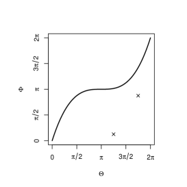
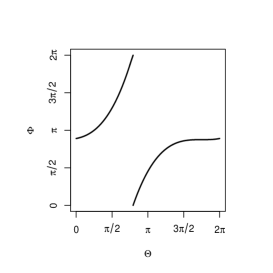
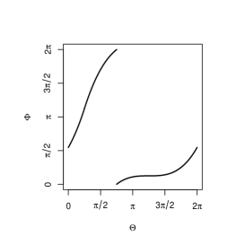
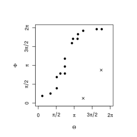
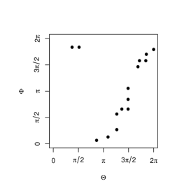
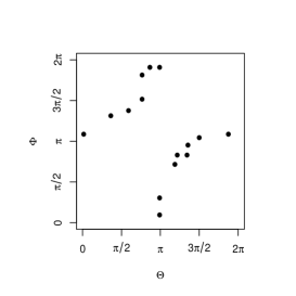
Now let us consider the pair of circular (angular) random variables (Θ,Φ)𝐂2(\Theta,\Phi)\in\mathbf{C}^{2}. When (Θ,Φ)(\Theta,\Phi) has perfect positive dependence, its support should be like the examples shown in the left column of Figure 2. The upper figures are for a continuous circular random variable and the lower figures are for a discrete variable. The figures in the middle and right columns are redrawings of those in the left column when we regard (5π/4,π/8)(5\pi/4,\pi/8) and (7π/4,7π/8)(7\pi/4,7\pi/8) as zero directions (indicated by cross marks in the figures in the left column), respectively. Due to the arbitrary nature of the zero directions, the all support plots in Figure 2 should indicate perfect positive dependence.

Refer to caption
Refer to caption
Refer to caption
Refer to caption
Refer to caption
Refer to caption
Figure 2: Supports of perfect positive dependent circular random variables. The upper figures are for a continuous random variable and the lower figures are for a discrete random variable. The middle and right columns are redrawings of those in the left column when we regard (5π/4,π/8)(5\pi/4,\pi/8) and (7π/4,7π/8)(7\pi/4,7\pi/8) as zero directions (indicated by cross marks in the figures in the left column), respectively.

Now, we give the equivalence class of the circular Fréchet-Hoeffding copula upper bound in the following theorem.

Theorem 1 (Circular Fréchet-Hoeffding copula upper bound).

Let 0a10\leq a\leq 1. The equivalence class of the circular Fréchet-Hoeffding copula upper bound is given by

Ma(u,v)={min(u,va)(u,v)[0,1a]×[a,1]min(u+a1,v)(u,v)[1a,1]×[0,a]max(u+v1,0)otherwise.\displaystyle M_{a}(u,v)=\left\{\begin{array}[]{ll}\min(u,v-a)&(u,v)\in[0,1-a]\times[a,1]\\ \min(u+a-1,v)&(u,v)\in[1-a,1]\times[0,a]\\ \max(u+v-1,0)&\mbox{otherwise}\end{array}\right..

Proof is given in the Appendix.

The copula Ma(u,v)M_{a}(u,v) is introduced in Exercise 3.9 of Nelsen (2006). It is the joint distribution function when the probability mass is uniformly distributed on two line segments, one joining (0,a)(0,a) to (1a,1)(1-a,1) with mass 1a1-a, and the other joining (1a,0)(1-a,0) to (1,a)(1,a) with mass aa. Theorem 1 clarifies this MaM_{a} corresponds to the circular Fréchet-Hoeffding copula upper bound.

We can also find the equivalence class of the circular Fréchet-Hoeffding copula lower bound in the following theorem.

Theorem 2 (Circular Fréchet-Hoeffding copula lower bound).

Let 0a10\leq a\leq 1. The equivalence class of the circular Fréchet-Hoeffding copula lower bound is given by

Wa(u,v)={max(u+va,0)(u,v)[0,a]2max(u+v1,a)(u,v)[a,1]2min(u,v)otherwise\displaystyle W_{a}(u,v)=\left\{\begin{array}[]{ll}\max(u+v-a,0)&(u,v)\in[0,a]^{2}\\ \max(u+v-1,a)&(u,v)\in[a,1]^{2}\\ \min(u,v)&\mbox{otherwise}\end{array}\right.

Proof is omitted because it is similar to that of Theorem 1.

The copula Wa(u,v)W_{a}(u,v) is introduced in Example 3.4 of Nelsen (2006). It is the joint distribution function when the probability mass is uniformly distributed on two line segments, one joining (0,a)(0,a) to (a,0)(a,0) with mass aa, and the other joining (a,1)(a,1) to (1,a)(1,a) with mass 1a1-a.

When describing the dependency between Θ\Theta and Φ\Phi, their periodic structure must be considered. Fisher and Lee (1983) proposed the complete dependence between Θ\Theta and Φ\Phi as

ΦΘ+α0mod(2π),positive association\displaystyle\Phi\equiv\Theta+\alpha_{0}\qquad\mod(2\pi),\qquad\mbox{positive association} (2)
ΦΘ+α0mod(2π),negative association\displaystyle\Phi\equiv-\Theta+\alpha_{0}\qquad\mod(2\pi),\qquad\mbox{negative association} (3)

where α0\alpha_{0} is an arbitrary fixed direction. If we use 𝐂2\mathbf{C}^{2} display, the supports of (2) are expressed as in Figure 3.
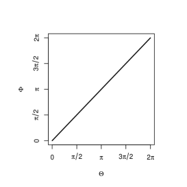
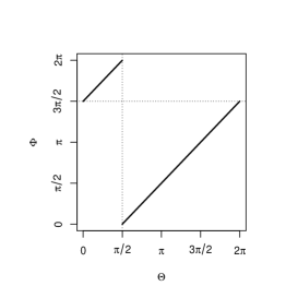
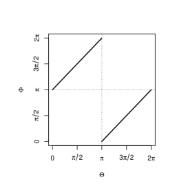
Refer to caption
Refer to caption
Refer to caption
Refer to caption
Refer to caption
Refer to caption
Figure 3: Perfect positive dependence in the sense of Fisher and Lee (1983) with α0=0\alpha_{0}=0 (left), α0=3π/2\alpha_{0}=3\pi/2 (middle), α0=π\alpha_{0}=\pi (right). Upper is for continuous and lower is for discrete.

Because of arbitrary nature of α0\alpha_{0}, not only the left column but also the middle and right columns indicate complete positive dependence. Figure 3 is the special case of Figure 2. Therefore, the circular perfect dependence with the concept of nondecreasing (nonincreasing) set can be considered as the generalization of complete dependence in the sense of Fisher and Lee (1983).

4 Monte Carlo Simulations

In this section, we consider the copula

Cγ,a,b(u,v)=γ2(1+γ)2Ma(u,v)+(1γ2)Π(u,v)+γ2(1γ)2Wb(u,v)\displaystyle C_{\gamma,a,b}(u,v)=\frac{\gamma^{2}(1+\gamma)}{2}M_{a}(u,v)+(1-\gamma^{2})\Pi(u,v)+\frac{\gamma^{2}(1-\gamma)}{2}W_{b}(u,v) (4)
(γ,a,b)[1,1]×𝐈×𝐈.\displaystyle(\gamma,a,b)\in[-1,1]\times\mathbf{I}\times\mathbf{I}.

Here, Ma(u,v)M_{a}(u,v), Wb(u,v)W_{b}(u,v) are the copulas introduced in Theorems 1, 2, and Π(u,v):=uv\Pi(u,v):=uv is an independent copula. This is a linear combination of these three copulas and an analog to the model in Mardia (1970). The parameter γ\gamma controls the weights of these three copulas, and γ=1,0,1\gamma=1,0,-1 correspond MaM_{a} (perfect positive dependence), Π\Pi (independent), WbW_{b} (perfect negative dependence), respectively.

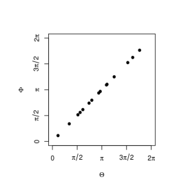
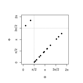
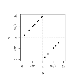
Now we generate a random circular bivariate sample (θi,ϕi)i=1,,500(\theta_{i},\phi_{i})_{i=1,\ldots,500} from (4). Both marginals are set to a Cardioid distribution, whose distribution function is given by

FCa(θ)=ρπsin(θμ)+θ2π+ρπsinμ.\displaystyle F_{\mathrm{Ca}}(\theta)=\frac{\rho}{\pi}\sin(\theta-\mu)+\frac{\theta}{2\pi}+\frac{\rho}{\pi}\sin\mu.

The parameters for marginals are set to ρF=0.1\rho_{F}=0.1, μF=π\mu_{F}=\pi for θ\theta and ρG=0.3\rho_{G}=0.3, μG=π/3\mu_{G}=\pi/3 for ϕ\phi. Figure 4 shows the simulated circular bivariate plots with γ=0.7\gamma=-0.7 (upper left), 0.5-0.5 (upper middle), 0.3-0.3 (upper right), 0.30.3 (lower left), 0.50.5 (lower middle), 0.70.7 (lower right). When γ\gamma is close to 11 and 1-1, (4) is close to MaM_{a} and WbW_{b}, which are singular copulas. When γ=±0.7\gamma=\pm 0.7, we can clearly see the singular components in the plots.

Refer to caption
Refer to caption
Refer to caption
Refer to caption
Refer to caption
Refer to caption
Figure 4: Simulated circular bivariate plots from the model (4). The sample size is 500500. The marginal for θ\theta is a Cardioid distribution with ρF=0.1\rho_{F}=0.1, μF=π\mu_{F}=\pi, and the marginal for ϕ\phi is a Cardioid distribution with ρG=0.3\rho_{G}=0.3, μG=π/3\mu_{G}=\pi/3. The parameters aa and bb are fixed to 0.70.7 and 0.40.4, respectively. The parameter γ\gamma is set to 0.7-0.7 (upper left), 0.5-0.5 (upper middle), 0.3-0.3 (upper right), 0.30.3 (lower left), 0.50.5 (lower middle), 0.70.7 (lower right).

5 Summary and Conclusions

We considered the equivalence class of univariate and bivariate circular distribution functions ascribed to the arbitrary nature of the origin point. Then, we introduced the equivalence class of circular copula functions with Sklar’s theorem. Using the concept of the equivalence class of circular copula functions, we introduced circular analogues of Fréchet-Hoeffding copula upper and lower bounds. We explained they are the generalizations of complete positive and negative dependence in the sense of Fisher and Lee (1983). We also introduced the circular analogue of Mardia’s copula model and simulated a dataset following this model. When the model is close to its extremes, we can find the singular components in the plots.

Appendix

Proof of Theorem 1

Let

H(θ,ϕ)=M(F(θ),G(ϕ))=min(F(θ),G(ϕ)).\displaystyle H(\theta,\phi)=M(F(\theta),G(\phi))=\min(F(\theta),G(\phi)).

Fix arbitrary zero directions (α,β)𝐂(\alpha,\beta)\in\mathbf{C}. From the discussion in Section 2, the circular Fréchet-Hoeffding copula upper bound is

Cα,β(u,v)\displaystyle C_{\alpha,\beta}(u,v)
=\displaystyle= Hα,β(Fα(1)(u),Gβ(1)(v))\displaystyle H_{\alpha,\beta}(F^{(-1)}_{\alpha}(u),G^{(-1)}_{\beta}(v))
=\displaystyle= H~(Fα(1)(u)+α,Gβ(1)(v)+β)H~(α,Gβ(1)(v)+β)H~(Fα(1)(u)+α,β)+H~(α,β).\displaystyle\tilde{H}(F^{(-1)}_{\alpha}(u)+\alpha,G^{(-1)}_{\beta}(v)+\beta)-\tilde{H}(\alpha,G^{(-1)}_{\beta}(v)+\beta)-\tilde{H}(F^{(-1)}_{\alpha}(u)+\alpha,\beta)+\tilde{H}(\alpha,\beta).

When (Θ,Φ)(\Theta,\Phi) is discrete, (u,v)(u,v) is restricted on RanFα×RanGβ\mathrm{Ran}F_{\alpha}\times\mathrm{Ran}G_{\beta}. Now, let us divide 𝐈2\mathbf{I}^{2} into the following four regions:

𝐈1={(u,v)|Fα(1)(u)+α<2π,Gβ(1)(v)+β<2π}={(u,v)|u<1F(α),v<1G(β)}\displaystyle\mathbf{I}_{1}=\{(u,v)\ |\ F^{(-1)}_{\alpha}(u)+\alpha<2\pi,\ G^{(-1)}_{\beta}(v)+\beta<2\pi\}=\{(u,v)\ |\ u<1-F(\alpha),\ v<1-G(\beta)\}
𝐈2={(u,v)|Fα(1)(u)+α<2π,Gβ(1)(v)+β2π}={(u,v)|u<1F(α),v1G(β)}\displaystyle\mathbf{I}_{2}=\{(u,v)\ |\ F^{(-1)}_{\alpha}(u)+\alpha<2\pi,\ G^{(-1)}_{\beta}(v)+\beta\geq 2\pi\}=\{(u,v)\ |\ u<1-F(\alpha),\ v\geq 1-G(\beta)\}
𝐈3={(u,v)|Fα(1)(u)+α2π,Gβ(1)(v)+β<2π}={(u,v)|u1F(α),v<1G(β)}\displaystyle\mathbf{I}_{3}=\{(u,v)\ |\ F^{(-1)}_{\alpha}(u)+\alpha\geq 2\pi,\ G^{(-1)}_{\beta}(v)+\beta<2\pi\}=\{(u,v)\ |\ u\geq 1-F(\alpha),\ v<1-G(\beta)\}
𝐈4={(u,v)|Fα(1)(u)+α2π,Gβ(1)(v)+β2π}={(u,v)|u1F(α),v1G(β)}\displaystyle\mathbf{I}_{4}=\{(u,v)\ |\ F^{(-1)}_{\alpha}(u)+\alpha\geq 2\pi,\ G^{(-1)}_{\beta}(v)+\beta\geq 2\pi\}=\{(u,v)\ |\ u\geq 1-F(\alpha),\ v\geq 1-G(\beta)\}

First, for (u,v)𝐈1(u,v)\in\mathbf{I}_{1},

Cα,β(u,v)\displaystyle C_{\alpha,\beta}(u,v)
=\displaystyle= H(Fα(1)(u)+α,Gβ(1)(v)+β)H(α,Gβ(1)(v)+β)H(Fα(1)(u)+α,β)+H(α,β)\displaystyle H(F^{(-1)}_{\alpha}(u)+\alpha,G^{(-1)}_{\beta}(v)+\beta)-H(\alpha,G^{(-1)}_{\beta}(v)+\beta)-H(F^{(-1)}_{\alpha}(u)+\alpha,\beta)+H(\alpha,\beta)
=\displaystyle= min{F(Fα(1)(u)+α),G(Gβ(1)(v)+β)}min{F(α),G(Gβ(1)(v)+β)}\displaystyle\min\{F(F^{(-1)}_{\alpha}(u)+\alpha),G(G^{(-1)}_{\beta}(v)+\beta)\}-\min\{F(\alpha),G(G^{(-1)}_{\beta}(v)+\beta)\}
min{F(Fα(1)(u)+α),G(β)}+min{F(α),G(β)}\displaystyle-\min\{F(F^{(-1)}_{\alpha}(u)+\alpha),G(\beta)\}+\min\{F(\alpha),G(\beta)\}

Here,

F(Fα(1)(u)+α)=Fα(Fα(1)(u))+F(α)=u+F(α)\displaystyle F(F^{(-1)}_{\alpha}(u)+\alpha)=F_{\alpha}(F^{(-1)}_{\alpha}(u))+F(\alpha)=u+F(\alpha)
G(Gβ(1)(v)+β)=Gβ(Gβ(1)(v))+G(β)=v+G(β).\displaystyle G(G^{(-1)}_{\beta}(v)+\beta)=G_{\beta}(G^{(-1)}_{\beta}(v))+G(\beta)=v+G(\beta).

Therefore,

Cα,β(u,v)=\displaystyle C_{\alpha,\beta}(u,v)= min{u+F(α),v+G(β)}min{F(α),v+G(β)}\displaystyle\min\{u+F(\alpha),v+G(\beta)\}-\min\{F(\alpha),v+G(\beta)\}
min{u+F(α),G(β)}+min{F(α),G(β)}.\displaystyle-\min\{u+F(\alpha),G(\beta)\}+\min\{F(\alpha),G(\beta)\}.

When G(β)>F(α)G(\beta)>F(\alpha), we divide 𝐈1\mathbf{I}_{1} into

𝐈11G={(u,v)𝐈1|uG(β)F(α)}\displaystyle\mathbf{I}^{G}_{1-1}=\{(u,v)\in\mathbf{I}_{1}\ |\ u\leq G(\beta)-F(\alpha)\}
𝐈12G={(u,v)𝐈1|u>G(β)F(α),v>u(G(β)F(α))}\displaystyle\mathbf{I}^{G}_{1-2}=\{(u,v)\in\mathbf{I}_{1}\ |\ u>G(\beta)-F(\alpha),\ v>u-(G(\beta)-F(\alpha))\}
𝐈13G={(u,v)𝐈1|vu(G(β)F(α))}.\displaystyle\mathbf{I}^{G}_{1-3}=\{(u,v)\in\mathbf{I}_{1}\ |\ v\leq u-(G(\beta)-F(\alpha))\}.

When G(β)F(α)G(\beta)\leq F(\alpha), we divide 𝐈1\mathbf{I}_{1} into

𝐈11F={(u,v)𝐈1|vF(α)G(β)}\displaystyle\mathbf{I}^{F}_{1-1}=\{(u,v)\in\mathbf{I}_{1}\ |\ v\leq F(\alpha)-G(\beta)\}
𝐈12F={(u,v)𝐈1|v>F(α)G(β),vu+(F(α)G(β))}\displaystyle\mathbf{I}^{F}_{1-2}=\{(u,v)\in\mathbf{I}_{1}\ |\ v>F(\alpha)-G(\beta),\ v\leq u+(F(\alpha)-G(\beta))\}
𝐈13F={(u,v)𝐈1|v>u+(F(α)G(β))}.\displaystyle\mathbf{I}^{F}_{1-3}=\{(u,v)\in\mathbf{I}_{1}\ |\ v>u+(F(\alpha)-G(\beta))\}.

Then,

Cα,β(u,v)={0(u,v)𝐈11Gu(G(β)F(α))(u,v)𝐈12Gv(u,v)𝐈13G0(u,v)𝐈11Fv(F(α)G(β))(u,v)𝐈12Fu(u,v)𝐈13F\displaystyle\begin{split}C_{\alpha,\beta}(u,v)=\left\{\begin{array}[]{cl}0&\quad(u,v)\in\mathbf{I}^{G}_{1-1}\\[2.84526pt] u-(G(\beta)-F(\alpha))&\quad(u,v)\in\mathbf{I}^{G}_{1-2}\\[2.84526pt] v&\quad(u,v)\in\mathbf{I}^{G}_{1-3}\\[2.84526pt] 0&\quad(u,v)\in\mathbf{I}^{F}_{1-1}\\[2.84526pt] v-(F(\alpha)-G(\beta))&\quad(u,v)\in\mathbf{I}^{F}_{1-2}\\[2.84526pt] u&\quad(u,v)\in\mathbf{I}^{F}_{1-3}\\ \end{array}\right.\end{split} (5)

Second, for (u,v)𝐈2(u,v)\in\mathbf{I}_{2},

Cα,β(u,v)\displaystyle C_{\alpha,\beta}(u,v)
=\displaystyle= [F(α+Fα(1)(u))+H(Fα(1)(u)+α,Gβ(1)(v)+β2π)]\displaystyle[F(\alpha+F^{(-1)}_{\alpha}(u))+H(F^{(-1)}_{\alpha}(u)+\alpha,G^{(-1)}_{\beta}(v)+\beta-2\pi)]
[F(α)+H(α,Gβ(1)(v)+β2π)]H(Fα(1)(u)+α,β)+H(α,β)\displaystyle-[F(\alpha)+H(\alpha,G^{(-1)}_{\beta}(v)+\beta-2\pi)]-H(F^{(-1)}_{\alpha}(u)+\alpha,\beta)+H(\alpha,\beta)
=\displaystyle= [F(α+Fα(1)(u))+min{F(Fα(1)(u)+α),G(Gβ(1)(v)+β2π)}]\displaystyle[F(\alpha+F^{(-1)}_{\alpha}(u))+\min\{F(F^{(-1)}_{\alpha}(u)+\alpha),G(G^{(-1)}_{\beta}(v)+\beta-2\pi)\}]
[F(α)+min{F(α),G(Gβ(1)(v)+β2π)}]min{F(Fα(1)(u)+α),G(β)}\displaystyle-[F(\alpha)+\min\{F(\alpha),G(G^{(-1)}_{\beta}(v)+\beta-2\pi)\}]-\min\{F(F^{(-1)}_{\alpha}(u)+\alpha),G(\beta)\}
+min{F(α),G(β)}\displaystyle+\min\{F(\alpha),G(\beta)\}

Here,

F(Fα(1)(u)+α)=Fα(Fα(1)(u))+F(α)=u+F(α)\displaystyle F(F^{(-1)}_{\alpha}(u)+\alpha)=F_{\alpha}(F^{(-1)}_{\alpha}(u))+F(\alpha)=u+F(\alpha)
G(Gβ(1)(v)+β2π)=Gβ(Gβ(1)(v))Gβ(2πβ)=v(1G(β)).\displaystyle G(G^{(-1)}_{\beta}(v)+\beta-2\pi)=G_{\beta}(G^{(-1)}_{\beta}(v))-G_{\beta}(2\pi-\beta)=v-(1-G(\beta)).

Therefore,

Cα,β(u,v)=\displaystyle C_{\alpha,\beta}(u,v)= u+min{u+F(α),v(1G(β))}min{F(α),v(1G(β))}\displaystyle u+\min\{u+F(\alpha),v-(1-G(\beta))\}-\min\{F(\alpha),v-(1-G(\beta))\}
min{u+F(α),G(β)}+min{F(α),G(β)}\displaystyle-\min\{u+F(\alpha),G(\beta)\}+\min\{F(\alpha),G(\beta)\}

When G(β)>F(α)G(\beta)>F(\alpha), we divide 𝐈2\mathbf{I}_{2} into

𝐈21G={(u,v)𝐈2|uG(β)F(α),v1(G(β)F(α))}\displaystyle\mathbf{I}^{G}_{2-1}=\{(u,v)\in\mathbf{I}_{2}\ |\ u\leq G(\beta)-F(\alpha),\ v\leq 1-(G(\beta)-F(\alpha))\}
𝐈22G={(u,v)𝐈2|u>G(β)F(α),v1(G(β)F(α))}\displaystyle\mathbf{I}^{G}_{2-2}=\{(u,v)\in\mathbf{I}_{2}\ |\ u>G(\beta)-F(\alpha),\ v\leq 1-(G(\beta)-F(\alpha))\}
𝐈23G={(u,v)𝐈2|v>u+{1(G(β)F(α))}}\displaystyle\mathbf{I}^{G}_{2-3}=\{(u,v)\in\mathbf{I}_{2}\ |\ v>u+\{1-(G(\beta)-F(\alpha))\}\,\}
𝐈24G={(u,v)𝐈2|uG(β)F(α), 1(G(β)F(α))<vu+{1(G(β)F(α))}}\displaystyle\mathbf{I}^{G}_{2-4}=\{(u,v)\in\mathbf{I}_{2}\ |\ u\leq G(\beta)-F(\alpha),\ 1-(G(\beta)-F(\alpha))<v\leq u+\{1-(G(\beta)-F(\alpha))\}\,\}
𝐈25G={(u,v)𝐈2|u>G(β)F(α),v>1(G(β)F(α))}.\displaystyle\mathbf{I}^{G}_{2-5}=\{(u,v)\in\mathbf{I}_{2}\ |\ u>G(\beta)-F(\alpha),\ v>1-(G(\beta)-F(\alpha))\}.

When G(β)F(α)G(\beta)\leq F(\alpha), we do not divide 𝐈2\mathbf{I}_{2} further and rename it as 𝐈21F\mathbf{I}^{F}_{2-1}. Then,

Cα,β(u,v)={0(u,v)𝐈21Gu(G(β)F(α))(u,v)𝐈22Gu(u,v)𝐈23Gv{1(G(β)F(α))}(u,v)𝐈24Gu+v1(u,v)𝐈25Gu(u,v)𝐈21F\displaystyle\begin{split}C_{\alpha,\beta}(u,v)=\left\{\begin{array}[]{cl}0&\quad(u,v)\in\mathbf{I}^{G}_{2-1}\\[2.84526pt] u-(G(\beta)-F(\alpha))&\quad(u,v)\in\mathbf{I}^{G}_{2-2}\\[2.84526pt] u&\quad(u,v)\in\mathbf{I}^{G}_{2-3}\\[2.84526pt] v-\{1-(G(\beta)-F(\alpha))\}&\quad(u,v)\in\mathbf{I}^{G}_{2-4}\\[2.84526pt] u+v-1&\quad(u,v)\in\mathbf{I}^{G}_{2-5}\\[2.84526pt] u&\quad(u,v)\in\mathbf{I}^{F}_{2-1}\\ \end{array}\right.\end{split} (6)

Third, for (u,v)𝐈3(u,v)\in\mathbf{I}_{3},

Cα,β(u,v)\displaystyle C_{\alpha,\beta}(u,v)
=\displaystyle= [G(β+Gβ(1)(v))+H(Fα(1)(u)+α2π,Gβ(1)(v)+β)]\displaystyle[G(\beta+G^{(-1)}_{\beta}(v))+H(F^{(-1)}_{\alpha}(u)+\alpha-2\pi,G^{(-1)}_{\beta}(v)+\beta)]
[G(β)+H(Fα(1)(u)+α2π,β)]H(α,Gβ(1)(v)+β)+H(α,β)\displaystyle-[G(\beta)+H(F^{(-1)}_{\alpha}(u)+\alpha-2\pi,\beta)]-H(\alpha,G^{(-1)}_{\beta}(v)+\beta)+H(\alpha,\beta)
=\displaystyle= [G(β+Gβ(1)(v))+min{F(Fα(1)(u)+α2π),G(Gβ(1)(v)+β)}]\displaystyle[G(\beta+G^{(-1)}_{\beta}(v))+\min\{F(F^{(-1)}_{\alpha}(u)+\alpha-2\pi),G(G^{(-1)}_{\beta}(v)+\beta)\}]
[G(β)+min{F(Fα(1)(u)+α2π),G(β)}]min{F(α),G(Gβ(1)(v)+β)}\displaystyle-[G(\beta)+\min\{F(F^{(-1)}_{\alpha}(u)+\alpha-2\pi),G(\beta)\}]-\min\{F(\alpha),G(G^{(-1)}_{\beta}(v)+\beta)\}
+min{F(α),G(β)}.\displaystyle+\min\{F(\alpha),G(\beta)\}.

Here,

F(Fα(1)(u)+α2π)=Fα(Fα(1)(u))Fα(2πα)=u(1F(α))\displaystyle F(F^{(-1)}_{\alpha}(u)+\alpha-2\pi)=F_{\alpha}(F^{(-1)}_{\alpha}(u))-F_{\alpha}(2\pi-\alpha)=u-(1-F(\alpha))
G(Gβ(1)(v)+β)=Gβ(Gβ(1)(v))+G(β)=v+G(β).\displaystyle G(G^{(-1)}_{\beta}(v)+\beta)=G_{\beta}(G^{(-1)}_{\beta}(v))+G(\beta)=v+G(\beta).

Therefore,

Cα,β(u,v)=\displaystyle C_{\alpha,\beta}(u,v)= v+min{u(1F(α)),v+G(β)}min{u(1F(α)),G(β)}\displaystyle v+\min\{u-(1-F(\alpha)),v+G(\beta)\}-\min\{u-(1-F(\alpha)),G(\beta)\}
min{F(α),v+G(β)}+min{F(α),G(β)}\displaystyle-\min\{F(\alpha),v+G(\beta)\}+\min\{F(\alpha),G(\beta)\}

When G(β)>F(α)G(\beta)>F(\alpha), we do not divide 𝐈3\mathbf{I}_{3} further and rename it 𝐈31G\mathbf{I}^{G}_{3-1}. When G(β)F(α)G(\beta)\leq F(\alpha), we divide 𝐈3\mathbf{I}_{3} into

𝐈31F={(u,v)𝐈3|u1(F(α)G(β)),vF(α)G(β)}\displaystyle\mathbf{I}^{F}_{3-1}=\{(u,v)\in\mathbf{I}_{3}\ |\ u\leq 1-(F(\alpha)-G(\beta)),\ v\leq F(\alpha)-G(\beta)\}
𝐈32F={(u,v)𝐈3|u>1(F(α)G(β)),vF(α)G(β),v>u{1(F(α)G(β))}}\displaystyle\mathbf{I}^{F}_{3-2}=\{(u,v)\in\mathbf{I}_{3}\ |\ u>1-(F(\alpha)-G(\beta)),\ v\leq F(\alpha)-G(\beta),\ v>u-\{1-(F(\alpha)-G(\beta))\}\,\}
𝐈33F={(u,v)𝐈3|vu{1(F(α)G(β))}}\displaystyle\mathbf{I}^{F}_{3-3}=\{(u,v)\in\mathbf{I}_{3}\ |\ v\leq u-\{1-(F(\alpha)-G(\beta))\}\,\}
𝐈34F={(u,v)𝐈3|u1(F(α)G(β)),v>F(α)G(β)}\displaystyle\mathbf{I}^{F}_{3-4}=\{(u,v)\in\mathbf{I}_{3}\ |\ u\leq 1-(F(\alpha)-G(\beta)),\ v>F(\alpha)-G(\beta)\}
𝐈35F={(u,v)𝐈3|u>1(F(α)G(β)),v>F(α)G(β)}.\displaystyle\mathbf{I}^{F}_{3-5}=\{(u,v)\in\mathbf{I}_{3}\ |\ u>1-(F(\alpha)-G(\beta)),\ v>F(\alpha)-G(\beta)\}.

Then,

Cα,β(u,v)={v(u,v)𝐈31G0(u,v)𝐈31Fu{1(F(α)G(β))}(u,v)𝐈32Fv(u,v)𝐈33Fv(F(α)G(β))(u,v)𝐈34Fu+v1(u,v)𝐈35F\displaystyle\begin{split}C_{\alpha,\beta}(u,v)=\left\{\begin{array}[]{cl}v&\quad(u,v)\in\mathbf{I}^{G}_{3-1}\\[2.84526pt] 0&\quad(u,v)\in\mathbf{I}^{F}_{3-1}\\[2.84526pt] u-\{1-(F(\alpha)-G(\beta))\}&\quad(u,v)\in\mathbf{I}^{F}_{3-2}\\[2.84526pt] v&\quad(u,v)\in\mathbf{I}^{F}_{3-3}\\[2.84526pt] v-(F(\alpha)-G(\beta))&\quad(u,v)\in\mathbf{I}^{F}_{3-4}\\[2.84526pt] u+v-1&\quad(u,v)\in\mathbf{I}^{F}_{3-5}\\ \end{array}\right.\end{split} (7)

Lastly, for (u,v)𝐈4(u,v)\in\mathbf{I}_{4},

Cα,β(u,v)\displaystyle C_{\alpha,\beta}(u,v)
=\displaystyle= [1+F(Fα(1)(u)+α2π)+G(Gβ(1)(v)+β2π)+H(Fα(1)(u)+α2π,Gβ(1)(v)+β2π)]\displaystyle[1+F(F^{(-1)}_{\alpha}(u)+\alpha-2\pi)+G(G^{(-1)}_{\beta}(v)+\beta-2\pi)+H(F^{(-1)}_{\alpha}(u)+\alpha-2\pi,G^{(-1)}_{\beta}(v)+\beta-2\pi)]
[F(α)+H(α,Gβ(1)(v)+β2π)][G(β)+H(Fα(1)(u)+α2π,β)]+H(α,β)\displaystyle-[F(\alpha)+H(\alpha,G^{(-1)}_{\beta}(v)+\beta-2\pi)]-[G(\beta)+H(F^{(-1)}_{\alpha}(u)+\alpha-2\pi,\beta)]+H(\alpha,\beta)
=\displaystyle= [1+F(Fα(1)(u)+α2π)+G(Gβ(1)(v)+β2π)+min{F(Fα(1)(u)+α2π),G(Gβ(1)(v)+β2π)}]\displaystyle[1+F(F^{(-1)}_{\alpha}(u)+\alpha-2\pi)+G(G^{(-1)}_{\beta}(v)+\beta-2\pi)+\min\{F(F^{(-1)}_{\alpha}(u)+\alpha-2\pi),G(G^{(-1)}_{\beta}(v)+\beta-2\pi)\}]
[F(α)+min{F(α),G(Gβ(1)(v)+β2π)}][G(β)+min{F(Fα(1)(u)+α2π),G(β)}]\displaystyle-[F(\alpha)+\min\{F(\alpha),G(G^{(-1)}_{\beta}(v)+\beta-2\pi)\}]-[G(\beta)+\min\{F(F^{(-1)}_{\alpha}(u)+\alpha-2\pi),G(\beta)\}]
+min{F(α),G(β)}.\displaystyle+\min\{F(\alpha),G(\beta)\}.

Here,

F(Fα(1)(u)+α2π)=Fα(Fα(1)(u))Fα(2πα)=u(1F(α))\displaystyle F(F^{(-1)}_{\alpha}(u)+\alpha-2\pi)=F_{\alpha}(F^{(-1)}_{\alpha}(u))-F_{\alpha}(2\pi-\alpha)=u-(1-F(\alpha))
G(Gβ(1)(v)+β2π)=Gβ(Gβ(1)(v))Gβ(2πβ)=v(1G(β)).\displaystyle G(G^{(-1)}_{\beta}(v)+\beta-2\pi)=G_{\beta}(G^{(-1)}_{\beta}(v))-G_{\beta}(2\pi-\beta)=v-(1-G(\beta)).

Therefore,

Cα,β(u,v)\displaystyle C_{\alpha,\beta}(u,v)
=\displaystyle= u+v1+min{u(1F(α)),v(1G(β))}\displaystyle u+v-1+\min\{u-(1-F(\alpha)),v-(1-G(\beta))\}
min{F(α),v(1G(β))}min{u(1F(α)),G(β)}+min{F(α),G(β)}.\displaystyle-\min\{F(\alpha),v-(1-G(\beta))\}-\min\{u-(1-F(\alpha)),G(\beta)\}+\min\{F(\alpha),G(\beta)\}.

When G(β)>F(α)G(\beta)>F(\alpha), we divide 𝐈4\mathbf{I}_{4} into

𝐈41G={(u,v)𝐈4|vu(G(β)F(α))}\displaystyle\mathbf{I}^{G}_{4-1}=\{(u,v)\in\mathbf{I}_{4}\ |\ v\leq u-(G(\beta)-F(\alpha))\}
𝐈42G={(u,v)𝐈4|v1(G(β)F(α)),v>u(G(β)F(α))}\displaystyle\mathbf{I}^{G}_{4-2}=\{(u,v)\in\mathbf{I}_{4}\ |\ v\leq 1-(G(\beta)-F(\alpha)),\ v>u-(G(\beta)-F(\alpha))\}
𝐈43G={(u,v)𝐈4|v>1(G(β)F(α))}\displaystyle\mathbf{I}^{G}_{4-3}=\{(u,v)\in\mathbf{I}_{4}\ |\ v>1-(G(\beta)-F(\alpha))\}

When G(β)F(α)G(\beta)\leq F(\alpha), we divide 𝐈4\mathbf{I}_{4} into

𝐈41F={(u,v)𝐈4|v>u+(F(α)G(β))}\displaystyle\mathbf{I}^{F}_{4-1}=\{(u,v)\in\mathbf{I}_{4}\ |\ v>u+(F(\alpha)-G(\beta))\}
𝐈42F={(u,v)𝐈4|u1(F(α)G(β)),vu+(F(α)G(β))}\displaystyle\mathbf{I}^{F}_{4-2}=\{(u,v)\in\mathbf{I}_{4}\ |\ u\leq 1-(F(\alpha)-G(\beta)),\ v\leq u+(F(\alpha)-G(\beta))\}
𝐈43F={(u,v)𝐈4|u>1(F(α)G(β))}.\displaystyle\mathbf{I}^{F}_{4-3}=\{(u,v)\in\mathbf{I}_{4}\ |\ u>1-(F(\alpha)-G(\beta))\}.

Then,

Cα,β(u,v)={v(u,v)𝐈41Gu(G(β)F(α))(u,v)𝐈42Gu+v1(u,v)𝐈43Gu(u,v)𝐈41Fv(F(α)G(β))(u,v)𝐈42Fu+v1(u,v)𝐈43F\displaystyle\begin{split}C_{\alpha,\beta}(u,v)=\left\{\begin{array}[]{cl}v&\quad(u,v)\in\mathbf{I}^{G}_{4-1}\\[2.84526pt] u-(G(\beta)-F(\alpha))&\quad(u,v)\in\mathbf{I}^{G}_{4-2}\\[2.84526pt] u+v-1&\quad(u,v)\in\mathbf{I}^{G}_{4-3}\\[2.84526pt] u&\quad(u,v)\in\mathbf{I}^{F}_{4-1}\\[2.84526pt] v-(F(\alpha)-G(\beta))&\quad(u,v)\in\mathbf{I}^{F}_{4-2}\\[2.84526pt] u+v-1&\quad(u,v)\in\mathbf{I}^{F}_{4-3}\\ \end{array}\right.\end{split} (8)

From (5)–(8), we find Cα,β(u,v)C_{\alpha,\beta}(u,v) is equivalent to Ma(u,v)M_{a}(u,v) in Theorem 1 by taking

a={1(G(β)F(α))(F(α)G(β))F(α)G(β)(F(α)>G(β)).\displaystyle a=\left\{\begin{array}[]{ll}1-(G(\beta)-F(\alpha))&(F(\alpha)\leq G(\beta))\\ F(\alpha)-G(\beta)&(F(\alpha)>G(\beta))\end{array}\right..

Acknowledgements

Financial support for this research was received from JSPS KAKENHI in the form of grant 18K11193. We would like to thank Editage (www.editage.jp) for English language editing.

References

  • Fisher (1995) Fisher NI (1995) Statistical Analysis of Circular Data. Cambridge University Press.
  • Fisher and Lee (1983) Fisher NI, Lee AJ (1983) A correlation coefficient for circular data. BIOMETRIKA 70:327-332
  • Jammalamadaka and SenGupta (2001) Jammalamadaka SA, SenGupta AS (2001) Topics in circular statistics. World Scientific Publishing Co. New York
  • Jones et al. (2015) Jones MC, Pewsey A, Kato S (2015) On a class of circulas: copulas for circular distributions, ANN I STAT MATH 67:843-862
  • Mardia (1970) Mardia KV (1970). Families of Bivariate Distributions. Hafner Publishing Company, Darien, Connecticut.
  • Mardia and Jupp (1999) Mardia KV, Jupp PE (1999) Directional Statistics. Wiley, Chichester
  • Nelsen (2006) Nelsen, RB (2006) An Introduction to Copulas. Springer.