Copula-based measures of asymmetry between the lower and upper tail probabilities

Proposition 2 implies that $\alpha(u)=0$ for any $u\in[0,0.5]$ if $C(u,u)=\overline{C}(\bar{u},\bar{u})$ for any $u\in[0,0.5]$. Such copulas include the independence copula, Gaussian copula, $t$-copula, Plackett copula and FGM copula. Among well-known Archimedean copulas, Frank copula has a radially symmetric shape and therefore $\alpha(u)=0$ for any $u$.

There exist various copulas for which $\alpha(u)$ is not equal to zero in general. Many Archimedean copulas have asymmetric tails, including Clayton copula, Gumbel copula, Ali-Mikhail-Haq copula and two-parameter BB copulas. In addition, some asymmetric extensions of Gaussian copula and $t$-copula have been proposed recently. Such extensions include the skew-normal copulas and skew-$t$ copulas discussed in Joe (2006) and Yoshiba (2018), for which $\alpha(u)$ is not equal to zero in general. As examples of copulas with asymmetric tails, here we discuss the values of $\alpha(u)$ for the three well-known copulas, namely, Clayton copula, Ali-Mikhail-Haq copula and BB7 copula.

Figure 1(a) plots the values of $\alpha(u)$ as a function of $u$ for four positive values of $\theta$. (For an intuitive understanding of the distributions of Clayton copula, see Figure S1(a) and (b) of Supplementary Material which plot random variates from Clayton copula with the two values of the parameters used in Figure 1.) As is clear from equation (2), $\alpha(0.5)=0$ for any $\theta$. The smaller the value of $u$, the smaller the value of $\alpha(u)$. The figure also suggests that, for a fixed value of $u$, as $\theta$ increases, the value of $\alpha(u)$ approaches zero. The upper tail dependence coefficient of Clayton copula is 0 and the lower tail dependence coefficient is $2^{-1/\theta}$ for $\theta>0$ and $0$ for $\theta\leq 0$. Therefore, for $\theta>0$, Theorem 1 implies that $\alpha(0)=-\infty$, meaning that the lower tail dependence is considerably stronger than the upper one. If $\theta\in[-1,0)$, it follows from Theorem 3 that $\alpha(0)=\infty$.

It follows from Theorem 1 that $\alpha(0)=\log(2-2^{1/\theta})-\delta^{-1}\log 2$.

Figure 2 displays a plot of $\alpha(u)$ with respect to $u$ for four selected values of $(\delta,\theta)$ and that of $\alpha(u)$ with respect to $(\delta,\theta)$ for $u=0.01$. Note that, in Figure 2(a), $\delta=1$ and $\delta=1.94$ imply that the lower tail dependence coefficients are around 0.5 and 0.9, respectively, while $\theta=1.71$ and $\theta=7.27$ suggest that the upper tail dependence coefficients are about 0.5 and 0.7, respectively. (See also Figure S1(g)–(h) of Supplementary Material for plots of random variates from BB7 copula (7) with the three combinations of the parameters in Figure 2(a).) Figure 2(a) suggests that, when both the lower and upper tail dependence coefficients are around 0.5, the values of $\alpha(u)$ are close to zero for any $u$. When the difference between the lower and upper tail dependence coefficients is large, $\alpha(u)$ appears to be monotonic with respect to $u$. It can be seen from Figure 2(b) that the values of $\alpha(0.01)$ monotonically decreases as $\delta$ increases. Also, $\alpha(0.01)$ monotonically increases with $\theta$. The two contours $\alpha(0.01)=0$ and $\alpha(0)=0$ show somewhat similar shapes, implying that $\alpha(0.01)=0$ is a reasonable approximation to $\alpha(0)=0$.

A sample analogue of $\alpha(u)$ based on a sample from a copula is defined as follows.

In Sections 5.1–S1.6, we assume that $(U_{11},U_{21}),$$\ldots,$$(U_{1n},U_{2n})$ is an iid sample from the copula $C(u_{1},u_{2})$. For iid $\mathbb{R}^{2}$-valued random vectors $(X_{11},X_{21})$$,\ldots,$ $(X_{1n},X_{2n})$, if the margins of $X_{11}$ and $X_{21}$ are known to be $F_{1}$ and $F_{2}$, respectively, then $\hat{\alpha}(u)$ can be obtained by replacing $(U_{1j},U_{2j})$ by $(F_{1}(X_{1j}),F_{2}(X_{2j}))$ $(j=1,\ldots,n)$.

The goal of this subsection is to investigate some properties of $\hat{\alpha}(u)$. To achieve this, we first show the following lemma. See Supplementary Material for the proof.

This lemma implies that $\hat{\alpha}(u)$ is a consistent estimator of $\alpha(u)$. Applying this lemma, we obtain the following asymptotic result. The proof is given in Supplementary Material.

We note that the covariance function (8) is monotonically decreasing with respect to $u\vee v$. If $u\vee v=0.5$, then the covariance function (8) reaches the minimum value $2/C(0.5,0.5)$.

An asymptotic interval estimator of $\alpha(u)$ can be obtained by applying the asymptotic results obtained in the previous subsection. Theorem 4 implies that, for fixed $u\in(0,0.5]$,

where $\sigma^{2}(u)=\sigma(u,u)$ and $\sigma(u,u)$ is defined as in equation (8). Since $\sigma(u)$ includes the copula $C$ which is usually not known in practice, we use an estimator of $\sigma(u)$ defined by

It follows from Lemma 1 that $\hat{\sigma}(u)\xrightarrow{a.s.}\sigma(u)$ as $n\rightarrow\infty$. Then we have $\sqrt{n}\{\hat{\alpha}(u)-\alpha(u)\}/\hat{\sigma}(u)\xrightarrow{d}N(0,1)$ as $n\rightarrow\infty$. Hence a $100(1-p)$% nonparametric asymptotic confidence interval for $\alpha(u)$ is

where $z_{p/2}$ satisfies $\mathbb{P}(Z\geq z_{p/2})=p/2$, where $Z\sim N(0,1)$ and $0<p<1$.

Notice that the asymptotic confidence interval (9) is a pointwise one for a fixed value of $u$. If the interest of statistical analysis is to construct an asymptotic confidence band for $\alpha(u)$ for a range of $u$, one can adopt Bonferroni correction. This can be done by replacing $p$ by $p/n$ in the equation (9) for $u\in\mathbb{U}$, where $\mathbb{U}=\{\min(\max(u_{1i},u_{2i}),\max(1-u_{1i},1-u_{2i}))\}_{i=1}^{n}$. Therefore the asymptotic confidence band for $\alpha(u)$ with Bonferroni correction is

where $u_{\min}=\min\mathbb{U}$ and $u_{\max}=\max\mathbb{U}$. Since $\hat{\alpha}(u)$ and $\hat{\sigma}(u)$ are step functions, it suffices to evaluate the bounds of confidence intervals only for $u\in\mathbb{U}$.

Some hypothesis tests can be established based on $\hat{\alpha}(u)$. For a given value of $u=u_{0}$, one can carry out a hypothesis test to test $H_{0}:\alpha(u_{0})=\alpha_{0}$ against $H_{1}:\alpha(u_{0})\neq\alpha_{0}$ by using the asymptotic confidence interval (9). Similarly, an one-sided test for the alternative hypothesis $H_{1}:\alpha(u_{0})>\alpha_{0}$ or $H_{1}:\alpha(u_{0})<\alpha_{0}$ can be derived by modifying the asymptotic confidence interval (9).

If the interest of analysis is to evaluate the values of $\hat{\alpha}(u)$ for multiple values of $u$, one can consider the test $H_{0}:\alpha(u)=\alpha_{0}(u)$ against $H_{1}:\alpha(u)\neq\alpha_{0}(u)$ for $\{u;u=u_{1},\ldots,u_{m}\}$. One example of such tests is based on a asymptotic confidence band based on Bonferroni correction (10). However, since the confidence band based on Bonferroni correction is known to be conservative, especially, for dependent hypotheses, the test based on Bonferroni correction (10) is not powerful in general. Alternatively, the following result can be used to present a test for the multiple values of $u$. See Supplementary Material for the proof.

Substituting $\alpha_{0}(u)$ into $\alpha(u)$ in the test statistic $\bm{a}^{T}\hat{\bm{\Sigma}}^{-1}\bm{a}$, the null hypothesis $\alpha(u)=\alpha_{0}(u)$ is rejected for a large value of $\bm{a}^{T}\hat{\bm{\Sigma}}^{-1}\bm{a}$. In order that $\hat{\bm{\Sigma}}$ becomes invertible, the values of $(u_{1},\ldots,u_{m})$ need to be selected such that $T_{U}(u_{i})<T_{U}(u_{i+1})$ and/or $T_{L}(u_{i})<T_{L}(u_{i+1})$ hold for any $1\leq i\leq m-1$.

The sample analogue of $\alpha(u)$ given in Definition 2 can be calculated on the assumption that the margins of the $\mathbb{R}^{2}$-valued random vector are known. Here we discuss the case in which margins are unknown and empirical distributions are adopted as the margins.

Note that the denominator of the empirical distribution function (11) is defined by $n+1$ rather than $n$ in order to avoid positive bias of $\hat{\alpha}(u)$.

The authors have not yet obtained the asymptotic distribution for $\hat{\alpha}^{*}(u)$. However the following results are available regarding $T_{U}^{*}(u)$ and $T_{L}^{*}(u)$. The proof is straightforward from Fermanian et al. (2004), Tsukahara (2005) and Segers (2012) and therefore omitted.

Confidence intervals for $\alpha^{*}(u)$ can be numerically constructed using the bootstrap method. Hypothesis tests can also be established based on the bootstrap confidence intervals. It should be noted that, in order to calculate $\alpha^{*}(u)$ based on bootstrap samples, $\hat{F}_{1}$ and $\hat{F}_{2}$ in (11) should be calculated based on each bootstrap sample. If $\hat{F}_{1}$ and $\hat{F}_{2}$ are calculated from the original data, the bootstrap confidence intervals become similar to the asymptotic confidence intervals (9) for large $n$.

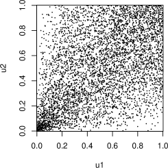
In order to compare the performance of the two proposed sample analogues of $\alpha(u)$ for a large sample size, we consider the following cumulative distribution function

where $F_{j}(x)$ is the cumulative distribution function of the standard Cauchy distribution, i.e., $F_{j}(x)=0.5+\pi^{-1}\arctan x$, and $C_{cl}(u_{1},u_{2};\theta)$ denotes the Clayton copula (5).

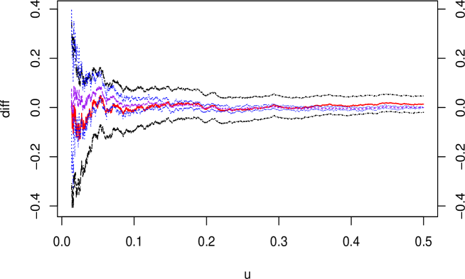
Figure 3 plots the values of $\hat{\alpha}(u)-\alpha(u)$, $\hat{\alpha}^{*}(u)-\alpha(u)$ and their bounds of 90% confidence intervals for a sample of size $n=10000$ from the distribution (12). See also Figure 1(a) for the plot of $\alpha(u)$. For the calculations of $\hat{\alpha}(u)$ and its confidence intervals (9), the sample $\{(x_{1i},x_{2i})\}$ is transformed into the copula sample $\{(u_{1i},u_{2i})\}$ via $u_{ji}=F_{j}(x_{ji})$, where $F_{j}$ is the true margin $(j=1,2)$. The confidence intervals of $\alpha^{*}(u)$ are calculated using the basic bootstrap method based on $999$ resamples of size $10000$; see the last paragraph of Section 5.4 for details. The minimum value of $u$ in the plot is defined as $u_{\rm min}=\min\{u\in(0,0.5];T_{L}(u),T_{U}(u),T_{L}^{*}(u),$ $T_{U}^{*}(u)\geq 30\}\simeq 0.01$ in order that the asymptotic theory is applicable.

The figure suggests that when $u$ is around 0.2 or greater, the performance of both $\hat{\alpha}(u)$ and $\hat{\alpha}^{*}(u)$ seems satisfactory. For $u\leq 0.2$, the difference between the sample analogues and the true value increases with $u$ in general. It appears that the 90% confidence intervals of both $\hat{\alpha}(u)$ and $\hat{\alpha}^{*}(u)$ are generally narrow if $u$ is around 0.2 or more. For $u\leq 0.2$, the smaller the value of $u$, the wider the ranges of the confidence intervals of both $\hat{\alpha}(u)$ and $\hat{\alpha}^{*}(u)$. Interestingly, the confidence intervals of $\hat{\alpha}^{*}(u)$ are narrower than those of $\hat{\alpha}(u)$ in most of the plotted range of $u$. This tendency is particularly obvious in the range $[0.2,0.5]$, where the confidence intervals of $\hat{\alpha}^{*}(u)$ are much narrower than those of $\hat{\alpha}(u)$.

References

- (1)
- Aas et al. (2009) Aas K, Czado C, Frigessi A, Bakken H (2009) Pair-copula constructions of multiple dependence. Insur Math Econ 44(2):182–198.
- (3)
- Czado (2010) Czado C (2010) Pair-copula constructions of multivariate copulas. In Copula Theory and its Applications, Springer, Dordrecht, pp 93–109
- Dehgani et al. (2013) Dehgani A, Dolati A, Úbeda-Flores M (2013) Measures of radial asymmetry for bivariate random vectors. Stat Pap 54:271–286
- Dobrić et al. (2013) Dobrić J, Frahm G, Schmid F (2013) Dependence of stock returns in bull and bear markets. Dependence Model 1:94–110
- Donnelly and Embrechts (2010) Donnelly C, Embrechts P (2010) The devil is in the tails: actuarial mathematics and the subprime mortgage crisis. ASTIN Bulletin 40(1):1–33
- Embrechts et al. (2016) Embrechts P, Hofert M, Wang R (2016) Bernoulli and tail-dependence compatibility. Ann Appl Probab 26(3):1636–1658
- Fermanian et al. (2004) Fermanian JD, Radulovic D, Wegkamp M (2004) Weak convergence of empirical copula processes. Bernoulli 10(5):847–860
- Genest and Nešlehová (2014) Genest C, Nešlehová JG (2014) On tests of radial symmetry for bivariate copulas. Stat Pap 55:1107–1119
- Ghalanos (2020) Ghalanos, A (2020) rugarch: univariate GARCH models, R package version 1.4-2
- Hofert and Koike (2019) Hofert M, Koike T (2019) Compatibility and attainability of matrices of correlation-based measures of concordance. ASTIN Bulletin 49:885–918
- Joe (1997) Joe H (1997) Multivariate models and dependence concepts. Chapman & Hall, London
- Joe (2006) Joe H (2006) Discussion of “copulas: tales and facts” by Thomas Mikosch. Extremes 9(1):37–41
- Joe (2014) Joe H (2014) Dependence modeling with copulas. Chapman & Hall/CRC, Boca Raton, FL
- Joe and Hu (1996) Joe H, Hu T (1996) Multivariate distributions from mixtures of max-infinitely divisible distributions. J Multivar Anal 57:240–265
- Krupskii (2017) Krupskii P (2017) Copula-based measures of reflection and permutation asymmetry and statistical tests. Stat Pap 58:1165–1187
- Krupskii and Joe (2015) Krupskii P, Joe H (2015) Tail-weighted measures of dependence. J Appl Stat 42:614–629
- Lee et al. (2018) Lee D, Joe H, Krupskii P (2018) Tail-weighted dependence measures with limit being the tail dependence coefficient. J Nonparametr Stat 30:262–290
- McNeil et al. (2015) McNeil AJ, Frey R, Embrechts P (2015) Quantitative risk management: concepts, techniques, and tools (revised ed.). Princeton University Press, Princeton, NJ
- Nelsen (2006) Nelsen RB (2006) An introduction to copulas (2nd ed.) Springer, New York
- Nikoloulopoulos et al. (2012) Nikoloulopoulos AK, Joe H, Li H (2012) Vine copulas with asymmetric tail dependence and applications to financial return data. Comput Stat Data Anal 56:3659–3673
- R Core Team (2020) R Core Team (2020) R: a language and environment for statistical computing, R Foundation for Statistical Computing, Vienna, Austria. https://www.R-project.org/
- Rosco and Joe (2013) Rosco JF, Joe H (2013) Measures of tail asymmetry for bivariate copulas. Stat Pap 54:709–726
- Segers (2012) Segers J (2012) Asymptotics of empirical copula processes under non-restrictive smoothness assumptions. Bernoulli 18(3):764–782
- Tsukahara (2005) Tsukahara H (2005) Semiparametric estimation in copula models. Can J Stat 33:357–375
- Yoshiba (2018) Yoshiba T (2018) Maximum likelihood estimation of skew- copulas with its applications to stock returns. J Stat Comput Simul 88(13):2489–2506
Supplementary Material for “Copula-based measures of asymmetry between the lower and upper tail probabilities”
Shogo Kato∗,a, Toshinao Yoshibab,c and Shinto Eguchi a
a Institute of Statistical Mathematics
b Tokyo Metropolitan University
c Bank of Japan
August 4, 2020
The Supplementary Material is organized as follows. Section S1 presents the proofs of Lemma 1 and Theorems 1–5 of the article. Section S2 displays plots of random variates from Clayton copula, Ali-Mikhail-Haq copula and BB7 copula discussed in Sections 4.2 and 6.2 of the article.
S1 Proofs
S1.1 Proof of Theorem 1
S1.2 Proof of Theorem 2
Proof.
If follows from the assumption that there exists a slowly varying function such that as . Similarly, there exists a slowly varying function such that as Therefore
The last equality holds because is slowly varying. If and either or , then
∎
S1.3 Proof of Theorem 3
Proposition 1 implies that can be expressed as
Since , the l’Hôpital’s rule is applicable to the last expression of the equation above. Hence we have
as required. ∎
S1.4 Proof of Lemma 1
It is straightforward to see that and can be calculated as
Noting that , the other expectation and variance, namely, and , can be calculated in a similar manner.
Consider
The first term of the left-hand side of the equation above is
Therefore we have
Similarly, can be calculated. The other covariance can also be obtained via a similar approach, but notice that
The second equality holds because . Thus
S1.5 Proof of Theorem 4
Without loss of generality, assume . Let
Then it follows from Lemma 1 and the central limit theorem that
Define
Applying the delta method, we have
where
The asymptotic variance can be calculated as