CoPlay: Audio-agnostic Cognitive Scaling for Acoustic Sensing
Abstract.
Acoustic sensing manifests great potential in various applications that encompass health monitoring, gesture interface and imaging by leveraging the speakers and microphones on smart devices. However, in ongoing research and development in acoustic sensing, one problem is often overlooked: the same speaker, when used concurrently for sensing and other traditional applications (like playing music), could cause interference in both making it impractical to use in the real world. The strong ultrasonic sensing signals mixed with music would overload the speaker’s mixer. To confront this issue of overloaded signals, current solutions are clipping or down-scaling, both of which affect the music playback quality and also sensing range and accuracy. To address this challenge, we propose CoPlay, a deep learning based optimization algorithm to cognitively adapt the sensing signal. It can 1) maximize the sensing signal magnitude within the available bandwidth left by the concurrent music to optimize sensing range and accuracy and 2) minimize any consequential frequency distortion that can affect music playback. In this work, we design a deep learning model and test it on common types of sensing signals (sine wave or Frequency Modulated Continuous Wave FMCW) as inputs with various agnostic concurrent music and speech. First, we evaluated the model performance to show the quality of the generated signals. Then we conducted field studies of downstream acoustic sensing tasks in the real world. A study with 12 users proved that respiration monitoring and gesture recognition using our adapted signal achieve similar accuracy as no-concurrent-music scenarios, while clipping or down-scaling manifests worse accuracy. A qualitative study also manifests that the music play quality is not degraded, unlike traditional clipping or down-scaling methods.
1. Introduction

Acoustic sensing has been an active field of research in mobile computing community. Typically, an acoustic sensing system leverages the acoustic sensors on commercial-off-the-shell (COTS) smart devices. The system emits inaudible custom ultrasound signals from the speaker and then records the reflections using microphones transforming the device into an active SONAR system that is capable of capturing millimeter-level motion in the environment enabling various applications such as human gesture recognition and tracking (Wang et al., 2022; Koteshwara et al., 2023; Wang et al., 2016; Nandakumar et al., 2016), biosignal monitoring (Nandakumar et al., 2015; Wang et al., 2019; Song et al., 2020). Acoustic sensing offers unique advantages as a novel perception modality: 1) Unlike cameras, it works even in non-line-of-sight or poor light conditions, providing enhanced privacy preservation. 2) The speed of sound is many orders of magnitude slower than the speed of radio frequency (RF), allowing for millimeter-level sensing resolution with a significantly narrower bandwidth. 3) They harness the increasing number of speakers and microphones in IoT devices without necessitating hardware modifications. As such, acoustic sensing is promising in fields like Human-Computer Interaction (HCI) and health monitoring. The research community has been actively working on improving acoustic sensing systems in terms of accuracy, security, etc.
However, one critical issue is often overlooked in ongoing research and developments in acoustic sensing: most systems assume the speaker solely plays the sensing signal. Yet, speakers are conventionally used for speech or music applications. Concurrently using audio applications when emitting sensing signals can cause an overload in the speaker’s mixer. To elaborate, a speaker mixer, or audio mixer, is a software component in the operating systems that mixes audio streams from different applications. To accomplish this, the mixer performs resampling, scaling, and addition to consolidate them into a single stream for output. If the value of the mixed signal exceeds the maximum numerical range supported by the DAC, we call this problem signal overload.
In consequence, the speaker mixer would take two possible actions: one is to clip off the overloaded part; another one is to down-scale the signal to ensure the maximum is within the allowable range, as shown in Fig. 1. Currently, these two strategies are widely adopted by operating systems. In Android, Windows, and Linux, they clip off the exceeding portion; IOS and MacOS scale down all the audio streams by a factor. (Li et al., 2022a; Koteshwara et al., 2023) identified that both these methods will cause degraded quality of music or sensing. 1) Clipping results in distortion in the frequency domain. For example, if the user is playing music or answering a phone call, they will hear buzz sounds. The transmitted sensing signal is also distorted. Since the receiver-side ranging algorithms usually rely on accurate spectrum analysis, such as Fast Fourier Transform (FFT), the clipping will negatively affect the sensing performance. 2) Although down-scaling will not distort the frequency domain, it could significantly decrease the transmitted power of the signal. On the one hand, the volume of the music play goes low thus affecting its usability. On the other hand, down-scaled sensing signals are so weak that they can not propagate far enough in the environment. It is an important factor in the sensing performance as many sensing systems assume that they can use a large volume for the ultrasound to reach a longer detection range.
Beyond identifying the essence of the concurrent music problem in (Li et al., 2022a; Koteshwara et al., 2023), some work tangentially address this using closed-form solutions like echo cancellation (Koteshwara et al., 2023) or interleaving (Nandakumar et al., 2017). But they are limited to certain tasks or hurts the performance. In this work, we aim to propose an algorithmic solution to this problem that outperforms either closed-form methods in prior work or clipping and down-scaling in the current OS.
So, we propose CoPlay, a scaling algorithm, to intelligently adapt sensing signals in consideration of concurrent music applications and maintain optimal sensing and music playback. In specific, it can simultaneously
-
•
maximize the sensing magnitude within the available bandwidth left by the concurrent music to enable optimal sensing performance.
-
•
minimize any consequential frequency distortion.
Nevertheless, achieving these two goals simultaneously is hard because tweaking the signal amplitude in the time domain will cause noisy distortion in the frequency domain. For example, amplitude modulation(AM) will introduce noisy side bands beside the carrier frequency. While, in our case, dynamically scaling amplitude will cause even more frequency distortion and then compromise the sensing.
Therefore, a deep learning algorithm is necessary to dynamically scale the signal, by formalizing these two objectives as an optimization problem. We name it cognitive scaling model, inspired by the concept of cognitive radar (Bell et al., 2015), where the transmission (Tx) signal is adaptively adjusted based on environmental changes. The perception-action cycles of cognition algorithms enable real-time adaptation of the radar. In our paper, we dynamically adjust the Tx ultrasound sensing signal according to the concurrent music. The suggested cognitive scaling algorithm runs in the speaker mixer and aims to diminish the risk of overload distortion while preserving the quality of both sensing and music.
Specifically, the cognitive scaling neural network should work for agnostic music and various types of sensing signals. So, in this work, we examine our model with sine wave and frequency-modulated continuous wave (FMCW) chirp, with different types of concurrent audio, including piano, hot songs, bass, and conversational podcasts. To elaborate, sine and FMCW are the most common signals for acoustic sensing regardless of the receiver-side algorithms. After adapting these signals using CoPlay, the receiver-side algorithm should still work as before, as long as the transmitted signal is barely distorted and is known to the receiver-side algorithms, such as the Doppler effect, time of arrival (ToA), dechirping, etc. More specifically, the sine wave (Koteshwara et al., 2023; Wang et al., 2016; Mao et al., 2019) is simple, narrow-band, but susceptible to interference and noise and has limited range resolution. In contrast, acoustic sensing systems using FMCW chirps (Nandakumar et al., 2015; Zhou et al., 2018; Li et al., 2022b) are better correlated and have flexible range resolution. But it is more complex in frequency spectrum thus more challenging for our model to generate accurately. We had a workshop paper(cop, 2023)(anonymized) presenting preliminary results of only sine waves to embark on prior research conversation. But it couldn’t extend to FMCW signals. In contrast, CoPlay incorporates advanced algorithms with broader experiments, allowing it to process both sine and FMCW.
To mitigate the above challenges, we design a cognitive scaling neural network with WaveNet backbone and custom layers. The model can take multiple types of sensing signal and agnostic concurrent music as input. The output is the cognitively scaled sensing signal. Specifically, we design a custom link function with music as bias, which acts as a filter to normalize the signal within dynamic bandwidth. Besides, we design a kernel to alleviate low-frequency noise stemming from the spectral bias and aliasing in convolution layers(Zhang, 2019; Rahaman et al., 2019). At last, we encode the above optimization goals in the loss terms to maximize the amplitude and minimize the frequency distortion.
To evaluate the model performance beyond numerical loss, we also conduct field studies to show how the adapted signal works in downstream tasks. The study of respiration detection and gesture recognition with 12 users shows that our adapted signals yield the same level of performance as the no-music scenarios. Besides, qualitative study manifests that our algorithms achieve better quality than clipped or down-scaled signals.
To summarize, our work has the following contributions.
-
•
We formalize the problem of concurrent sensing and music as an optimization problem and build a deep-learning-based cognitive scaling algorithm for the mixer, which can enable optimal acoustic sensing performance without affecting the quality of concurrent agnostic music playback.
-
•
We conduct an extensive evaluation of complex types of sensing signals including sine and FMCW and microbenchmark the model performance using various ablation studies and datasets.
-
•
The custom layers in our model offer valuable insights for the special scenario of non-auto-regressive modeling on ultra-high-frequency signals.
-
•
Beyond the analysis of model outputs, we deploy the algorithm in real-world field studies with 12 users. The quantitative and qualitative results show that our algorithm performs well in downstream tasks of respiration detection and gesture recognition, while clipping and downscaling hurt the performance.
In the rest of the paper, first, we detail the related work, problem definition, and model design. Then, we evaluate the model performance with ablation studies, along with quantitative and qualitative field studies. Finally, we address the limitations and future work. Finally, we introduce the related work of acoustic sensing and waveform modeling.
2. Related work
Acknowledging this study as a pilot algorithmic solution to the concurrent music issue in acoustic sensing by framing it as an optimization problem, this section delves into a rundown of this field and associated methodologies. First, we overview the existing acoustic sensing research, noting some studies have offered preliminary investigations of the concurrent music issue, and some tangentially addressed it with closed-form fixes. Secondly, we elaborate on inspirational methods we drew from other fields, including non-autoregressive approaches in audio generation, and anti-aliasing techniques in neural networks for computer vision.
Acoustic sensing: Wireless perception using acoustics is a rising realm for applications such as health monitoring and human-computer interaction. It transforms mobile devices with speakers and microphones into a Sonar system. Typically, the system emits an inaudible ultrasound from the speaker; then the reflections from objects are captured by the microphone and subjected to analysis measuring the Doppler effect(Gupta et al., 2012; Koteshwara et al., 2023), time of flight (ToF) (Li et al., 2022b), direction of arrival (DOA) (Mao et al., 2019; Garg et al., 2021), etc. The signal is usually custom-modulated, such as single-tone sine waves or Frequency-modulated Continuous Wave (FMCW). For example, Amazon Echo (Koteshwara et al., 2023), LLAP (Wang et al., 2016), and (Mao et al., 2019; Fu et al., 2022) uses high-frequency sine waves for presence detection, fingertips tracking, hand tracking and silence speech recognition. Cat (Mao et al., 2016), EchoPrint (Zhou et al., 2018), ApneaApp (Nandakumar et al., 2015) and Lasense (Li et al., 2022b) transmit FMCW signal for localization, face or respiration detection. Besides, synthetic aperture radar (SAR) algorithms are widely used for acoustic imaging, as adapted in (Mao et al., 2018; Wang et al., 2022).
These acoustic sensing research usually focus on improving the sensing accuracy in the absence of concurrent music. However, this problem could cause distortion or lack of power in the received sensing signal. To elaborate, the distortion degrades the receiver-side sensing accuracy because the sensing depends on precise frequency; theoretically, it is a convolution property (when using Fast Fourier Transform (FFT) or correlation), covering methods of the phase-based/frequency-based, DOA and SAR. This underscores the reason behind our incorporation of FFT within the loss function. As for the external background noise, which is more often mentioned in these works, we can easily filter it out with a high-pass filter. However, internal noise—like music playing from the same speaker can bring about different problems, as highlighted in the introduction section.
The concurrent music problem: Covertband (Nandakumar et al., 2017), a human activity detection system using acoustics, first proposed to interleave the concurrent music with the sensing signal; but this method hurts the sample rate exponentially, which degrades both music and sensing, especially ultrasound (17kHz+) that requires at least double sample rate (34kHz) to avoid aliasing. Both (Li et al., 2022a; Koteshwara et al., 2023) underscored that the concurrent music distortion results from mixer overflow and clipping. The experience paper (Li et al., 2022a) validated the performance of their algorithm (Li et al., 2022b) under down-scaling, without proposing new solutions to the problem. But as we discussed above, scaling down causes additional issues. The Google patent (Koteshwara et al., 2023) tried to remove the concurrent music distortions in the spectrum by acoustic echo cancellation (AEC) component, assuming motions are non-symmetric in the spectrum but distortions are. However, this method only applies to simple tasks of sensing such as Doppler-effect-based presence detection. Therefore, in our prior workshop paper(cop, 2023)(anonymized), we attempted to formalize this problem as optimization that is better than down-scaling or clipping. However, this preliminary paper was limited to sine waves but coundn’t extend to FMCW signals. In contrast, CoPlay introduces advanced techniques with broader and larger-scale experiments, enabling it to process both sine and FMCW. The increased complexity in frequency necessitates the utilization of CoPlay’s customized model.
Waveform modeling: Our objective is to address this concern in the mixer for agnostic concurrent audio or operating systems and various downstream sensing tasks. This involves 1) maintaining adequate detection range through a minimal power scaling-down and 2) minimal distortion in frequency. So, we formalize it as an optimization problem and let deep learning act as a window function. This problem is close to waveform modeling in the general audio domain.
Non-autoregressive (non-AR) raw audio generation is an active domain. Their sequence-to-sequence model architecture design for raw waveform has proved effective in many tasks such as including speech synthesis(Oord et al., 2016), sound source separation(Stoller et al., 2018), and music generation(Goel et al., 2022). Standard sequence modeling approaches like CNNs(Oord et al., 2016), RNNs(Mehri et al., 2016), and Transformers(Child et al., 2019) are adapted for waveform modeling. Particularly, WaveNet (Oord et al., 2016) and its variants(Engel et al., 2017; Peng et al., 2020) are fundamental backbone components in such architectures. In this work, we adopt this backbone and show the limitations and comparison of other architectures through experiments.
Our task differs from common waveform modeling, which focuses on audible sound below a few hundred Hz. In contrast, ultrasonic sensing signals are 17kHz+, posing unique challenges due to neural networks’ spectral bias toward learning low-frequency features(Rahaman et al., 2019). Some studies attribute this bias to aliasing, caused by passing the activations through down-sampling layers like convolution and max pooling. Nevertheless, these investigations per spectral bias in neural networks are primarily in computer vision tasks(Zhang, 2019; Michaeli et al., 2023), where their definition of high frequency is much lower than the 17kHz+ ultrasonic waveform. Hence, we draw inspiration from them and customize our own kernels to alleviate this issue in ultrasound modeling particularly.
3. Method
As outlined in Fig. 1, our method is to dynamically scale the sensing signal rather than uniformly down-scaling or clipping. We build a cognitive scaling neural network that can 1) minimal frequency distortion and 2) minimal power down-scaling. This method provides optimal sensing performance and ensures concurrent agnostic audio applications remain unaffected. In this section, we start with interpreting the issue of dynamic scaling, then formalizing our objectives as an optimization problem, with a focus on sine wave and FMCW chirps as representative sensing signals. Following this, we introduce the model structure and its customized layers that we present as a cognitive scaling neural network.
3.1. Understanding the effect of dynamically scaling the signal
Achieving our two objectives simultaneously is hard because just tweaking the signal amplitude in the time domain will cause noisy distortion in the frequency domain. To understand the effect of inordinately tweaking the amplitude, consider amplitude modulation (AM) as an interpretable example. AM is a technique used in telecommunications to transmit information by varying the amplitude of a carrier wave. In Fig. 2, the high-frequency carrier is multiplied by the low-frequency base signal, i.e. amplitude modulated. It causes the frequency spectrum of the signal to spread out with noise. This is because the noisy side bands, located above and below the carrier frequency, are created by the modulation process. In this case, the change is closed-form; the side frequencies are and . (Derivatives can be found in Appendix A). Building upon this observation, our cognitive scaling is namely multiplying the signal with a more complex window function, leading to various sidebands in the frequency. Therefore, this effect of altering signals necessitates the utilization of deep learning in this work; closed-form signal processing methods or traditional machine learning can hardly dynamically control the distortion during generation.

3.2. Sensing signal modulation types
In the field of acoustic sensing, two commonly used types of signals are sine waves and FMCW chirps. These signals serve different purposes and are utilized in various applications within acoustic sensing systems.
Sine waves: A sine wave is a single-frequency oscillation that varies with time according to the mathematical function , where is the amplitude of the sine wave, is the frequency, is the initial phase. They are commonly used in acoustic sensing for tasks such as signal testing, calibration, and as reference signals. They provide a simple and well-defined waveform that is easy to generate and analyze.
FMCW chirps: Frequency Modulated Continuous Wave (FMCW) is a technique where the frequency of a continuous wave changes linearly over time. Basically, they are repeated chirps defined as , where and are the starting and ending frequency of the chip; is the time duration of one chirp. They are widely used in applications like radar and sonar. In acoustic sensing, FMCW signals offer advantages such as improved range resolution and the ability to distinguish between multiple targets. They are particularly useful in applications requiring precise distance measurements and target discrimination.
3.3. Define the problem as optimization
To begin, we establish a formalization of the model input, output, and training objectives in loss function.
Input and output: Let be the sensing signal, i.e. a high-frequency sine or chirp. Concurrently, an App plays music . Then the mixer mixes them within the maximum range of allowed by the number of DAC bits. In this paper, we use signed 16-bit PCM, resulting in a range of . For computation convenience, we set . In general, our goal is to generate a cognitively-scaled sensing signal conditioned on the music ; and the is optimal when satisfying the following objectives defined in the loss.
Loss: The first objective is to maximize the sensing amplitude within the bandwidth left by music. In other words, the amplitude of the mixed signal in time domain should be close to the maximum allowed amplitude . To restate, it is to minimize loss , namely the difference between the magnitude of them. However, this would cause consequential frequency distortion as explained in section 3.1, which deteriorates the receiver-side algorithms since they generally rely on accurate frequency (either FFT convolution or correlation convolution). Therefore, we define another loss as the difference between and in frequency domain; it is the difference between their L-2-norm of FFT coefficients. In summary, our goal is to minimize these two loss terms simultaneously as an optimization problem.
Next, we can further customize the loss for sine and chirps. The L-2 norm of FFT coefficients is then rearranged as
| (1) |
where are the magnitude of the complex number coefficients in FFT, , . And is the target frequency bin containing the ultrasound frequency. is half of the window size since we only take the one symmetric half of the FFT output. The magnitude is normalized by the window size and the maximum allowable amplitude of input , i.e. . The normalization guarantees that the two variable terms in are standardized and unbiased. We call the first half target-loss and the second half recovery-loss. The intention here is to encourage a large value in the target frequency bins, and a close-to-zero value in the others.
Secondly, is the L-2 norm of in time domain normalized by , named as amplitude-loss.
| (2) |
For FMCW chirp, we also want the multiple frequency bins to have even amplitude so that it is well correlated. So, we have an additional variance-loss for FMCW using the standard deviation with zero correction:
| (3) |
Finally, the overall loss equals to the weighted summation of these two terms, where are hyperparameters.
| (4) | ||||
| (5) |
Note that, our loss may not guarantee that falls within []. Therefore, we need to embed this constraint into model layers, as introduced in the following section 3.4 per customized link function.
In practice, we first split the sensing signal and music into small windows and run the optimization for each window. For chirps, the window size should be the size of one chirp. In this paper, we use 18kHz sine wave and 18k-20kHz FMCW signal, with a window size of 512 and a sampling rate of 48kHz. These are common settings and factor in all considerations per efficiency and performance. And our model can be extended to other settings as long as training settings are the same as those in testing.
3.4. Cognitive scaling neural network
Next, we establish a model using a non-AR seq-to-seq network. As depicted in Fig. 3, the inputs are music and sensing and the output is adapted sensing . The model architecture derives from a non-causal WaveNet backbone, followed by an anti-aliasing (sinc) kernel and a custom link function for normalization with agnostic music as bias.

3.4.1. Model architecture with WaveNet backbone
To elaborate, it combines a non-auto-regressive sequence-to-sequence structure with WaveNet backbones. While WaveNet architecture was originally developed for AR modeling, it has since become a basic backbone of various audio models. And we validate this choice in the micro-benchmark section by experimental comparison with sample CNN and RNN backbones. In detail, it employs a stack of dilated convolutional layers which provides better reception fields than conventional ones, making it adept at raw waveform modeling and processing sequential data more efficiently than RNNs. The input of the model is concatenated sensing signal and music of the same length of window size 512. Then the 2-row tensor is passed through 2 layers of Wavenet with fused addition and + multiplication, then dilated convolution (hidden size of 2, kernel size of 5, and dilation rate of 1), and finally residual skip layer (double hidden size except the last layer). Then the outputs pass through conv1d layer to merge the two rows, followed by custom layers to be described in the following sub-sections. Based on observation, we choose a large learning rate of 0.1 with Adam optimizer that is stable in training. For implementation, we refer to the Pytorch code base from DiffSinger (Liu et al., 2022) on HuggingFace.
3.4.2. A sinc kernel for anti-aliasing
At the early stage of experiments, we observe non-negligible low-frequency noise in the model output, especially when modeling FMCW chirps. It is a common problem discussed in the computer vision community that the neural network learns low frequency faster and also down-scaling in layers like convolution and max pooling could induce aliasing.
Therefore, we design a custom sinc kernel for band-passing middle activations to isolate specific frequency bands of interest within the signal. The unique properties of the (sinc) filter, notably its brick-wall characteristic in the frequency domain as its Fourier transform is a rectangular function (Appendix B), makes it a preferred choice of filters over Hamming, etc. So, by putting (sinc) kernel as a layer before the final link function, it mitigates artifacts that may arise in the first stage. For implementation, we use sinc_impulse_response function in the Pytorch experimental nightly version. The negative of it is a high-pass filter. And they can sum to one band-pass filter or more. To demonstrate its effectiveness, we perform ablation in the micro-benchmark section.
Another advantage is its potential to serve as a parameterized kernel when building models for new types of sensing signals other than chirp or sine. A parameterized cutoff could learn a dynamic filter for even multiple signals trained in one model. While we currently train standalone models dedicated to each sensing signal, so that each model achieves optimal performance since we focus on substantiating and validating the underlying concept.
3.4.3. A link function for normalization with agnostic-music as bias
As described, should be within the range of [], namely a normalization with agnostic music as bias. To restate, the output should be where is the activation from the previous layer within [0, 1]. So, to embed this constraint as a trainable layer, we leverage the concept of link function in Generalized Linear Models (GLM); It is in analogy to the logit function for the logistic regression, which uses the prior to target on the probability of binary classification ranging from 0 to 1. Similarly, CoPlay uses a hyperbolic tangent function () as link function that scales the output within [-1, 1]. A bonus is that it encourages the value to approach -1 or 1, which is useful in our cases because we want to maximize the magnitude of the waveform, i.e. close to 1 or -1, as illustrated in Fig. 4. In contrast, clipping simply truncates the output, resulting in loss of information or under-fitting, while is more effective especially when data is continuous and has a wide range of values.
So, we design the layer as follows rather than a min-max clipping: where represents the activations from the previous layer. This scales within . Moreover, during inference, we feed the into the mixer in case exceeds the numerical range. Finally, to quantify the output as integers while the model is trained with float64, our code employs a workaround using the round function: it detaches the difference and then adds it back. Otherwise, the round function or typecast function is not differentiable in PyTorch.

4. Micro-benchmark
In this section, we detail the experiment setup and assess the model performance under various micro-benchmarks, including evaluating the generation across different datasets and music types, as well as at varying levels of music volume. Additionally, ablation studies are conducted to understand the impact of model architecture and multi-task learning weights. Finally, we offer an interpretable analysis of the output’s quality by visualization.
Evaluation metric: In this section, we mainly use loss as the evaluation metric. The detailed definition of loss is in section 3.3. It is the indicator of the relative performance when conducting micro-benchmark experiments. Furthermore, to better interpret the performance, we visualize the output via their frequency spectrums and cross-correlation ranging profiles. Besides, we will further assess the performance in downstream field studies of respiration and gesture detection in the following section. The code will go public on Github upon the acceptance of the paper.
4.1. Datasets
We use four types of concurrent audio to study model’s generalization across agnostic types of music. They are piano music, hot songs, bass music, and speech datasets. Furthermore, for each type, we select two different datasets.
Piano: One dataset is the Beethoven dataset (Mehri et al., 2016), consisting of piano sonatas. It has a total duration of 10 hours and serves as a benchmark music dataset for audio generation. We interpolate the data to a sample rate of 48kHz and cast the 8-bit quantization into a 16-bit signed integer. Another piano dataset is the YouTubeMix dataset (Samplernn., 2017) with higher-quality recordings, with a total duration of 4 hours. And we format it in the same way as the Beethoven dataset.
Hot songs: We select two non-stop playlists of hot songs, featuring top-ranking Billboard songs from 2019 and 2022(YoutubeMix, 2019, 2022), spanning various genres like Pop, Rock, and Hip-hop. Both playlists are around two hours long, sourced from YoutubeMix adhering to the same format.
Bass: To ensure the inclusion of low-frequency audio, we had two bass playlists (YoutubeMix, 2024, 2023a), lasting for one hour and two hours, both of which are downloaded from YoutubeMix under the same data format as above.
Speech: Besides musical audio, we add two conversational speech datasets. They are a mental health podcast featuring Selena Gomez(YoutubeMix, 2023c) and a Conan O’Brien podcast(YoutubeMix, 2023b). Both last over one hour long and are downloaded by YoutubeMix in the same format.
All datasets are then cut into equal-length clips, paired with same-length sensing signal clips as defined in section 3.3.
4.2. Experiment results
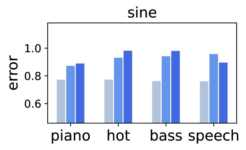


Generalization across datasets and music types: In total, we have 8 datasets, with two datasets for each of the four audio types: piano, hot songs, bass, and speech. When the model is trained and tested with the same dataset, we refer to it as intra-dataset experiment. When training and testing with different datasets from the same type, it is a cross-dataset experiment. Lastly, to assess a more out-of-distribution case, we train on one dataset from one type and test on another dataset from another type, termed as cross-type experiment. Note that, in intra-dataset experiments, we avoid randomly splitting the dataset for testing that is non-realistic in usage. Instead, we take the last 10% of the video as testing set. The rest is then randomly split into 80% training and 20% validation. Fig. 5 shows the average error for an extensive run of these experiments. The results for both sine and chirps are separately plotted as bar charts for different groups of music types. To better plot the error, the y-axis is log-scaled testing loss multiplied by .
In conclusion, the model manifests the capability of generalizing to different types of music or speech, since the cross-dataset error is similar to that of cross-type data error for both sine and FMCW chirps. While intra-dataset usually outperforms the others because the distribution between testing and training is close, the intra-dataset results in chirp are a bit counter-intuitive and it takes 10x more epochs to converge. We think the reason could be that chirp is more complex and needs more data to train, while intra-dataset trains on only 6̃0% of cross-dataset/cross-type experiments. Besides, it is worth mentioning that the cross-type results in the speech group are also good. This is a particularly significant generalization result, since the speech category stands out as the most distinguishable type of audio, compared with music of piano, hot songs, and bass.
| target -loss | recovery -loss | amplitude -loss | variance -loss | |
| sine | 0.5928 | 0.0012 | 0.9558 | - |
| chirp | 0.1852 | 0.0013 | 0.9560 | 0.0214 |
Decompose the loss: The overall error mentioned above comprises multiple loss terms as defined in the section 3.3. Hence, we decompose it into individual loss term values to assess the output per each objective represented by the corresponding loss term. Table. 1 demonstrates the average sub-loss on hot songs datasets. They are training loss including three sub-loss values for sine and an additional variance-loss for FMCW, which we defined above to even the amplitude in the target bandwidth. By default weights, each sub-loss ranges from 0 to 1. We observe that target-loss and amplitude-loss are the bottlenecks, aligning with the intuition that minimizing frequency distortion and maximizing the amplitude are opposed objectives, which is a common issue in multi-task learning. This table serves as a reference for tweaking the weights of loss terms to specific downstream task requirements. For instance, near-field sensing tasks can sacrifice amplitude for minimal distortion.
Varying music volume: Although it is possible that a high volume of music might degrade our model performance, Fig. 6(b) shows that the overall error does not increase with music volume. In detail, we train with the same sub-loss experiment and test with increasing levels of music volume. The x-axis indicates the ratio of sensing signal volume and music volume. The default ratio is 1:1, and 0.6:1.4 is when music is roughly double in power, equivalently 7.3db louder. In summary, CoPlay is stable when training with agnostic music even in unseen volume. This could be attributed to the normalization in the definition of our amplitude-loss and recovery-loss.
Ablation of model architecture: In terms of the model design, we justify our choice by comparing the model performance under different model backbones. We considered three models namely CNN, RNN, and Wavenet with the same number of recursive layers. Fig. 6(a) shows that Wavenet slightly outperforms CNN and both surpass RNN. But CNN has a limited reception field so we chose Wavenet which is better at overcoming this issue with dilated convolution layers. Furthermore, the sample RNN uses LSTM layers which is less efficient to train in comparison.
Ablation of multi-task loss terms: The overall loss consists of sub-loss terms, each of which represents different objectives of optimization (section 3.3). By default, they are assigned equal weights. So, we ablate the weights to assess the performance when we emphasize on certain objective. In detail, recovery-loss is set to one by default, the same as other sub-losses. Hence, we also run the same ablation setup but increase the weight of recovery-loss from 1 to 1.2, 1.4, and 1.6, making it the largest sub-loss, i.e. making minimizing frequency distortion the most significant objective; this is a practical use case when certain sensing systems, like near-field tasks, can compromise the power for minimal frequency distortion. In Fig. 6(c), the error roughly goes down with the increase in weight, which serves as a reference for tuning this ratio for the downstream tasks in practice.
Ablation of sinc filter: Finally, we conduct an ablation to evaluate the effectiveness of the sinc filter as defined in section 3.3. It’s also the same experiment set up as the above ablation study. As shown in Fig. 6(d), both the sine and chirp models exhibit improved performance with the presence of sinc kernel, especially the sine wave model. We attribute this enhancement to the narrow target main lobe in the spectrum of sine, thus more side lobes are to be suppressed. The sinc kernel helps significantly reduce these lobes, resulting in a lower numerical loss. In summary, this ablation study validates the efficacy of the sinc filter, and we incorporate this essential layer in all of our experiments.
4.3. Spectral analysis
Training procedure in 3D frequency domain: Although the numerical loss can indicate the model performance, we seek a more comprehensive perspective by visualizing the model output in frequency spectrum. This helps confirm that the output aligns well with expectations. In Fig. 7, we take the FFT of a sample window output and screenshot it with the increasing training epochs. The rise of the yellow peaks indicates that it converges to an 18kHz sine wave or 18k-20kHz FMCW as the training epoch increases. The side lobes are much weaker than the main lobes, which manifest good SNR. (Moreover, we further substantiate the SNR by qualitative study in section 5)


Ranging profile with cross-correlation: Likewise, certain sensing algorithms employ cross-correlation (Xcorr) to obtain the ranging profile instead of utilizing FFT. Nevertheless, they basically use equivalent computation components: convolution or even DFT. For instance, an accelerated computation of Xcorr is to perform a frequency-domain Xcorr, which is faster than that in the time domain (Dr. Erol Kalkan, 2023), because shifting a signal in the time domain is equivalently scaling it in the frequency domain. Therefore, in addition to plotting the FFT spectrums of the generated signal, Fig. 8 shows the Xcorr correlation output for the cognitively-scaled signal. By rolling the signal in the time domain, the distinct peak in Xcorr output changes with the number of shifts as expected. In summary, this justifies that our adapted signal works well even if the receiver-side sensing algorithm uses Xcorr.

4.4. Computation efficiency
We refer to CoPlay as a mixer algorithm, by expecting that our cognitive scaling can be applied to the buffered audio stream in the speaker. So, we run training and inference on small windows of audio clips. In this paper, we test with window size of 512, which is a common setting for acoustic sensing and also meets the computation efficiency requirement. To elaborate on the computation cost, our model has a size of 5.5 KB, forward/backward pass size of 0.98 MB, and an input size of 0.07 MB. The estimated total size of training is 1.05 MB only, which indicates the inference could easily fit into the RAM of commercial smartphones or other mobile devices. Despite that it was trained on an RTX 8000 GPU, it can run inference for roughly 625 fps on mobile devices, equivalently per frame. On the other hand, the buffer interval is roughly , which leaves quite enough time for inference on one frame. Therefore, it can run in real time with no perceptible delay. Furthermore, the entire audio is actually pre-known by the speaker in many cases. For instance, Java sound API can load the audio file into memory and then buffer the sliding windows into input stream. That’s saying, the speaker can run the inference upfront and before playing the processed signal. Moreover, there is a lot of literature on model compression and inference acceleration to further improve the efficiency, which is beyond the scope of this work.
We also plot the roofline in Fig. 9, illustrating our model on RTX 3080 GPU in comparison with other popular models; ours is much more memory-efficient than even the mobile models like MobileNet, SqueezeNet, and DenseNet, because of its small number of parameters of dilated layers. We also show dashed rooflines from other popular mobile SoCs(System-on-a-Chip) and GPUs as a comparison of their peak performance and max memory bandwidth, which validates that our model would work on most chips, especially mobile chips like Snapdragon 888 and Kirin 9000.

5. field study: respiration rate detection and hand gesture recognition
To better evaluate our method in practice beyond the micro-benchmark, we run our algorithm in two downstream acoustic sensing tasks: respiration rate detection and hand gesture recognition. These field studies demonstrate the power of CoPlay for improving the performance of various downstream tasks when there is interference from concurrent audio applications. The field studies are chosen to be controlled, to ablate-study the effects of our method, avoiding uncontrolled results from other factors like occlusion or range.
In summary, we run these 2 tasks with 2 types of sensing signals and 3 types of audio (piano, hot songs, and podcast) on 2 types of devices with 12 users in comparison with 4 baselines. In this section, we detail the tasks, evaluation metrics, hardware/software setups, and study design. Then we compare with 4 baselines of clipping, down-scaling, and no-music. The quantitative and qualitative results show that our method matches the sensing performance that has no music interference, while we have no issues as clipping and down-scaling have.
5.1. Tasks and evaluation metrics
In the field study, we evaluate our cognitive scaling mixer algorithm in two tasks: respiration rate detection and hand gesture recognition. In each task, we play inaudible ultrasound (sine or FMCW) from a mobile phone (IOS or Android) and then analyze received signals for recognition.
Respiration monitoring is a well-explored application in acoustic sensing, manifesting its high resolution that can detect subtle millimeter-level motions. The target is to get breath per minute BPM by detecting peaks in the waveform of chest movement during inhalations. Therefore, in the following results, we show the mean absolute error MAE of BPM and visualize chest movement in a waveform.
Hand gesture recognition is another important use case showing that acoustic sensing can leverage patterns in received signals for profound motion recognition. In this study, we classify three gestures: swipe, push, and pinch, which are essential in commercial gesture control systems. In the following result section, we show the classification accuracy and the confusion matrix as well.
5.2. Experiment setup
Hardware: We run acoustic sensing on two mobile phones: a Samsung smartphone and an iPhone, representing the mobile operation systems of Android and IOS, because their built-in algorithm handling overflow in the speaker mixer is different. As discussed above, Android turns to clip, IOS turns to scale down. Both phones are placed on the desk around 40cm away from the seated user facing the phone; one phone at a time.
The ground truth for respiration detection is from the Go Direct Respiration Belt, a belt with a force sensor (Belt, 2023). The user wears it around the chest or abdomen. It also has a built-in breath rate calculation every 10 seconds. The sample window for the calculation is 30 seconds. To get the ground truth label for gesture recognition, we play a guiding video on a monitor and ask the user to follow the video to conduct specific gestures at a guided time every 3 seconds.
Data collection software: We developed our own data collection App for both Android and IOS. The recorder operates at a sample rate of 48k HZ. The recording format is 16-bit PCM. Both the transmitter and receiver are set to use the mono channel. And the volume of concurrent music is around 50db-60db. These are commonly supported audio parameters in mobile phones.
There is also a data collection program running on a laptop for synchronous ground truth data recording using the respiration monitoring belt. It calls the Python SDK of GoDirect (Belt, 2023) and runs as a Flask Restful API on a Macbook. The API is invoked by the data collection mobile App to start the recording of sensing and ground truth synchronously. The hand gesture guiding video also runs an API on the laptop to start playing the video synchronously.
Sensing algorithm: As for the receiver side sensing algorithm, we select two classic ones for the sine and FMCW signal separately. Note that we aim to show the effectiveness of CoPlay from the perspective of downstream task accuracy here, while many other factors could affect the accuracy, including the receiver-side sensing algorithm. So, the two selective ones are a baseline to show the relative effectiveness of our CoPlay V.S. baselines; Improving the receiver-side sensing algorithm is not the focus of this study.
As discussed above, almost all receiver-side algorithms are based on the Fourier transform in some way. Therefore, for the respiration rate detection, we play a sine wave signal at 18kHz and extract that frequency bin in the received signal, whose amplitude is proportional to the chest-to-device distance. Next, we apply peak detection on the amplitude waveform to get BPM. We use the basic Scipy peak detection function with default parameters; it finds all local maxima by simple comparison of neighboring values. Besides, to eliminate noisy motion other than the breath -for example, body or head rotation- we apply a band-pass filter before peak detection. The filter selects out 8-22Hz because the human breath rate is typically 12-18Hz. Specifically, we use the same window size of 30s and interval of 10s as the Vernier belt ground truth. The beginning ¡30s are padded.
For the gesture recognition task, we transmit FMCW of 18k-20kHz and then dechirp the received signal with cross-correlation to get a range profile. At last, each window subtracts its previous window to eliminate the static environment and let the motions stand out. Note that nearby motions other than the hand would degrade sensing performance. So, we ask the users to try their best to stay still, since robustness under noise is not the focus of this study; we control these conditions to isolate the effectiveness of CoPlay only. Finally, the range profile is input into a simple CNN classifier (Document, 2023) as a single-channel 2D feature map. The CNN is a simple 2-conv-layer network with max pooling, ReLU, plus three linear layers at the end. Then by training with Adam optimizer and cross-entropy loss, we got a 3-class classifier. Besides, to avoid overfitting on our small dataset, we augment the feature map by adding Gaussian noise in the training dataloader. This regulation helps the training loss converge fast and stable. The classifier is trained in a leave-one-user-out manner and the following results are the average accuracy.
5.3. Study procedure
In the study, we first brief the participants on our IRB and study procedure without telling them the order and content of the audio to be played. Then we conduct 2 sessions of data collection; each has 6 sub-sessions. Upon finishing each sub-session, we ask the user to fill in a qualitative questionnaire about the music quality they heard. In total, each user collects 12 minutes of data and we have around 2 hours total data from 12 users.
For each user, the 2 sessions of data collection cover the two tasks of respiration and gesture detection separately. Within each session, there are 6 sub-sessions that are 6 minutes in total. The first three sessions run on the Android phone, playing 1) sensing signal only, no-music 2) audio + cognitively-scaled sensing 3) audio + sensing (cause clipping). The other three sessions run on the iPhone, playing the same audio except that the third case will cause down-scaling instead. Sub-session 1 and 3 are baselines to compare with our method in sub-session 2. Sub-sessions 2 and 3 use the same audio clip, which consists of samples from the datasets we used in the micro-benchmark section. It concatenates three 20-second clips from each of the three types of audio, including piano, hot songs, and speech. At the beginning of the first session, the user starts by putting on the belt and sitting in front of the device. Then they click the button on the phone screen to start recording. In between the sub-sessions, we switch the phone. Next, for the second session, they can take off the belt. Likewise, they will also click the button to start recording and playing the guiding video. Upon finishing every 3 sub-sessions, the user fills in the qualitative questionnaire about music quality and volume.
5.4. Study results with baselines
5.4.1. CoPlay V.S. Baselines (clipping and down-scaling)
First, we compare CoPlay with the baselines. They are no-music baseline, clip baseline, and two downscale baselines, measuring both the error of BPM and the accuracy of gesture recognition. As depicted in Fig. 10, our cognitively-scaled sensing with concurrent music achieves similar results as the sensing-with-no-music baseline; while the other three baselines exhibit inferior performance compared to the no-music. These results are an average of experiments across all devices, users, and audio types. Specifically, in the two downscale experiments, we reduce the power of sensing by half and leave the rest half for music. Additionally, the down_x2 refers to further scaling down the sensing signal to 1/4 of the original, resulting in a decrease of 12db in volume (sound pressure level is ), then the music takes 3/4. Note that it is equivalent to double the sensing distance, as signal intensity is inversely proportional to the square of the distance from the source. In summary, both clipping and downscaling underperform our algorithm. Clipping emerges as the worst, even than large scaling down; while downscaling would get worse quadratically with increasing distance in practice, although the drop is less noticeable when compared with the worst case from clipping in our experiment. In the subsequent section, we will elucidate these observations by visually analyzing their breakdowns.


5.4.2. Visualization and error analysis

Fig. 11 depicts the amplitude of detected breath rhythm of the three scenarios: no-music, CoPlay, and clip(Android) or downscale (IOS). To recap, the amplitude of breath rhythm is the normalized amplitude of FFT at 18k, named , which is roughly proportional to the chest-to-device distance. First, it is obvious that the no-music scenario for both Android and IOS is stronger than our cognitively scaled signal. While clipping also keeps the received amplitude strong, it is significantly noisy because it is distorted by the mixer at the transmitter. Relatively, CoPlay and no-music scenarios are clear periodic waveforms. Secondly, the downscale case is almost two times weaker than the no-music case, while CoPlay is only 15% weaker. Besides, its crests and troughs are not as observable as the others, which is ineffective for peak detection. The ground truth BPM of the two selected samples are a) 18.5 and b) 18.9. As shown in the legend in the figures, CoPlay and the no-music baseline are close to the ground truth BPM while clip and downscale have a larger error. The dots along each line are the individual breath selected by the peak detection algorithm.
In Fig. 12, to take a closer look at the visualization of our output, we zoom in on the first line plot of CoPlay and plot it with the normalized ground truth in the background. The dashed line is the force sensor recording, from which the Vernier Belt derives the BPM. The peaks align well even though the overall amplitude rises and falls, which substantiates the effectiveness of CoPlay.

Furthermore, we take a closer look at the errors of gesture classification by calculating the confusion matrix that plots accuracy for each class. Since our method and no-music baseline are 100% accurate, Fig. 13 lists the confusion matrix of the downscale baseline and the clip baseline. As expected, wireless sensing is more sensitive to vertical motion, i.e. pushing close to or away from the device, because the distance of reflection traveling in the air changes dramatically. So, the errors are high in the swipe and pinch rows/columns in the confusion matrix, while push is almost always recognized accurately.


5.4.3. Qualitative study
Table. 2 is the result of the qualitative study. They are the playback quality of each sub-session per level of buzzing noise, loudness, and delays. The scores are the average of all users’ answers, asking for a 1 - 5 scale (integer) per question:
-
•
Q.1. Did you hear a buzzing noise?
-
•
Q.2. Did you hear the music at adequate volume?
-
•
Q.3. Did you perceive delay or discontinuity?
The score of Q.1 justifies that clipping does cause audible noise, basically buzzing, while CoPlay and down-scaling do not. Q.2 manifests that down-scaling hurts the power of audio signals, resulting in the users being unable to hear the audio at a sufficient volume. To elaborate, in the study, we calibrated the system volume of the phone to 50db, a common loudness of music playback or a nearby conversational talk. The volume was measured by another smartphone App placed next to the study device. When down-scaling happens, the music volume reduces by 6db per each half down-scaling. Q.3 is to prove that the computation overhead of CoPlay does not cause any discontinuity or delay between the chunks of processed clips.
| clipping | downscale | CoPlay | |
| Q.1 (5 = buzzing) | 4.72 | 1.13 | 1.22 |
| Q.2 (5 = loud) | 4.14 | 1.12 | 4.49 |
| Q.3 (5 = delay) | - | - | 1 |
6. discussion and future work
In this work, our system handles two types of sensing signals on two downstream applications. In the future, in order to explore the full extent of applicable scenarios and thoroughly assess the versatility of the proposed approach, it would be prudent to engage in a more expansive array of field studies and sensing signals. These studies could extend beyond the initial scope of simple tasks and delve into more intricate downstream tasks such as more fine-grained gesture recognition. Specifically, evaluating the algorithm’s performance in challenging environments, characterized by varying degrees of interference (like motion, external noise, etc), could yield valuable insights into its robustness and effectiveness under diverse conditions.
Moreover, we recognize a potential escalation in computational costs, particularly when dealing with multiple channels. Presently, our assumptions are based on the notion that devices with multiple channels duplicate the same signal into each channel. However, in the realm of 3D spatial audio applications, there exists the possibility of having slightly different signals per channel. Although our algorithm remains non-intrusive to the music itself, the need for custom cognitive scaling for each channel introduces an increase in computational demands. It would be worthy to delve deep into evaluating the computation cost of our algorithm in these more realistic scenarios and apply state-of-the-art acceleration methods from the perspectives of both the model compression and on-device streaming data processing.
Furthermore, we aim to delve deeper into investigating the behavior of speaker mixers through the execution of real-world experiments across a more diverse range of devices. This expanded investigation seeks to provide a more comprehensive understanding of how speaker mixers function in various technological contexts. Besides, the variant of the number of sensors and their positions are also relevant factors remained to be investigated. For example, smart speakers like Amazon Echo Dot and Google Home have much more powerful speakers and the full stack runs on unique IoT operating systems, the combination of which could bring distinct insights to the scope of our concurrent music problem.
References
- (1)
- cop (2023) 2023. Anonymized workshop paper.
- Bell et al. (2015) Kristine L Bell, Christopher J Baker, Graeme E Smith, Joel T Johnson, and Muralidhar Rangaswamy. 2015. Cognitive radar framework for target detection and tracking. IEEE Journal of Selected Topics in Signal Processing 9, 8 (2015), 1427–1439.
- Belt (2023) Go Direct Vernier Belt. 2023. Go Direct Python SDK. https://github.com/VernierST/godirect-examples/tree/main/python
- Child et al. (2019) Rewon Child, Scott Gray, Alec Radford, and Ilya Sutskever. 2019. Generating long sequences with sparse transformers. arXiv preprint arXiv:1904.10509 (2019).
- Document (2023) Pytorch Document. 2023. Training a classifier - cifar10 tutorial. https://pytorch.org/tutorials/beginner/blitz/cifar10_tutorial.html#define-a-convolutional-neural-network
- Dr. Erol Kalkan (2023) P.E. Dr. Erol Kalkan. 2023. xcorrFD(x,y) MATLAB Central File Exchange. (January 27 2023). https://www.mathworks.com/matlabcentral/fileexchange/63353-xcorrfd-x-y
- Engel et al. (2017) Jesse Engel, Cinjon Resnick, Adam Roberts, Sander Dieleman, Mohammad Norouzi, Douglas Eck, and Karen Simonyan. 2017. Neural audio synthesis of musical notes with wavenet autoencoders. In International Conference on Machine Learning. PMLR, 1068–1077.
- Fu et al. (2022) Yongjian Fu, Shuning Wang, Linghui Zhong, Lili Chen, Ju Ren, and Yaoxue Zhang. 2022. SVoice: Enabling Voice Communication in Silence via Acoustic Sensing on Commodity Devices. In Proceedings of the 20th ACM Conference on Embedded Networked Sensor Systems. 622–636.
- Garg et al. (2021) Nakul Garg, Yang Bai, and Nirupam Roy. 2021. Owlet: Enabling spatial information in ubiquitous acoustic devices. In Proceedings of the 19th Annual International Conference on Mobile Systems, Applications, and Services. 255–268.
- Goel et al. (2022) Karan Goel, Albert Gu, Chris Donahue, and Christopher Ré. 2022. It’s raw! audio generation with state-space models. In International Conference on Machine Learning. PMLR, 7616–7633.
- Gupta et al. (2012) Sidhant Gupta, Daniel Morris, Shwetak Patel, and Desney Tan. 2012. Soundwave: using the doppler effect to sense gestures. In Proceedings of the SIGCHI Conference on Human Factors in Computing Systems. 1911–1914.
- Koteshwara et al. (2023) Krishna Kamath Koteshwara, Zhen Sun, Spencer Russell, Tarun Pruthi, Yuzhou Liu, and Wan-Chieh Pai. 2023. Presence detection using ultrasonic signals with concurrent audio playback. US Patent 11,564,036.
- Li et al. (2022a) Dong Li, Shirui Cao, Sunghoon Ivan Lee, and Jie Xiong. 2022a. Experience: practical problems for acoustic sensing. In Proceedings of the 28th Annual International Conference on Mobile Computing And Networking. 381–390.
- Li et al. (2022b) Dong Li, Jialin Liu, Sunghoon Ivan Lee, and Jie Xiong. 2022b. Lasense: Pushing the limits of fine-grained activity sensing using acoustic signals. Proceedings of the ACM on Interactive, Mobile, Wearable and Ubiquitous Technologies 6, 1 (2022), 1–27.
- Liu et al. (2022) Jinglin Liu, Chengxi Li, Yi Ren, Feiyang Chen, and Zhou Zhao. 2022. Diffsinger: Singing voice synthesis via shallow diffusion mechanism. In Proceedings of the AAAI conference on artificial intelligence, Vol. 36. 11020–11028.
- Mao et al. (2016) Wenguang Mao, Jian He, and Lili Qiu. 2016. Cat: high-precision acoustic motion tracking. In Proceedings of the 22nd Annual International Conference on Mobile Computing and Networking. 69–81.
- Mao et al. (2018) Wenguang Mao, Mei Wang, and Lili Qiu. 2018. Aim: Acoustic imaging on a mobile. In Proceedings of the 16th Annual International Conference on Mobile Systems, Applications, and Services. 468–481.
- Mao et al. (2019) Wenguang Mao, Mei Wang, Wei Sun, Lili Qiu, Swadhin Pradhan, and Yi-Chao Chen. 2019. Rnn-based room scale hand motion tracking. In The 25th Annual International Conference on Mobile Computing and Networking. 1–16.
- Mehri et al. (2016) Soroush Mehri, Kundan Kumar, Ishaan Gulrajani, Rithesh Kumar, Shubham Jain, Jose Sotelo, Aaron Courville, and Yoshua Bengio. 2016. SampleRNN: An unconditional end-to-end neural audio generation model. arXiv preprint arXiv:1612.07837 (2016).
- Michaeli et al. (2023) Hagay Michaeli, Tomer Michaeli, and Daniel Soudry. 2023. Alias-Free Convnets: Fractional Shift Invariance via Polynomial Activations. In Proceedings of the IEEE/CVF Conference on Computer Vision and Pattern Recognition. 16333–16342.
- Nandakumar et al. (2015) Rajalakshmi Nandakumar, Shyamnath Gollakota, and Nathaniel Watson. 2015. Contactless sleep apnea detection on smartphones. In Proceedings of the 13th annual international conference on mobile systems, applications, and services. 45–57.
- Nandakumar et al. (2016) Rajalakshmi Nandakumar, Vikram Iyer, Desney Tan, and Shyamnath Gollakota. 2016. Fingerio: Using active sonar for fine-grained finger tracking. In Proceedings of the 2016 CHI Conference on Human Factors in Computing Systems. 1515–1525.
- Nandakumar et al. (2017) Rajalakshmi Nandakumar, Alex Takakuwa, Tadayoshi Kohno, and Shyamnath Gollakota. 2017. Covertband: Activity information leakage using music. Proceedings of the ACM on Interactive, Mobile, Wearable and Ubiquitous Technologies 1, 3 (2017), 1–24.
- Oord et al. (2016) Aaron van den Oord, Sander Dieleman, Heiga Zen, Karen Simonyan, Oriol Vinyals, Alex Graves, Nal Kalchbrenner, Andrew Senior, and Koray Kavukcuoglu. 2016. Wavenet: A generative model for raw audio. arXiv preprint arXiv:1609.03499 (2016).
- Peng et al. (2020) Kainan Peng, Wei Ping, Zhao Song, and Kexin Zhao. 2020. Non-autoregressive neural text-to-speech. In International conference on machine learning. PMLR, 7586–7598.
- Rahaman et al. (2019) Nasim Rahaman, Aristide Baratin, Devansh Arpit, Felix Draxler, Min Lin, Fred Hamprecht, Yoshua Bengio, and Aaron Courville. 2019. On the spectral bias of neural networks. In International Conference on Machine Learning. PMLR, 5301–5310.
- Samplernn. (2017) DeepSound. Samplernn. 2017. Samplernn. https://github.com/deepsound-project/samplernn-pytorch
- Song et al. (2020) Xingzhe Song, Boyuan Yang, Ge Yang, Ruirong Chen, Erick Forno, Wei Chen, and Wei Gao. 2020. SpiroSonic: monitoring human lung function via acoustic sensing on commodity smartphones. In Proceedings of the 26th Annual International Conference on Mobile Computing and Networking. 1–14.
- Stoller et al. (2018) Daniel Stoller, Sebastian Ewert, and Simon Dixon. 2018. Wave-u-net: A multi-scale neural network for end-to-end audio source separation. arXiv preprint arXiv:1806.03185 (2018).
- Wang et al. (2019) Anran Wang, Jacob E Sunshine, and Shyamnath Gollakota. 2019. Contactless infant monitoring using white noise. In The 25th Annual International Conference on Mobile Computing and Networking. 1–16.
- Wang et al. (2022) Penghao Wang, Ruobing Jiang, and Chao Liu. 2022. Amaging: Acoustic Hand Imaging for Self-adaptive Gesture Recognition. In IEEE INFOCOM 2022 - IEEE Conference on Computer Communications. 80–89. https://doi.org/10.1109/INFOCOM48880.2022.9796906
- Wang et al. (2016) Wei Wang, Alex X Liu, and Ke Sun. 2016. Device-free gesture tracking using acoustic signals. In Proceedings of the 22nd Annual International Conference on Mobile Computing and Networking. 82–94.
- Wikipedia (2023) Wikipedia. 2023. Amplitude modulation. https://en.wikipedia.org/wiki/Amplitude_modulation
- YoutubeMix (2019) YoutubeMix. 2019. Pop music 2019 dataset. https://www.youtube.com/watch?v=-hg7ILmqadg
- YoutubeMix (2022) YoutubeMix. 2022. Pop music 2022 dataset. https://www.youtube.com/watch?v=v8ASOBDTifo
- YoutubeMix (2023a) YoutubeMix. 2023a. Bass guitar lo-fi mix dataset. https://www.youtube.com/watch?v=UET4X_UgF5k
- YoutubeMix (2023b) YoutubeMix. 2023b. Podcast by Conan O Brien dataset. https://www.youtube.com/watch?v=du2sCHXJf2A
- YoutubeMix (2023c) YoutubeMix. 2023c. Podcast by Selena Gomez dataset. https://www.youtube.com/watch?v=AmARvccsdMI
- YoutubeMix (2024) YoutubeMix. 2024. Bass boosted music mix dataset. https://www.youtube.com/watch?v=RULRXAf5AC8
- Zhang (2019) Richard Zhang. 2019. Making convolutional networks shift-invariant again. In International conference on machine learning. PMLR, 7324–7334.
- Zhou et al. (2018) Bing Zhou, Jay Lohokare, Ruipeng Gao, and Fan Ye. 2018. EchoPrint: Two-factor authentication using acoustics and vision on smartphones. In Proceedings of the 24th Annual International Conference on Mobile Computing and Networking. 321–336.
Appendix A An example of inordinate amplitude modulation and consequential frequency distortion.
Amplitude modulation (AM) is a modulation technique where the amplitude of a carrier signal is varied in proportion to the instantaneous amplitude of a modulating signal. Here is a simple case and the formulas of how the side frequencies derivative(Wikipedia, 2023).
The carrier signal is denoted as
And the modulating signal is
The amplitude modulation (AM) signal results when carrier is multiplied by the positive quantity of the modulating signal:
| (6) | ||||
| (7) | ||||
| (8) |
By rearranging
| (9) | ||||
| (10) | ||||
| (11) |
Finally,
| (12) | ||||
| (13) | ||||
| (14) |
where . By deriving , it becomes a modulated signal with two additional frequencies and besides the original . The three components are called the carrier, the upper sideband (USB), and those below the carrier frequency constitute the lower sideband (LSB). This is an explicit example of how inordinate changes in time domain amplitude result in side lobes in frequency distortion. Which guides the problem definition in this paper.
Appendix B Sinc function as a brick-wall filter.
If we need a filter that yields minimal artifacts, its frequency response needs to be a rectangular function, namely a brick-wall filter:
Where is the bandwidth, i.e. the cutoff frequency. Then its impulse response is given by the inverse Fourier transform of its frequency response:
| (15) |
Let , then
| (16) | ||||
| (17) | ||||
| (18) | ||||
| (19) | ||||
| (20) |
It turns out to be a function with cutoff . Furthermore, windowed-sinc finite impulse response is an approximation of sinc filter. It is obtained by first evaluating sinc function for given cutoff frequencies, then truncating the filter skirt, and applying a window, such as the Hamming window, to reduce the artifacts introduced from the truncation.