Cooperative Transportation with Multiple Aerial Robots and Decentralized Control for Unknown Payloads

Koshi Oishi¹, Yasushi Amano¹, and Tomohiko Jimbo² ¹The authors are with the Cloud Informatics Research-Domain, Toyota Central R&D Labs., Inc., 41-1, Yokomichi, Nagakute, Aichi, Japan [email protected]²The author R-Frontier Division, Frontier Research Center. Toyota Motor Corporation, 1, Toyota-cho, Toyota, Japan

Abstract

Cooperative transportation by multiple aerial robots has the potential to support various payloads and to reduce the chance of them being dropped. Furthermore, autonomously controlled robots make the system scalable with respect to the payload. In this study, a cooperative transportation system was developed using rigidly attached aerial robots, and a decentralized controller was proposed to guarantee asymptotic stability of the tracking error for unknown strictly positive real systems. A feedback controller was used to transform unstable systems into strictly positive real ones using the shared attachment positions. First, the cooperative transportation of unknown payloads with different shapes larger than the carrier robots was investigated through numerical simulations. Second, cooperative transportation of an unknown payload (with a weight of about $2.7$ kg and maximum length of $1.6$ m) was demonstrated using eight robots, even under robot failure. Finally, it was shown that the proposed system carried an unknown payload, even if the attachment positions were not shared, that is, even if the asymptotic stability was not strictly guaranteed.

I INTRODUCTION

Recently, aerial robots have been used in various fields such as photography, agriculture, and transportation[1, 2, 3]. These robots can move in three dimensions, so they do not depend on the construction of ground infrastructure, and transportation by aerial robots can be used to provide a wide range of services [4]. However, the payload that can be transported by a single aerial robot is a major limiting factor, and if an aerial robot fails, it cannot be controlled. The limitation can be overcome by implementing a cooperative transportation system using multiple aerial robots. This system is expected to relax payload limitations, including shape and mass, and reduce the chance of a load being dropped. Furthermore, if each robot operates autonomously, the plugin/out of robots can be performed easily, and the expandability of the system will be improved.

Cooperative transportation by multiple aerial robots has been widely reported[5, 6], and the system configurations may be divided into two main categories: cable-suspended [7, 8, 9, 10, 11, 12] and rigidly connected[13, 14, 15, 16]. Wehbeh et al. [12] also proposed a system using rigid rods and ball joints, which is similar to cable-suspended configurations. Studies of cable-suspended configurations have mainly focused on robot formations [9] and leader tracking [10, 11]. Gassner et al. [10] proposed a decentralized control system where one follower detects the leader with a camera, and they verified the method using two aerial robots.

In contrast, rigidly connected configurations are simpler than cable-suspended configurations, and the aerial robots have less risk of colliding. However, because the robots hold a payload directly, the rigidly connected configurations are more difficult to coordinate than cable-suspended ones [13]. Mellinger et al. [13] proposed a decentralized controller, and they demonstrated it with aerial robots and a lightweight payload. In addition, Wang et al. [16] proposed a decentralized controller limited to centrosymmetric formations. The effectiveness of this approach was confirmed by simulation, but not by actual robots. Owing to the constraints of rigidly connected configurations, few experiments have been conducted with actual robots.

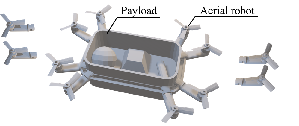
Refer to caption — (a) Rigidly connected robots to a payload

In our previous study [17], we used robots that were able to communicate with each other to estimate the mass and the position of the center of mass (COM) and share the derived mixed matrix, which could be used for stabilization during transportation. In contrast, this study investigates decentralized control for a cooperative transportation system with rigid connections, as shown in Fig. 1. The proposed method does not use a mixed matrix or require communication to estimate the COM. Instead, by sharing the attachment point, each robot derives a controller that is robust to the fluctuations of the payload (mass and COM) and robot failures to achieve stabilization. From a practical perspective, it is desirable to prove the asymptotic stability of the controller relative to a reference. Therefore, we extend the autonomous smooth switching controller (ASSC) [18], whose asymptotic stability has been proven for single-output systems, to multiple-output systems. However, aerial transportation systems are unstable and ASSC is only applicable to strictly positive real (SPR) systems. Therefore, we introduce a feedback controller that transforms the system into an SPR system by sharing the attachment positions among the robots. The contributions of this study are as follows:

•

A novel decentralized controller based ASSC is proposed for unstable transportation systems. This proposed controller is robust against expected fluctuations (mass, COM, and failures) and the asymptotic stability of multiple outputs to the references is proven.
•

The effectiveness is confirmed by simulations with rectangular and L-shape payloads.
•

Cooperative transportation is demonstrated using a prototype with an unknown payload larger than the robots, even under robot failure, as shown in Fig. 1.

The remainder of this paper proceeds as follows. Section II describes the dynamics of the target system; Section III describes our method-based ASSC; Section IV describes the numerical experiments for two types of payloads; and Section V describes the results of prototype experiments using an elongated payload. Finally, conclusions are presented in Section VI.

II DYNAMICS

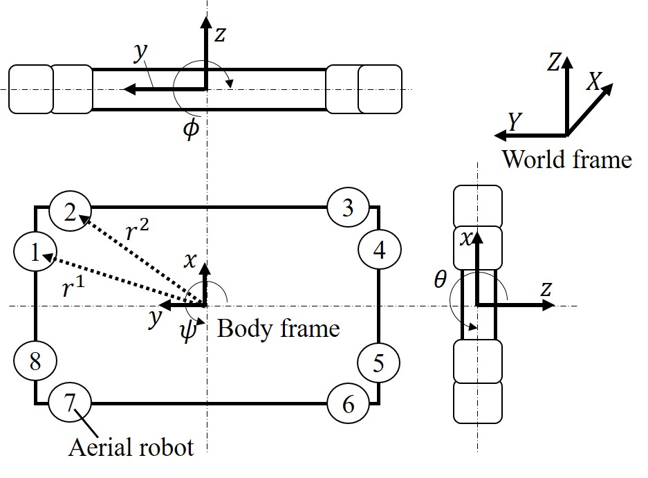
The dynamics of a payload transported by multiple aerial robots is modeled by considering robot failures. Specifically, as shown in Fig. 2, a configuration of eight single-rotor robots attached to a rectangular carrier is considered. consider a configuration in which eight robots with one rotor are attached to a rectangular carrier. The dynamics in the body frame can be approximated around a hovering condition [13] as

\displaystyle\begin{split}m\left[\begin{array}[]{c}\ddot{x}\\ \ddot{y}\\ \ddot{z}\\ \end{array}\right]=&\left[\begin{array}[]{ccc}mg&0&0\\ 0&-mg&0\\ 0&0&0\\ \end{array}\right]\left[\begin{array}[]{c}\theta\\ \phi\\ \psi\\ \end{array}\right]\\ &+\left[\begin{array}[]{c}0\\ 0\\ \sum_{i=1}^{8}\sigma_{i}u_{i}\\ \end{array}\right]+\left[\begin{array}[]{c}0\\ 0\\ -mg\\ \end{array}\right]\\ \bm{J}\left[\begin{array}[]{c}\ddot{\phi}\\ \ddot{\theta}\\ \ddot{\psi}\\ \end{array}\right]=&\left[\begin{array}[]{ccc}\sigma_{1}r^{1}_{2}&\dots&\sigma_{8}r^{8}_{2}\\ \sigma_{1}r^{1}_{1}&\dots&\sigma_{8}r^{8}_{1}\\ \sigma_{1}d_{1}c_{q}&\dots&\sigma_{8}d_{8}c_{q}\\ \end{array}\right]\left[\begin{array}[]{c}u_{1}\\ \vdots\\ u_{8}\\ \end{array}\right],\end{split}

(1)

where $x$ , $y$ , and $z$ are the three dimensional positions of the payload on the body frame system; $\phi$ , $\theta$ , and $\psi$ are the roll, pitch, and yaw angles of the payload, respectively; $u_{i}(i=1,2,\dots,8)$ is the thrust of the robot $i$ ; $m$ and $\bm{J}$ are the mass and moment of inertia of a payload, respectively; $\bm{r^{i}}(=[r^{i}_{1},r^{i}_{2}]^{\top})$ $(i=1,2,\dots,8)$ is the vector from the origin of the body frame system, COM position of the payload, to the attachment position of the robot $i$ ; $\sigma_{i}(\in\{0,1\}(i=1,2,\dots,8))$ is the failure parameter of the robot $i$ , and $\sigma_{i}=0$ when robot $i$ fails; $d_{i}(i=1,2,\dots,8)$ is the rotational direction of the robot $i$ . Furthermore, $c_{q}$ is the thrust torque conversion coefficient and $g$ is the gravitational acceleration.

We consider the dynamics of tracking error to four references, $x_{r}$ , $y_{r}$ , $z_{r}$ , and $\psi_{r}$ in the body frame. For the robust feedback controller proposed in the next section, the average thrust of the robots in each quadrant is introduced as $u_{12}=(u_{1}+u_{2})/2$ , $u_{34}=(u_{3}+u_{4})/2$ , $u_{56}=(u_{5}+u_{6})/2$ , $u_{78}=(u_{7}+u_{8})/2$ . Here, in this paper, the following is assumed:

•

The robots in each quadrant hold almost the same position, in other words, $r^{i_{1}}=r^{i_{2}}=r^{i_{1}i_{2}}(i_{1}\in\{1,3,5,7\},i_{2}=i_{1}+1)$ for the system with eight robots.
•

The rotational directions of the robots in each quadrant are same.

As a result, the error dynamics is obtained from eq. (1) as

\dot{\bm{\xi}}=\bm{A}\bm{\xi}+\bm{B_{(m,r,\sigma)}}(\bm{U}-\bm{U_{r}}),

(2)

where $\bm{\xi}=[x_{e},\dot{x}_{e},\theta_{e},\dot{\theta}_{e},y_{e},\dot{y}_{e},\phi_{e},\dot{\phi}_{e},z_{e},\dot{z}_{e},\psi_{e},\dot{\psi}_{e}]^{\top}$ , $x_{e}=x-x_{r}$ , $y_{e}=y-y_{r}$ , $z_{e}=z-z_{r}$ , $\phi_{e}=\phi-\phi_{r}$ , $\theta_{e}=\theta-\theta_{r}$ , $\psi_{e}=\psi-\psi_{r}$ . $\phi_{r}$ and $\theta_{r}$ is the references corresponding to $y_{r}$ and $x_{r}$ , respectively. $\bm{U}(=[u_{12},u_{34},u_{56},u_{78}]^{\top})$ is the input vector, $\bm{U_{r}}(=[u_{r12},u_{r34},u_{r56},u_{r78})]^{\top})$ is the stationary input vector. $\bm{A}\in\mathbb{R}^{12\times 12}$ is state matrix, $\bm{B_{(m,r,\sigma)}}\in\mathbb{R}^{12\times 4}$ is the input matrix depending on the mass of the payload, $m$ , the attachment position vector, $\bm{r}(=[r^{12},r^{34},r^{56},r^{78}]^{\top})$ , and the failure vector $\bm{\sigma}(=[\sigma_{12},\sigma_{34},\sigma_{56},\sigma_{78}]^{\top})$ . Note that $\sigma_{i_{1}i_{2}}\in\{1,2\}(i_{1}\in\{1,3,5,7\},i_{2}=i_{1}+1)$ .

III DECENTRALIZED CONTROL

In this section, we propose a decentralized controller for aerial transportation systems based on the ASSC only using the broadcasted error. It has been proven to be asymptotically stable when the target system is SPR in [18]. However, the target system of eq. (2) is not SPR. Therefore, first, a robust feedback controller is introduced to transform eq. (2) into an SPR system without sharing the exact mass and COM position. Next, we extend ASSC to multiple-output systems because the asymptotic stability of ASSC has been proven for single-output systems [18].

III-A Robust feedback controller

The target system with aerial robots is not SPR. Therefore, a state feedback control input $\bm{U_{f}}(=-\bm{F}\bm{\xi})\in\mathbb{R}^{4}$ is added to the ASSC input $\bm{U_{s}}\in\mathbb{R}^{4}$ to transform the system into an SPR one [19]. Here, $\bm{F}\in\mathbb{R}^{4\times 12}$ is the feedback gain. As a result, eq. (2) is described as

\dot{\bm{\xi}}=\bm{A}\bm{\xi}+\bm{B_{(m,r,\sigma)}}(\bm{U_{f}}+\bm{U_{s}}-\bm{U_{r}}).

(3)

Moreover, we introduce the weighted prediction error of $\bm{\xi}$ , $\bm{\zeta}\in\mathbb{R}^{4}$ for four references as follows;

\bm{\zeta}=\bm{C_{0}}\bm{\xi}+\bm{D_{0}}(\bm{U_{f}}+\bm{U_{s}}-\bm{U_{r}}),

(4)

where $\bm{C_{0}}\in\mathbb{R}^{4\times 12}$ and $\bm{D_{0}}\in\mathbb{R}^{4\times 4}$ . Note that the introduction of $\bm{D_{0}}$ corresponds to reduce the relative degree of the transportation system to zero. To obtain the feedback gain $\bm{F}$ without sharing the exact $m$ and $r$ , even if one fails, the matrix $\bm{G}\in\mathbb{R}^{4\times 4}$ is also designed. As a result, $\bm{\zeta}$ of eq. (4) is transformed into

\displaystyle\bm{\eta}=\bm{G}\bm{\zeta},

(5)

where $\bm{\eta}\in\mathbb{R}^{4}$ is the output for the ASSC. In the following, the subscript of $\bm{B}$ will be omitted for readability.

The target system consisting of eqs. (3) and (5) are SPR if there exist $\bm{F}$ , $\bm{G}$ , and positive definite symmetric matrices $\bm{P}\in\mathbb{R}^{12\times 12}$ satisfying the conditions:

\displaystyle\begin{split}&\bm{P}(\bm{A}-\bm{B}\bm{F})+(\bm{A}-\bm{B}\bm{F})^{\top}\bm{P}+\\ &\quad(\bm{P}\bm{B}-(\bm{G}\bm{C_{0}})^{\top})(\bm{G}\bm{D_{0}}+(\bm{G}\bm{D_{0}})^{\top})^{-1}\times\\ &\quad\quad(\bm{P}\bm{B}-(\bm{G}\bm{C_{0}})^{\top})^{\top}<0.\end{split}

(6)

Because eq. (6) cannot be directly solved as a linear matrix inequality (LMI) problem, eq. (6) is converted into

\displaystyle\left[\!\begin{array}[]{cc}\bm{A}\bm{Q}\!+\!\bm{Q}\bm{A}^{\top}\!\!-\!\bm{B}\bm{R}\!-\!\bm{R}^{\top}\bm{B}&\bm{Q}\bm{C_{0}}^{\top}\!\!-\!\bm{B}\bm{S}^{\top}\\ \bm{C_{0}}\bm{Q}\!-\!\bm{S}\bm{B}^{\top}&-\bm{D_{0}}\bm{S}^{\top}\!\!-\!\bm{S}\bm{D_{0}}^{\top}\\ \end{array}\!\right]<0,

(9)

where is $\bm{Q}(=\bm{P}^{-1})\in\mathbb{R}^{12\times 12}$ , $\bm{R}(=\bm{F}\bm{Q})\in\mathbb{R}^{4\times 12}$ , and $\bm{S}(=\bm{G}^{-1})\in\mathbb{R}^{4\times 4}$ are found [19].

Matrix $\bm{B}$ depends on $m$ , $\bm{r}$ , and $\bm{\sigma}$ . To transform eq. (9) into an SPR system without sharing these exact values, eq. (9) is solved so that it is satisfied with multiple $\bm{B}$ ’s simultaneously, which indicate the vertices of regions of $m$ , $\bm{r}$ , and $\bm{\sigma}$ .

III-B ASSC for multiple-output systems

For the decentralized ASSC, the direct term $\bm{G}\bm{D_{0}}(\bm{U_{f}}+\bm{U_{s}}-\bm{U_{r}})$ are approximated by

\displaystyle\bm{\zeta}\simeq\bm{C_{0}}\bm{\xi}+\hat{\bm{D}}_{0}\left[\begin{array}[]{cccc}\ddot{\hat{\theta}}&\ddot{\hat{\phi}}&\ddot{\hat{z}}&\ddot{\hat{\psi}}\\ \end{array}\right]^{\top},

(11)

where $\hat{\bm{D}}_{0}\in\mathbb{R}^{4\times 4}$ . Using $\bm{\eta}$ of eq. (5) with eq. (11), the ASSC for multiple outputs is represented by

\displaystyle\begin{split}\Sigma_{ASSC}\left\{\begin{array}[]{l}\dot{\varphi}_{i}=-K_{i}\eta_{i}\\ u_{si}=\delta(\varphi_{i})=\left\{\begin{array}[]{l}U_{p}:\varphi_{i}\geq\varphi_{pi}\\ \frac{U_{p}}{\varphi_{pi}}:0\leq\varphi_{i}<\varphi_{pi}\\ U_{n}:\varphi_{i}<0\end{array}\right.\end{array}\right.,\end{split}

(12)

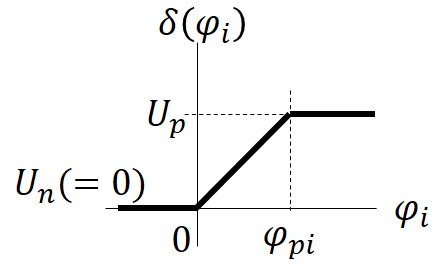
where $\eta_{j_{1}}=\eta_{j_{2}}=\eta_{j_{1}j_{2}}$ for $j_{1}=\{1,2,5,6\}$ and $j_{2}=j_{1}+1$ , $K_{i}>0$ are the gains; $u_{si}$ is the control input of ASSC of the robot $i$ ; the $U_{p}$ and $U_{n}$ are the upper and lower limits of the thrust applied by the robot, respectively; and $\delta$ is switching function of $\varphi_{i}$ as shown in Fig. 3. For the rotor without reversal, $U_{p}$ is the maximum thrust, and $U_{n}$ is $0$ . $\varphi_{pi}$ is the range of $\varphi_{i}$ from zero to $U_{p}$ . Note that the action of the robot $i$ can be adjusted by the initial values of $\varphi_{i}$ and $K_{i}$ .

For ASSC of eq. (12) for multiple-output systems, the following theorem holds.

Theorem III.1.

Eq. (3) is assumed to be transformed into a strictly positive real system by $\bm{U_{f}}.$ Using ASSC of eq. (12), the tracking error $\bm{\eta}$ satisfies $\bm{\eta}\rightarrow 0$ as $t\rightarrow\infty$ .

Proof.

For simplicity, consider the case where eq. (12) has a binary output. The storage function is defined as

\displaystyle V_{i}^{c}=\sum_{i=1}^{8}\int_{0}^{\varphi_{i}}\frac{\delta(\varphi_{i})-u_{ri}}{2K_{i}}d\varphi_{i}

(13)

where $K_{i}$ $(i=1,\dots,8)$ are constants, and $u_{ri}\in[Un,Up]$ . The derivative of eq. (13) is

\displaystyle\begin{split}\dot{V}^{c}&=\sum_{i=1}^{8}\frac{\delta(\varphi_{i})-u_{ri}}{2K_{i}}\dot{\varphi}_{i}=\sum_{i=1}^{8}\frac{u_{ri}-u_{si}}{2}\eta_{i}\\ &=-\bm{\eta}^{\top}(\bm{U_{s}}-\bm{U_{r}})\end{split}

which demonstrates the passivity. As a result, the asymptotic stability of the error is guaranteed for ASSC. See Amano et al. [18] using hyperstability theorem [20, 21] for the continuous value output in eq. (12). ∎

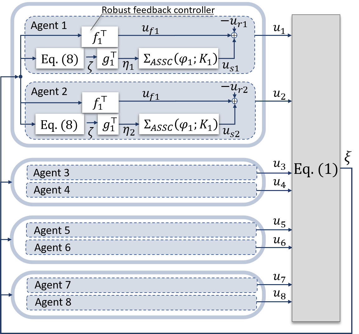
III-C Decentralized control system

Figure 4 shows the configuration of the entire control system. In this paper, by sharing the attachment positions among the robots, each robot can calculate eq. (9) by itself. Here, the expected fluctuations of $m$ , $\bm{r}$ , and $\bm{\sigma}$ are also shared among robots.

IV SIMULATION

Simulations with eight robots were performed using rectangular and L-shaped payloads. The controller was designed considering the deviations of the mass and the COM position along the $x$ and $y$ axes, and robot failures. For the control design, the equivalent position of robots in each quadrant was used. During the simulations, flights with mass and COM bias and robot failures were performed to validate the proposed method.

IV-A Condition

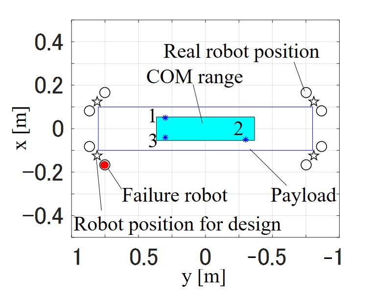
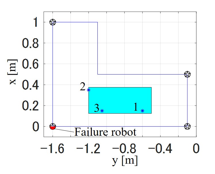
Figure 5 shows the two object shapes used for the simulations. The rectangular shape is similar to the prototype described in Section V. For the L-shape, the position of the robots used in the control design and actual design were the same. The maximum thrust of the aerial robot was set to $20$ N. The expected fluctuations were as follows: $m\in[1\quad 3]$ kg; the number of failed robots was one; the COM range was shown in Fig. 5. The parameters of ASSC were as follows: $U_{p}=20$ N; $U_{n}=0$ N; $K_{i}=10\quad(i=1,\dots,8)$ for the rectangle shape; $K_{i}=20\quad(i=1,\dots,8)$ for the L-shape. In the simulation, the flights to the references were performed with three paired masses and COM positions $(m,\rm{COM})\in\{(2,\rm{COM1}),(1,\rm{COM2}),(3,\rm{COM3})\}$ , as shown in Fig. 5. Furthermore, one robot was stopped after $2.5$ s to simulate the failure. The references, $X_{r}$ , $Y_{r}$ , and $Z_{r}$ in the world frame, and $\psi_{r}$ in the body frame were $3.0$ m, $2.0$ m, $1.0$ m, and $0.3$ rad, respectively. $X_{r}$ , $Y_{r}$ , and $Z_{r}$ are transformed into $x_{r}$ , $y_{r}$ , and $z_{r}$ in the body frame. The initial position of $z$ was set to $1.0$ m, and the others were set to zero.

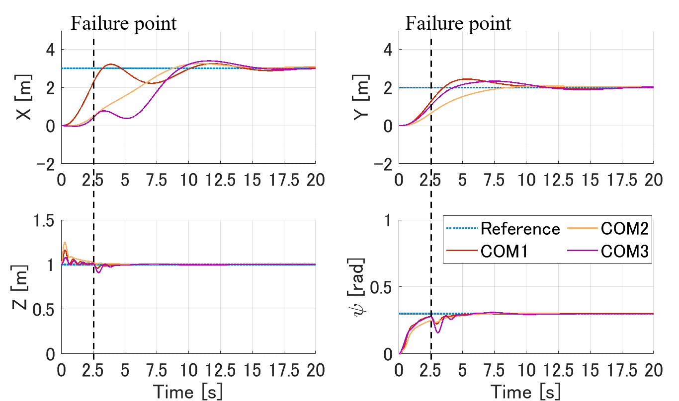
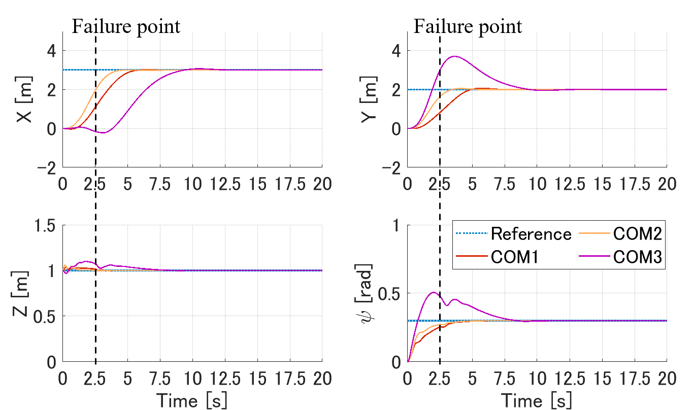
IV-B Result

Figure 6 shows the results of three simulations. The positions and yaw angle of the payload reached the references, even if the mass and the COM are biased and robot failure occurred. For both shapes, there was a large fluctuation in the case of COM3. This is because the COM position is closest to the failed robot. Since the L-shape is unbalanced, it tends to fluctuate more than the rectangle shape. The fluctuation of the rectangle shape is larger only in the $X$ -direction, because there is no margin in the moment arm in the $x$ -direction.

V EXPERIMENT

To verify our method with actual robots, a prototype was manufactured for use in practical experiments. The experiment was performed under two conditions. First, we verify the aerial transportation using both the robust feedback controller and ASCC. Next, the aerial transformation without the robust feedback controller is verified.

V-A Prototype

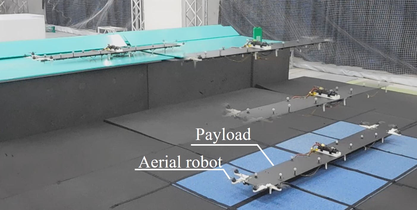
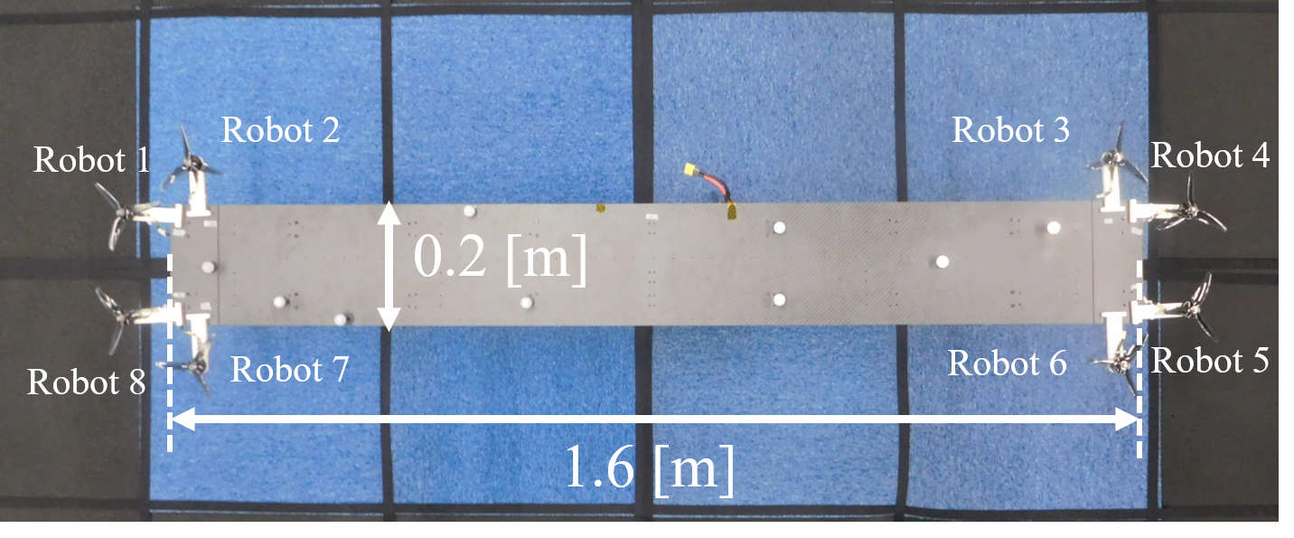
The prototype consisted of a rectangular payload and eight aerial robots, as shown in Fig. 8. Each aerial robot consisted of one rotor and an arm connected to the transported payload. Each robot was controlled by a single flight controller (PIXHAWK [22]) mounted on the transported payload. When distributed control was implemented, the control input of each robot was calculated independently by the flight controller. The software that included our method was coded by MATLAB Simulink and Stateflow, and implemented in the flight controller. In addition, the position of the payload was obtained from the motion capture system, and the attitude was obtained from the inertial measurement unit (IMU) in the flight controller. The COM position and the mass of the payload was changed by using the battery and an additional weight. The size of the payload was $1.6\times 0.2$ m, and the mass excluding the robot and battery was approximately $1.9$ kg. The maximum thrust of one aerial robot is $14.2$ N according to the motor manufacturer’s specification value.

V-B Condition

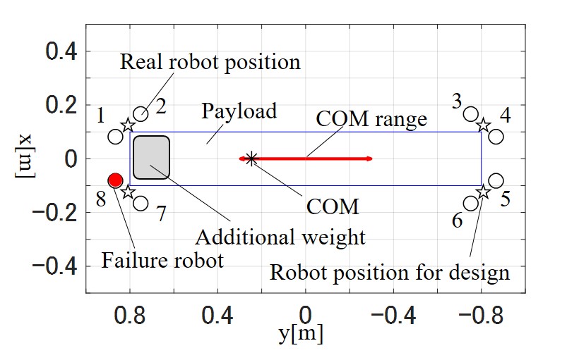
The controller was designed considering deviations in the COM along the $y$ -axis, and a robot failure, as shown in Fig. 8. When the prototype was loaded with an additional weight, the COM was biased by $0.25$ m in the $y$ -direction, and the total mass of the prototype with an additional weight was $2.7$ kg. First of the transportation experiments, the goal of the reference position was a platform $0.5$ m high ( $Z_{r}=0.5$ ) and $3$ m ahead ( $X_{r}=3$ ).

Next, in the failure experiment, we stopped one robot during transportation, as shown in Fig. 8. Finally, in the fully distributed controller without sharing the attachment positions of robots, the feedback control input $\bm{U_{f}}$ , shown in Fig. 4, was set to zero. Here, the experiment was conducted while hovering and the COM was centered. In all experiments, measurement data was recorded in a $200$ ms cycle.

V-C Result

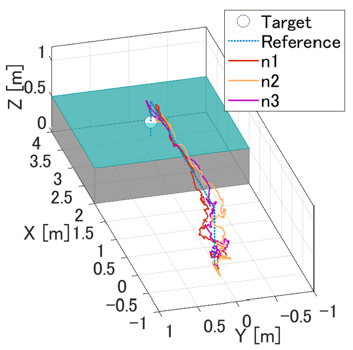
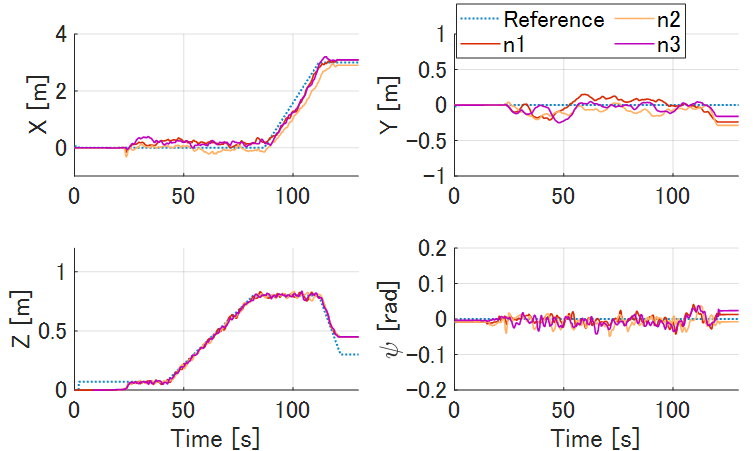
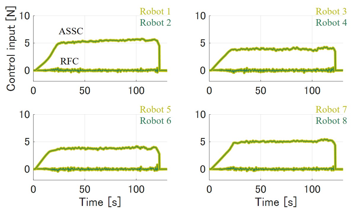
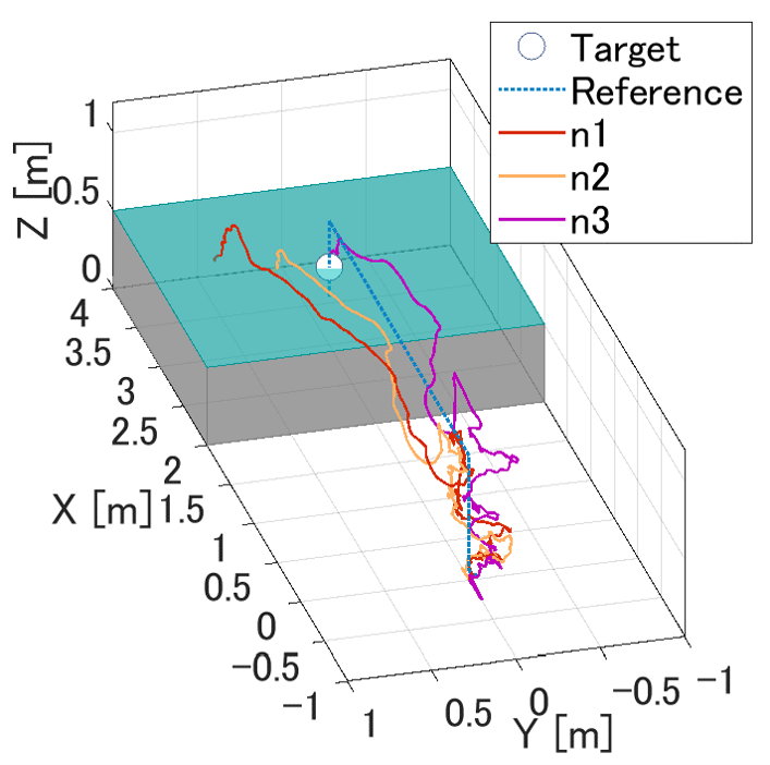
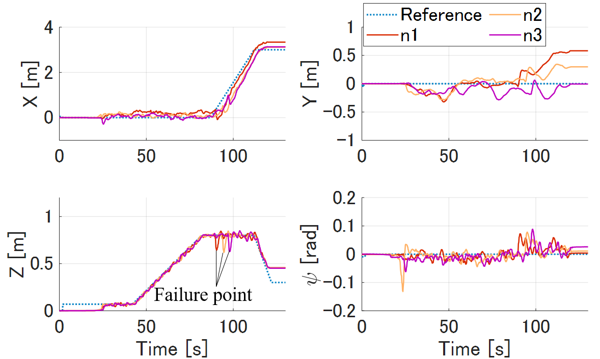
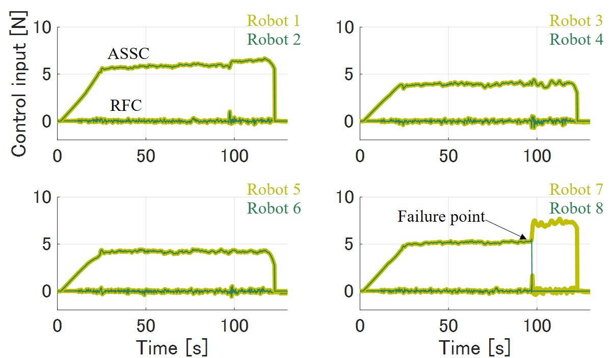
Figure 9 shows the results of the aerial transportation with a biased COM and a robot failure. The results confirmed that the proposed method enables the tracking control to the reference, even if the COM is biased and a robot fails. In the robot failure experiment, the altitude dropped immediately after the failure, but the prototype quickly returned to the reference position. The robust feedback inputs of eight robots are almost zero except for the unsteady state at the time of failure, and is as small as $2$ N or less even at the time of failure. In other words, most of the flight control is processed by ASSC. In addition, ASSC instantly compensates for the shortage of thrust in the event of a failure. On the other hand, offsets in the $Y$ -direction were observed at the time of failure. This offset occurred when the prototype enters a dead band of control owing to fluctuations caused by the failure.

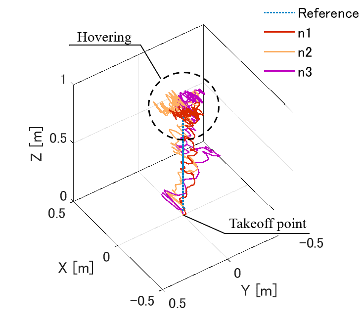
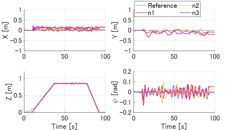
Figure 10 shows the results without the robust feedback input $\bm{U_{f}}$ . In this case, the prototype took off, hovered, and landed even with fully decentralize control, although the asymptotic stability was not proven.

VI CONCLUSIONS

In this study, we proposed a novel decentralized controller based ASSC for unstable transportation systems. First, a feedback controller was introduced to transform the unstable system into an SPR system by sharing the attachment positions among the robots. This controller is robust against expected fluctuations (mass, COM, and failures). Next, the asymptotic stability of ASSC of multiple outputs to the references was proven. The effectiveness was confirmed by simulations with rectangular and L-shape payloads. Furthermore, cooperative transportation is demonstrated using a prototype with a payload larger than the robots, even under robot failure. Finally, it was shown that the proposed system carried an unknown payload, even if the attachment positions were not shared.

The limitation of the proposed method is that the robots in each quadrant hold almost the same position. In the future, we would like to relax this assumption. Moreover, in this paper, the distributed processing was performed on the software. Therefore, we would like to decentralize it on hardware by manufacturing the system in which each robot has a microcomputer.

References

[1] V.Kumar and N.Michael, “Opportunities and challenges with autonomous micro aerial vehicles,” The International Journal of Robotics Research, vol. 31, no. 11, pp. 1279–1291, Aug. 2012.
[2] A. Ollero, J. Cortes, A. Santamaria-Navarro, M. A. T. Soto, R. Balachandran, J. Andrade-Cetto, A. Rodriguez, G. Heredia, A. Franchi, G. Antonelli, K. Kondak, A. Sanfeliu, A. Viguria, J. R. Martinez-de Dios, and F. Pierri, “The AEROARMS project: Aerial robots with advanced manipulation capabilities for inspection and maintenance,” IEEE Robotics & Automation Magazine, vol. 25, no. 4, pp. 12–23, Dec. 2018.
[3] F. Ruggiero, V. Lippiello and A. Ollero, “Aerial manipulation: A literature review,” IEEE Robotics and Automation Letters, vol. 3, no. 3, pp. 1957–1964, Jul. 2018. IEEE Robotics & Automation Magazine, vol. 25, no. 4, pp. 12-23, Dec. 2018.
[4] E. Ackerman and M. Koziol, “The blood is here: Zipline’s medical delivery drones are changing the game in rwanda,” IEEE Spectrum, vol. 56, no. 5, pp. 24–31, 2019.
[5] D. K. Villa, A. S. Brandão and M. Sarcinelli-Filho, “A survey on load transportation using multirotor uavs,” Journal of Intelligent & Robotic Systems, vol. 80, pp. 267–296, 2020.
[6] S. Chung, A. A. Paranjape, P. Dames, S. Shen and V. Kumar, “A survey on aerial swarm robotics,” IEEE Transactions on Robotics, vol. 34, no. 4, pp. 837–855, Aug. 2018.
[7] N.Michael, J. Fink, and V. Kumar, “Cooperative manipulation and transportation with aerial robots,” Autonomous Robots, vol. 30, no. 1, pp. 73–86, Sep. 2010.
[8] Q. Jiang and V. Kumar, “The inverse kinematics of cooperative transport with multiple aerial robots,” in IEEE Transactions on Robotics vol. 29, no. 1, pp. 136–145, 2013.
[9] K. Klausen, C. Meissen, T. I. Fossen, M. Arcak, and T. A. Johansen, “Cooperative control for multirotors transporting an unknown suspended load under environmental disturbances,” IEEE Transactions on Control Systems Technology, 2018.
[10] M. Gassner, T. Cieslewski, and D. Scaramuzza, “Dynamic collaboration without communication: Vision-based cable-suspended load transport with two quadrotors,” in 2017 IEEE International Conference on Robotics and Automation (ICRA), pp. 5196–-5202, IEEE, 2017.
[11] A. Tagliabue, M. Kamel, S. Verling, R. Siegwart, and J. Nieto, “Collaborative transportation using MAVs via passive force control,” in 2017 IEEE International Conference on Robotics and Automation (ICRA), pp. 5766–-5773, IEEE, 2017.
[12] J. Wehbeh, S. Rahman and I. Sharf, “Distributed model predictive control for UAVs collaborative payload transport,” in 2020 IEEE/RSJ International Conference on Intelligent Robots and Systems (IROS), pp. 11666–11672, IEEE, 2020.
[13] D. Mellinger, M. Shomin, N. Michael, and V. Kumar, “Cooperative grasping and transport using multiple quadrotors,” Distributed autonomous robotic systems., pp. 545–558, Springer, 2013.
[14] G. Loianno and V. Kumar, “Cooperative transportation using small quadrotors using monocular vision and inertial sensing,” IEEE Robotics and Automation Letters, vol. 3, no. 2, pp.680–687, 2018.
[15] B. Gabrich, D. Saldana, V. Kumar, and M. Yim, “A flying gripper based on cuboid modular robots,” in 2018 IEEE International Conference on Robotics and Automation (ICRA), pp. 7024–-7030 IEEE, 2018.
[16] Z. Wang, S. Singh, M. Pavone, and M. Schwager, “Cooperative object transport in 3d with multiple quadrotors using no peer communication,” in 2018 IEEE International Conference on Robotics and Automation (ICRA), pp. 1064–-1071. IEEE, 2018.
[17] K. Oishi and T. Jimbo “Autonomous Cooperative Transportation System involving Multi-Aerial Robots with Variable Attachment Mechanism,” in 2021 IEEE/RSJ International Conference on Intelligent Robots and Systems (IROS), (in press), IEEE, 2021.
[18] Y. Amano, T. Jimbo, and K. Fujimoto, “Tracking Control for Multi-Agent Systems Using Broadcast Signals based on Positive Realness,” arXiv preprint arXiv:2109.06372, 2021.
[19] A. van der Schaft, “L2-gain and passivity techniques in nonlinear control,” (Vol. 2). London: Springer, 2017.
[20] B. Anderson, “A simplified viewpoint of hyperstability,” IEEE Transactions on Automatic Control, vol. 13, no. 3, pp. 292–-294, 1968.
[21] I. D. Landau, “Adaptive control: the model reference approach,” Marcel Dekker, New York, 1979.
[22] M. Lorenz, P. Tanskanen, L. Heng, G. H. Lee, F. Fraundorfer, and M. Pollefeys, ”PIXHAWK: A system for autonomous flight using onboard computer vision,” in 2011 IEEE International Conference on Robotics and Automation (ICRA), pp. 2992–2997, IEEE, 2011.