Cooperative Extended State Observer Based Control of Vehicle Platoons With Arbitrarily Small Time Headway
Abstract
We study platoon control of vehicles with linear third-order longitudinal dynamics under the constant time headway policy. The controller of each follower vehicle is only based on its own velocity, acceleration, inter-vehicle distance and velocity difference with respect to its immediate predecessor, which are all obtained by on-board sensors. We develop distributed cooperative extended state observers for followers to estimate the acceleration differences between adjacent vehicles. Based on estimates of the acceleration differences, distributed cooperative control laws are designed. By using the stability theory of perturbed linear systems, we show that the control parameters can be properly designed to ensure the closed-loop and string stabilities for any given positive time headway. We further show that the proposed control law based on the ideal vehicle model can guarantee the closed-loop and string stabilities even if there are small model parameter uncertainties. Also, simulation results demonstrate the robustness of the proposed control law against sensing noises, input delays and parameter uncertainties.
keywords:
Vehicle platoon; Constant time headway; Extended state observer; String stability., ,*, ,
1 Introduction
Vehicle platoon can improve road utilization rate and reduce fuel consumption effectively (Alam, 2011). Therefore, it has attracted worldwide attention (Shladover et al., 1991; Coelingh & Solyom, 2012). From networked control perspective, Li et al. (2015) divided a vehicle platoon system into four basic modules: node dynamics, information flow topology, formation geometry, and distributed controller, among which the formation geometry greatly affects the stability of the vehicle platoon system. Formation geometry is determined by the spacing policy. The constant time headway policy is considered by Klinge & Middleton (2009); Naus et al. (2010); Xiao & Gao (2011); Ploeg et al. (2014); Darbha et al. (2017) and it is well known that a large time headway is conducive to string stabilities of vehicle platoon system (Rajamani & Zhu, 2002; Naus et al., 2010), however, the larger the time headway is, the greater the inter-vehicle distance becomes, which leads to a lower road utilization rate.
It is of interest to guarantee the stability of the vehicle platoon with small time headways. Many researches showed that using the accelerations of the preceding vehicles can reduce the lower bound of the time headway required (Rajamani & Zhu, 2002; Zhou & Peng, 2004; Naus et al., 2010; Darbha et al., 2017; Al-Jhayyish & Schmidt, 2018). All the above works assumed that the accelerations of the preceding vehicles are obtained by the wireless communication network accurately, however, accurate communication doesn’t exist in practical applications. In addition, a control law which relies on communication data runs the risk of failure when the inter-vehicle communication network breaks down under attack. Therefore, a cooperative control law with a small time headway, which can ensure both closed-loop and string stabilities without relying on the inter-vehicle wireless communication network, is of especially significance for practical applications. Ploeg et al. (2015) and Wen & Guo (2019) proposed methods to estimate the acceleration differences between adjacent vehicles, respectively. The control laws in Ploeg et al. (2015) and Wen & Guo (2019) are indeed independent of wireless communication networks. The closed-loop and string stabilities are analyzed by numerical simulations in Ploeg et al. (2015) and Wen & Guo (2019), especially, Ploeg et al. (2015) considered a third-order linear model with input delays, in which the simulation results show that the string stability is not guaranteed if the time headway is small enough.
In this paper, we study platoon control of vehicles with linear third-order longitudinal dynamics under the constant time headway policy. We design a distributed cooperative control law for each follower vehicle only using its own velocity, acceleration, inter-vehicle distance and velocity difference with respect to its immediate predecessor, all of which can be obtained by on-board sensors. Firstly, the models of velocity difference between adjacent vehicles are established, based on which distributed cooperative extended state observers are designed to estimate the acceleration differences between adjacent vehicles. Then based on these estimates, distributed cooperative controllers are designed for follower vehicles. The controller for each follower consists of two parts, where the first part is a feedback term consisting of inter-vehicle distance error and its differential, the other is a feedforward term consisting of the estimate of the acceleration of the preceding vehicle. Thus, the whole cooperative control law only uses the data obtained by on-board sensors without wireless communication networks.
We analyze both closed-loop and string stabilities of the vehicle platoon system. The closed-loop system matrix is decomposed into two matrices, one of which is related to feedback parameters of the distributed controllers, and the other is regarded as the perturbation matrix, which is related to feedforward parameters. Then, we give the range of the control parameters to ensure the closed-loop stability by using the stability theory of perturbed linear systems. In the frequency domain, we analyze the transfer functions which describe the inter-vehicle distance error propagation, and give the range of the control parameters to ensure the string stability. We show that one can design control parameters properly to ensure both closed-loop and string stabilities for any given positive time headway. Our method for estimating the acceleration differences between adjacent vehicles is based on distributed cooperative extended state observers, which is totally different from those in Ploeg et al. (2015) and Wen & Guo (2019). Besides, we give the explicit range of control parameters quantitatively related to the system parameters to ensure both closed-loop and string stabilities for any given positive time headway.
We analyze the robustness of the proposed control law by both theoretical study and numerical simulations. (i) The proposed control law guarantees the exponential closed-loop stability, thus it is naturally robust against bounded sensing noises. (ii) We show that the proposed cooperative control law based on the ideal vehicle model can still ensure the closed-loop and string stabilities provided the parameter uncertainties in the vehicle model are sufficiently small. (iii) In the numerical simulations, we consider the same vehicle model with input delays and the same time headway as Ploeg et al. (2015), with additional sensing noises and uncertain model parameters. Simulation results show that the closed-loop and string stabilities can be guaranteed by the proposed control law based on the ideal vehicle model.
The rest of this paper is organized as follows. The vehicle model and the control objectives are presented in Section II. In Section III, we first establish dynamic models based on velocity differences between every adjacent vehicles, then distributed cooperative extended state observers are designed to estimate the acceleration differences between adjacent vehicles. Finally, distributed cooperative controllers for follower vehicles are designed. In Section IV, we give the range of control parameters for the closed-loop and string stabilities. In Section V, we analyze the robustness of the proposed control law against model parameter uncertainties. Numerical simulations are carried out in Section VI. In Section VII, we give some conclusions.
The following notation will be used throughout this paper. For a given matrix , its 2-norm and minimum singular value are denoted by and , respectively; denotes a block diagonal matrix whose diagonal blocks are all matrix ; denotes the complex domain; denotes the real domain; and denote a zero matrix and an identity matrix with an appropriate size, respectively. For a given transfer function , its -norm and inverse Laplace transform are denoted by and , respectively.
2 Problem formulation
We consider the following third-order linear vehicle model which is commonly used in the vehicle platoon control (Rajamani & Zhu, 2002; Ploeg et al., 2015; Zheng et al., 2016; Wen & Guo, 2019).
| (1) |
where , and are the position, velocity and acceleration of the th vehicle, respectively, is the control input of the leader vehicle and is the control input of the th follower vehicle to be designed, . The constant is the inertial delay of vehicle longitudinal dynamics. We consider the constant time headway spacing policy. The expected inter-vehicle distance is denoted by
| (2) |
where the constants and are the standstill distance and the time headway, respectively. The inter-vehicle distance error is given by,
| (3) |
which is the difference between the actual inter-vehicle distance and the expected inter-vehicle distance. Denote , where is the Laplace transform of . The control objectives are to design , , for follower vehicles so that the following two objectives are satisfied.
A. closed-loop stability: all the follower vehicles tend to move at the same velocity as the leader vehicle and the inter-vehicle distance errors converge to zero, i.e. , .
B. string stability: the inter-vehicle distance errors are not amplified during the backward propagation along the platoon, i.e.
3 Cooperative control law based on extended state observer
Suppose that there is no wireless communication between vehicles. We consider predecessor following topology, and each follower vehicle in the platoon relies on the on-board sensors to measure its own velocity, acceleration, the inter-vehicle distance and the velocity difference with respect to its immediate predecessor. However, the sensor of each follower vehicle cannot measure the acceleration of its immediate predecessor. Instead, we can design an observer to estimate the acceleration difference between adjacent vehicles. The extended state observer (ESO) was first put forward by Han (1995), whose core idea is to expand the unmodeled dynamics into new state and then according to the new state equation, an extended state observer is designed to estimate all states of the system. However, the extended state observer proposed by Han (1995) is nonlinear, which has difficulty in parameter tuning and stability analysis. Gao (2003) put forward a linear extended state observer, which simplifies parameter tuning and is also beneficial for stability analysis. In this paper, we design a linear extended state observer to estimate the acceleration difference between adjacent vehicles.
According to (1), the models of the velocity difference between adjacent vehicles are given by
| (4) |
where
| (5) | ||||
| (6) | ||||
| (7) | ||||
| (8) |
Here, is the unmodeled dynamics, which contains the control input and the acceleration of th vehicle that cannot be measured directly by the th vehicle. We design a linear extended state observer
| (9) |
where is the estimate of the acceleration difference between the th vehicle and the th vehicle. The constants , and are the observer gains to be designed. Then by the acceleration of th vehicle, the estimate of the acceleration of th vehicle is given by . The controller of th follower vehicle is designed as
| (10) |
where , , are the control parameters to be designed. The controller (3) consists of two parts. The first part is the feedback item, which consists of the inter-vehicle distance error between the adjacent vehicles and its differential; while the second part is the feedforward item, which consists of the estimate of the acceleration of the th vehicle. It can be seen that the extended state observer (9) and the controller (3) only use the information obtained by on-board sensors of followers.
4 Stability analysis of vehicle platoon
In reality, the velocity of the leader vehicle will reach at a steady state within a finite time , that is, there exists , such that , . We make the following assumption.
Assumption 1.
.
Denote , where , and are dimensional matrices with ,
For the closed-loop and string stabilities, we have the following theorems.
Theorem 1.
Remark 4.1.
Theorem 1 shows that the control law (9) and (3) can be properly designed such that the closed-loop system is exponentially stable, so the proposed control law is naturally robust against sensing noises, i.e. under the control law (9) and (3) with bounded sensing noises in the measurements of , and , the inter-vehicle distance errors will converge to a neighborhood of zero whose size is proportional to the noise intensities.
Theorem 2.
Remark 4.2.
Remark 4.3.
Theorem 2 shows that the control parameters can be properly designed to ensure the string stability for any given positive time headway. There is another definition of string stability, called string stability, which means . According to Eyre et al. (1998), if and , then string stability is satisfied.
Remark 4.4.
In reality, the velocity of leader vehicle is positive. According to Eyre et al. (1998), if and , where , is Laplace transform of , then , and the have the same sign as . Thus the velocities of follower vehicles are positive. The evolution of and are investigated by numerical simulation in Section 6.
5 Robustness against parameter uncertainties
The control law (9) and (3) is designed based on the ideal vehicle model (1) with completely known parameters. In practice, the vehicle model may be inaccurate. In this section, we will give the range of control parameters to ensure the closed-loop and string stabilities when there are parameter uncertainties in the vehicle model. It is shown that the control law (9) and (3) based on the ideal vehicle model can ensure the closed-loop and string stabilities with small model parameter uncertainties.
Suppose that the real vehicles have the following dynamics
| (16) |
where the definitions of are the same as in (1). The constant is the known nominal inertial delay of vehicle longitudinal dynamics. The constant is the parameter uncertainty. We assume that , , where . We have the following theorems.
Theorem 3.
Theorem 4.
Remark 5.5.
From Theorem 3, we know that the control law (9) and (3) is robust against model parameter uncertainties. If , then (23) holds and (27) degenerates into (12). By the continuity of (23) and (27) with respect to , we know that if the control law (9) and (3) is designed according to Theorem 1 based on the ideal vehicle model (1), then the closed-loop and string stabilities can be ensured provided is sufficiently small.
Remark 5.6.
A more accurate nonlinear vehicle model is considered in Zheng et al. (2016)
| (31) |
where is the expected driving or braking torque of the th vehicle at time . The constant , , , , and are the mass, the rolling resistance coefficient, the tire radius, the total air resistance coefficient, the inertial delay of longitudinal dynamics and the mechanical efficiency of the drive train of the th vehicle, respectively. The constant is the gravitational acceleration. The feedback linearization law is given by
| (32) |
where the constants , , , , and are the nominal parameters of th vehicle, and are the velocity and acceleration of th vehicle measured by on-board sensors, and are sensing noises . Substituting (5.6) into (31), we obtain
| (33) |
where . Compared with (1), the model (33) contains a nonlinear term . From (33), we know the models of the velocity difference between adjacent vehicles (4) with . The ESO (9) can still be used to estimate the acceleration differences between adjacent vehicles. The nonlinear term can be estimated by designing another ESO
| (34) |
where , and are the estimates of , and , respectively. The constants , and are the observer gains to be designed. The controller of th follower vehicle is designed as
| (35) |
where and are the inter-vehicle distance error and velocity difference between adjacent vehicles measured by on-board sensors, and are sensing noises. The stability analysis of the vehicle platoon system (33) under control law (9), (34) and (5.6) would be an interesting and challenging topic for future investigation.
6 NUMERICAL SIMULATIONS
Suppose there are 1 leader vehicle and 5 follower vehicles with the following dynamics with parameter uncertainties
where . The parameter uncertainties are given by , , , , , .
To make the behavior of the leader vehicle close to a real vehicle, we construct a virtual vehicle in CarSim and record its acceleration. Then we use the recorded acceleration as the expected acceleration of the leader vehicle in the following simulations. The initial velocities are given by , . The initial accelerations are given by , . The initial positions are taken as , , , , , . The standstill distance is given by . Let . We choose , , and , , and . The evolution of and are shown in Fig.1.
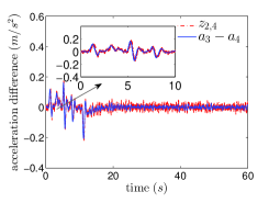
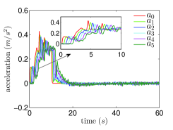
The actual and the estimated acceleration differences between the 3rd and 4th follower vehicles are shown in Fig.2(a). The evolution of vehicles’ accelerations and velocities are shown in Fig.2(b) and Fig.2(c), respectively. The evolution of inter-vehicle distance errors are shown in Fig.2(d).
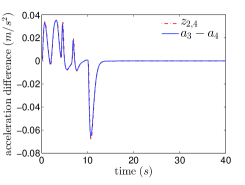
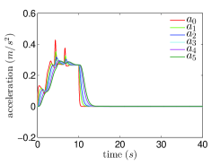
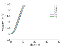
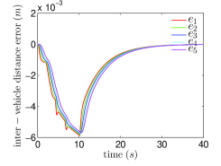
Fig.1 shows that and . Then from Remark 4.4, we know that and the have the same sign as , which are also shown in Fig.2.(c). From Fig. 2.(a), it is shown that although the ESO (9) are designed based on the nominal , the acceleration differences between adjacent vehicles can be estimated well by the ESO (9). Fig.2.(b) and Fig.2.(c) show that the accelerations of follower vehicles and velocity differences between adjacent vehicles converge to zero as the acceleration of leader vehicle goes to zero, respectively. From Fig.2.(d), it is observed that the inter-vehicle distance errors converge to zero and they are not amplified in the backward propagation along the platoon.
Next, we consider the vehicle model with input delays, i.e. the is replaced by , where is the input delay. In practical applications, the velocity differences between adjacent vehicles , , measured by on-board sensors are usually corrupted by random noises. In the numerical simulations, we implement the sampled-data version of the control law (9) and (3) with replaced by , where is the sampling period and is a sequence of random variables with the uniform distribution . We choose , , and , , and . The actual and the estimated acceleration differences between the 3rd and 4th follower vehicles are shown in Fig.3.(a). The evolution of vehicles’ accelerations, velocities and inter-vehicle distance errors are shown in Fig.3.(b), Fig.3.(c) and Fig.3.(d), respectively.
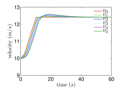
From Fig.3.(a), it is shown that although the velocity differences are corrupted by sensing noises, the sensing noises are not significantly amplified and the output of the ESO can still track the acceleration differences between adjacent vehicles . Fig.3.(b), Fig.3.(c) and Fig.3.(d) show that the accelerations of follower vehicles, velocity differences between adjacent vehicles and inter-vehicle distance errors converge to a small neighborhood of zero. Fig.3 shows the robustness of the proposed control law against parameter uncertainties, sensing noises and input delays.
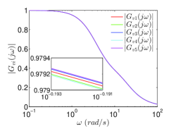
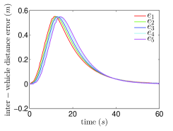
Then let the time headway change to . By Fig.4.(a), it is observed that the control law (9) and (3) with the previous parameters, i.e. , , , , and , cannot ensure the string stability any longer, but the closed-loop stability is still guaranteed.
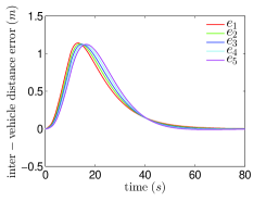
We reselect , , , , and . It can be seen from Fig.4.(b) that the closed-loop and string stabilities are both ensured by reselecting the control parameters. It is shown that for a smaller time headway , a smaller can be chosen to ensure string stability at the cost of slower convergence.
The transient performance of the closed-loop system can be investigated from the structure of the compound controller (3) containing proportional differential feedback and feedforward terms. The convergence rate of the closed-loop system is mainly determined by the proportional differential term. The feedforward term reduces the influence of disturbances.
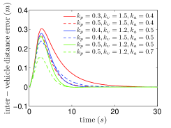
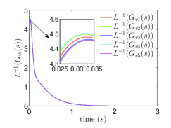
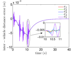
Let any two of the control parameters , and be fixed and the other one be changed. The evolution of inter-vehicle distance errors between the leader and the first follower under different control parameters are shown in Fig.5. Fig.5 shows that a larger leads to a faster convergence and a larger leads to a slower convergence with smaller inter-vehicle distance error. The parameter has little effect on the convergence rate, and a larger brings a smaller inter-vehicle distance error.
7 Conclusion
We have considered the platoon control for homogeneous vehicles with third-order linear dynamics model. The constant time headway spacing policy is adopted. Firstly, the distributed cooperative extended state observers are designed to estimate the acceleration differences between adjacent vehicles. Then the controller of each follower vehicle is designed by its own velocity, acceleration, velocity difference and estimated acceleration difference with respect to its immediate predecessor. The information required by the control law can be obtained by on-board sensors. The closed-loop stability of the vehicle platoon system is analyzed by the stability theory of perturbed linear systems, and the sufficient conditions to ensure the closed-loop stability are given. Also the string stability is analyzed in the frequency domain and the range of the control parameters that guarantee the string stability is presented. It is shown that for any given positive time headway, control parameters can be properly designed to guarantee both closed-loop and string stabilities of the vehicle platoon system. In addition, it has been shown that the closed-loop and string stabilities of the vehicle platoon system can be guaranteed with small model parameter uncertainties.
Acknowledgements
This work was supported by the National Natural Science Foundation of China under Grant 61977024 and the Basic Research Project of Shanghai Science and Technology Commission under Grant 20JC1414000.
Appendix A
Appendix B Proof of Theorem 1
The proof of Theorem 1 needs the following lemmas.
Lemma B.7.
Lemma B.8.
For any , , where is the element of the th row and th column of .
Proof. Denote
| (36) |
Define , where is the element of the th row and th column of .
By (36) and the definition of , we have
This together with the triangle inequality of matrix norm leads to
| (37) |
By the definition of the 2-norm of matrix, we have
| (38) |
where is the maximum eigenvalue of .
Proof of Theorem 1. Denote
| (39) | ||||
| (40) | ||||
| (41) | ||||
| (42) | ||||
| (43) |
where
| (44) | ||||
| (45) | ||||
| (46) | ||||
| (47) | ||||
| (48) | ||||
| (49) | ||||
| (50) |
From (6), (3) and (45), we know
| (51) |
This together with (1), (3), (5), (39) and (40) leads to
| (55) |
where
From (3), (39) and (41), we get
| (56) |
where
From (47), (55) and (56), we obtain
| (59) |
where
By (3)-(9), (40), (41), (44)-(B) and (59), we have
| (66) |
where
From (42), (43), (59) and (66), we know
| (67) |
where and
Firstly, we analyze the stability of . The eigenvalues of are only related to and . Calculating the characteristic polynomial of , we obtain
| (68) |
The Rouse table corresponding to (68) is given by
| 1 | ||
| 0 | ||
By and (11), we know that the elements of the first column of the Rouse table corresponding to (68) are all greater than zero. From Rouse criterion, is stable. Calculating the characteristic polynomial of , we get
| (69) |
The Rouse table corresponding to (69) is given by
| 1 | ||
| 0 | ||
By , , , we know that the elements of the first column of the Rouse table corresponding to (69) are all greater than zero. From Rouse criterion, is stable. Then is stable. From the definition of and Lemma 2, we know
| (73) |
From (12) and (73), we get . It is known from the definition of and Assumption 1 that . By Lemma 1 and (67), we know converges to zero exponentially. Then and both converge to zero exponentially, , which implies converges to zero exponentially, . ∎
Appendix C Proof of Theorem 2
Proof of Theorem 2. By (3) and (5), we get
| (74) |
Taking the Laplace transform of (74), we have
| (75) |
where and are the Laplace transform of , , respectively. From (1), we know
| (76) |
This together with (74) leads to
| (77) |
Taking the Laplace transform of (77), we get
| (78) |
where is the Laplace transform of . Taking the Laplace transform of (9), we have
| (83) |
where , and are the Laplace transform of , and , respectively. Substituting (78) into (83), we obtain
| (84) |
| (85) |
Taking the Laplace transform of (C), we have
| (86) |
Denote . By (75), (E) and (C), we get
| (87) |
where
| (88) |
Taking the Laplace transform of (88), we have
This together with leads to
This together with (87) leads to
| (89) |
where
Substituting into (C), we get
| (90) |
where , , , .
By and , we know and . From (15), we obtain . This together with and leads to
| (91) |
From (13) and , we know . This together with leads to . From (15), we know . This together with and leads to
| (92) |
By (13), we know . This together with leads to . By (13), we get . This leads to . By (14), we know . This together with leads to . From (15), we know . This together with and leads to
| (93) |
From (15), we obtain . This together with and leads to
| (94) |
From (15), we obtain . This together with and leads to
| (95) |
| (96) |
Through calculation, we get
This together with (C) leads to
| (97) |
Through calculation, we know
This together with (C) leads to
| (98) |
By (98), we know
| (99) |
Through calculation, we obtain
This together with (99) leads to
| (100) |
Appendix D Proof of Theorem 3
Proof of Theorem 3. For simplicity of presentation, we denote . According to (16), the models of the velocity difference between adjacent vehicles are given by
| (101) |
where the definitions of and are the same as in (4),
| (102) | ||||
| (103) |
Denote
| (104) | ||||
| (105) | ||||
| (106) | ||||
| (107) | ||||
| (108) |
where
| (109) | ||||
| (110) | ||||
| (111) | ||||
| (112) | ||||
| (113) | ||||
| (114) | ||||
| (115) |
From (6), (3) and (110), we know
| (116) |
This together with (16), (3), (5), (104) and (105) leads to
| (120) |
where
From (3), (104) and (106), we get
| (121) |
where
From (112), (120) and (121), we obtain
| (124) |
where
By (3), (5), (6), (9), (16), (102)-(106), (109)-(D) and (124), we have
| (134) |
where
From (107), (108), (124) and (134), we know
| (135) |
where and
Firstly, we analyze the stability of . The eigenvalues of are only related to and . Calculating the characteristic polynomial of , we obtain
| (136) |
The Rouse table corresponding to (136) is given by
| 1 | ||
| 0 | ||
By and (19), we know that the elements of the first column of the Rouse table corresponding to (136) are all greater than zero. From Rouse criterion, is stable. Calculating the characteristic polynomial of , we get
| (137) |
The Rouse table corresponding to (137) is given by
| 1 | ||
| 0 | ||
By , , , we know that the elements of the first column of the Rouse table corresponding to (137) are all greater than zero. From Rouse criterion, is stable. Then is stable.
Appendix E Proof of Theorem 4
Proof of Theorem 4. For simplicity of presentation, we denote . By (3) and (5), we get
| (142) |
Taking the Laplace transform of (142), we have
| (143) |
where and are the Laplace transform of , , respectively. From (16), we know
| (144) |
This together with (142) leads to
| (145) |
Taking the Laplace transform of (145), we get
| (146) |
where is the Laplace transform of . Taking the Laplace transform of (9), we have
| (151) |
where , and are the Laplace transform of , and , respectively. Substituting (146) into (151), we obtain
| (152) |
By (3), (142) and (144), we get
| (153) |
Taking the Laplace transform of (E), we have
| (154) |
Denote . By (143), (E) and (E), we get
| (155) |
where
| (156) |
Denote . Taking the Laplace transform of (156), we have
This together with leads to
This together with (155) leads to
| (157) |
where
Substituting into (E), we get
| (158) |
where , , , .
Through calculation, we get
| (167) |
where , , , and
By and , we know and . From (30), and , we obtain . This together with and leads to
| (168) |
From (28) and , we know . By (29), we know . This together with leads to . This together with , we know . From (30) and , we know . This together with and leads to
| (169) |
By (28), we know . This together with leads to . By , we know . This together with leads to . By (29), we know . This together with and leads to . This together with , we know . From (30) and , we know . This together with and leads to
| (170) |
By (28), we know . This leads to . By (28), we know . This leads to . By , we know . The above together with , lead to . This together with , we know . From (30) and , we obtain . This together with and leads to
| (171) |
By (28), we know . This together with , we know and . From (30) and , we obtain . This together with and leads to
| (172) |
| (173) |
| (174) |
Through calculation, we know
This together with (E) leads to
| (175) |
By (175), we know
| (176) |
Through calculation, we obtain
This together with (176) leads to
| (177) |
References
- Al-Jhayyish & Schmidt (2018) Al-Jhayyish, A. M., & Schmidt, K. W. (2018). Feedforward strategies for cooperative adaptive cruise control in heterogeneous vehicle strings. IEEE Transactions on Intelligent Transportation Systems, 19, 113–122.
- Alam (2011) Alam, A. (2011). Fuel-efficient distributed control for heavy duty vehicle platooning. Ph.D. thesis KTH Royal Institute of Technology Sweden.
- Coelingh & Solyom (2012) Coelingh, E., & Solyom, S. (2012). All aboard the robotic road train. IEEE Spectrum, 49, 34–39.
- Darbha et al. (2017) Darbha, S., Konduri, S., & Pagilla, P. R. (2017). Effects of v2v communication on time headway for autonomous vehicles. In 2017 American Control Conference (pp. 2002–2007). IEEE.
- Eyre et al. (1998) Eyre, J., Yanakiev, D., & Kanellakopoulos, I. (1998). A simplified framework for string stability analysis of automated vehicles. Vehicle System Dynamics, 30, 307–405.
- Gao (2003) Gao, Z. (2003). Scaling and bandwidth-parameterization based controller tuning. In 2003 American Control Conference (pp. 4989–4996). IEEE.
- Guo (1993) Guo, L. (1993). Time-Varying Stochastic Systems. Jilin, China: Jilin Science and Technology Press.
- Han (1995) Han, J. (1995). A class of extended state observers for uncertain systems. Control and Decision, 10, 85–88.
- Hinrichsen & Pritchard (1986) Hinrichsen, D., & Pritchard, A. J. (1986). Stability radii of linear systems. Systems & Control Letters, 7, 1–10.
- Klinge & Middleton (2009) Klinge, S., & Middleton, R. H. (2009). Time headway requirements for string stability of homogeneous linear unidirectionally connected systems. In Proceedings of the 48h IEEE Conference on Decision and Control held jointly with 2009 28th Chinese Control Conference (pp. 1992–1997). IEEE.
- Li et al. (2015) Li, S. E., Zheng, Y., Li, K., & Wang, J. (2015). An overview of vehicular platoon control under the four-component framework. In 2015 IEEE Intelligent Vehicles Symposium (IV) (pp. 286–291). IEEE.
- Naus et al. (2010) Naus, G. J., Vugts, R. P., Ploeg, J., van de Molengraft, M. J., & Steinbuch, M. (2010). String-stable cacc design and experimental validation: A frequency-domain approach. IEEE Transactions on Vehicular Technology, 59, 4268–4279.
- Ploeg et al. (2015) Ploeg, J., Semsar-Kazerooni, E., Lijster, G., van de Wouw, N., & Nijmeijer, H. (2015). Graceful degradation of cooperative adaptive cruise control. IEEE Transactions on Intelligent Transportation Systems, 16, 488–497.
- Ploeg et al. (2014) Ploeg, J., Shukla, D. P., van de Wouw, N., & Nijmeijer, H. (2014). Controller synthesis for string stability of vehicle platoons. IEEE Transactions on Intelligent Transportation Systems, 15, 854–865.
- Rajamani & Zhu (2002) Rajamani, R., & Zhu, C. (2002). Semi-autonomous adaptive cruise control systems. IEEE Transactions on Vehicular Technology, 51, 1186–1192.
- Shladover et al. (1991) Shladover, S. E., Desoer, C. A., Hedrick, J. K., Tomizuka, M., Walrand, J., Zhang, W.-B. et al. (1991). Automated vehicle control developments in the path program. IEEE Transactions on Vehicular Technology, 40, 114–130.
- Wen & Guo (2019) Wen, S., & Guo, G. (2019). Observer-based control of vehicle platoons with random network access. Robotics and Autonomous Systems, 115, 28–39.
- Xiao & Gao (2011) Xiao, L., & Gao, F. (2011). Practical string stability of platoon of adaptive cruise control vehicles. IEEE Transactions on Intelligent Transportation Systems, 12, 1184–1194.
- Zheng et al. (2016) Zheng, Y., Li, S. E., Wang, J., Cao, D., & Li, K. (2016). Stability and scalability of homogeneous vehicular platoon: Study on the influence of information flow topologies. IEEE Transactions on Intelligent Transportation Systems, 17, 14–26.
- Zhou & Peng (2004) Zhou, J., & Peng, H. (2004). String stability conditions of adaptive cruise control algorithms. IFAC Proceedings Volumes, 37, 649–654.