Convolutional Neural Nets in Chemical Engineering:
Foundations, Computations, and Applications
Abstract
In this paper we review the mathematical foundations of convolutional neural nets (CNNs) with the goals of: i) highlighting connections with techniques from statistics, signal processing, linear algebra, differential equations, and optimization, ii) demystifying underlying computations, and iii) identifying new types of applications. CNNs are powerful machine learning models that highlight features from grid data to make predictions (regression and classification). The grid data object can be represented as vectors (in 1D), matrices (in 2D), or tensors (in 3D or higher dimensions) and can incorporate multiple channels (thus providing high flexibility in the input data representation). CNNs highlight features from the grid data by performing convolution operations with different types of operators. The operators highlight different types of features (e.g., patterns, gradients, geometrical features) and are learned by using optimization techniques. In other words, CNNs seek to identify optimal operators that best map the input data to the output data. A common misconception is that CNNs are only capable of processing image or video data but their application scope is much wider; specifically, datasets encountered in diverse applications can be expressed as grid data. Here, we show how to apply CNNs to new types of applications such as optimal control, flow cytometry, multivariate process monitoring, and molecular simulations.
Keywords: convolutional neural networks; grid data; chemical engineering
1 Introduction
Convolutional neural nets (CNNs) are powerful machine learning models that highlight (extract) features from data to make predictions (regression and classification). The input data object processed by CNNs has a grid-like topology. For example, an image can be represented as a 2D grid data object that contains red, green, and blue (RBG) channels (each channel is a 2D matrix). Similarly, a video can be represented as a 3D grid data object (two spatial dimensions plus time) with RGB channels (each channel is a 3D tensor). Features of the input object are extracted using a mathematical operation known as convolution. Convolutions are applied to the input data with different operators (also known as filters) that seek to extract different types of features (e.g., patterns, gradients, geometrical features). The goal of the CNN is to learn optimal operators (and associated features) that best map the input data to the output data. For instance, in recognizing an image (the input), the CNN seeks to learn the patterns of the image that best explains a label given to an image (the output).
The earliest version of a CNN was proposed in 1980 by Kunihiko Fukushima [9] and was used for pattern recognition. In the late 1980s, the LeNet model proposed by LeCun et al. introduced the concept of backward propagation, which streamlined learning computations using optimization techniques [22]. Although the LeNet model had a simple architecture, it was capable of recognizing hand-written digits with high accuracy. In 1998, Rowley et al. proposed a CNN model capable of performing face recognition tasks (this work revolutionized object classification and detection) [32]. The complexity of CNN models (and their predictive power) has dramatically expanded with the advent of parallel computing architectures such as graphics processing units [28]. Modern CNN models for image recognition include SuperVision [21], GoogLeNet [39], VGG [36], and ResNet [13]. New models are currently being developed to perform diverse computer vision tasks such as object detection [30], semantic segmentation [23], action recognition [35], and 3D analysis [18]. Nowadays, CNNs are routinely used in applications such as in the face-unlock feature of smartphones [27].
CNNs tend to outperform other machine learning models (e.g., support vector machine and decision tree) but their behavior is difficult to explain. For instance, it is not always straightforward to determine the features that the operators are seeking to extract. As such, researchers have devoted significant effort into understanding the mathematical properties of CNNs. For instance, Cohen et al. established an equivalence between CNNs and hierarchical tensor factorizations [5]. Bruna et al. analyzed feature extraction capabilities [2] and showed that these satisfy translation invariance and deformation stability (important concepts in determining geometric features from data).
While CNNs were originally developed to perform computer vision tasks, the grid data representation used by CNNs is flexible and can be used to process datasets arising in many different applications. For instance, in the field of chemistry, Hirohara et al. proposed a matrix representations of SMILES strings (which encodes molecular topology) by using a technique known as one-hot encoding [16]. The authors used this representation to train a CNN that could predict the toxicity of chemicals; it was shown that the CNN outperformed traditional models based on fingerprints (an alternative molecular representation). Via analysis of the learned filters, the authors also determined chemical structures (features) that drive toxicity. In the realm of biology, Xie et al. applied CNNs to count and detect cells from micrographs [43]. In area of material science, Smith et al. have used CNNs to extract features from optical micrographs of liquid crystals to design chemical sensors [37].
While there has been extensive research on CNNs and the number of applications in science and engineering is rapidly growing, there are limited reports available in the literature that outline the mathematical foundations and operations behind CNNs. As such, important connections between CNNs and other fields such as statistics, signal processing, linear algebra, differential equations, and optimization remain under-appreciated. We believe that this disconnect limits the ability of researchers to propose extensions and identify new applications. For example, a common misconception is that CNNs are only applicable to computer vision tasks; however, CNNs can operate on general grid data objects (vectors, matrices, and tensors). Moreover, operators learned by CNNs can be potentially explained when analyzed from the perspective of calculus and statistics. For instance, certain types of operators seek to extract gradients (derivatives) of a field or seek to extract correlation structures. Establishing connections with other mathematical fields is important in gaining interpretability of CNN models. Understanding the operations that take place in a CNN is also important in order to understand their inherent limitations, in proposing potential modeling and algorithmic extensions, and in facilitating the incorporation of CNNs in computational workflows of interest to engineers (e.g., process monitoring, control, and optimization).
In this work, we review the mathematical foundations of CNNs; specifically, we provide concise derivations of input data representations and of convolution operations. We explain the origins of certain types of operators and the data transformations that they induce to highlight features that are hidden in the data. Moreover, we provide concise derivations for forward and backward propagations that arise in CNN training procedures. These derivations provide insight into how information flows in the CNN and help understand computations involved in the learning process (which seeks to solve an optimization problem that minimizes a loss function). We also explain how derivatives of the loss function can be used to understand key features that the CNN searches for to make predictions. We illustrate the concepts by applying CNNs to new types of applications such as optimal control (1D) , flow cytometry (2D), multivariate process monitoring (2D), and molecular simulations (3D). Specifically, we focus our attention on how to convert raw data into a suitable grid-like representation that the CNN can process.
The paper is structured as follows. In Section 2 we describe the mathematical foundations of convolution operations. In Section 3 we discuss convolution operations used in CNNs. In Section 4 we describe the building blocks of a typical CNN architecture. In Section 5 we describe the training process of a CNN, including the forward and backward propagation. Section 6 presents applications of CNNs to chemical engineering problems. Section 7 presents conclusions and suggests directions of future work.
2 Convolution Operations
Convolution is a mathematical operation that involves an input function and an operator function (these functions are also known as signals). A related operation that is often used in CNNs is cross-correlation. Although technically different, the essence of these operations is similar (we will see that they are mirror representations). One can think of a convolution as an operation that seeks to transform the input function in order to highlight (or extract) features. The input and operator functions can live on arbitrary dimensions (1D, 2D, 3D, and higher). The features highlighted by an operator are defined by its design; for instance, we will see that one can design operators that extract specific patterns, derivatives (gradients), or frequencies. These features encode different aspects of the data (e.g., correlations and geometrical patterns) and are often hidden. Input and operator functions can be continuous or discrete; discrete functions facilitate computational implementation but continuous functions can help understand and derive mathematical properties. For example, families of discrete operators can be generated by using a single continuous function (a kernel function). We begin our discussion with 1D convolution operations and we later extend the analysis to the 2D case; extensions to higher dimensions are straightforward once the basic concepts are outlined. We highlight, however, that convolutions in high dimensions are computationally expensive (and sometimes intractable).
2.1 1D Convolution Operations
The convolution of scalar continuous functions and is denoted as and their cross-correlation is denoted as . These operations are given by:
| (1a) | ||||
| (1b) | ||||
We will refer to function as the convolution operator and to as the input signal. The output of the convolution operation is a scalar continuous function that we refer to as the convolved signal. The output of the cross-correlation operation is also a continuous function that we refer to as the cross-correlated signal.
The convolution and cross-correlation are applied to the signal by spanning the domain ; we can see that convolution is applied by looking backward, while cross-correlation is applied by looking forward. One can show that cross-correlation is equivalent to convolution that uses a rotated (flipped) operator by 180 degrees; in other words, if we define the rotated operator as then . We thus have that convolution and cross-correlation are mirror operations; consequently, convolution and cross-correlation are often both referred to as convolution. In what follows we use the term convolution and cross-correlation interchangeably; we highlight one operation over the other when appropriate. Modern CNN packages such as PyTorch [29] use cross-correlation in their implementation (this is more intuitive and easier to implement).
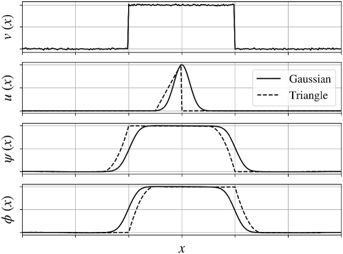
One can think of convolution and cross-correlation as weighting operations (with weighting function defined by the operator). The weighting function can be designed in different ways to perform different operations to the signal such as averaging, smoothing, differentiation, and pattern recognition. In Figure 1 we illustrate the application of a Gaussian operator to a noisy rectangular signal . We note that the convolved and cross-correlated signals are identical (because the operator is symmetric and thus ). We also note that the output signals are smooth versions of the input signal; this is because a Gaussian operator has the effect of extracting frequencies from the signal (a fact that can be established from Fourier analysis). Specifically, we recall that the Fourier transform of the convolved signal satisfies:
| (2) |
where is the Fourier transform of scalar function . Here, the product has the effect of preserving the frequencies in the signal that are also present in the operator . In other words, convolution acts as a filter of frequencies; as such, one often refers to operators as filters. By comparing the output signals of convolution and cross-correlation obtained with the triangular operator, we can confirm that one is the mirror version of the other. From Figure 1, we also see that the output signals are smooth variants of the input signal; this is because the triangular operator also extracts frequencies from the input signal (but the extraction is not as clean as that obtained with the Gaussian operator). This highlights the fact that different operators have different frequency content (known as the frequency spectrum).
Convolution and cross-correlation are implemented computationally by using discrete representations; these signals are represented by column vectors and with entries denoted as , , (note that ). Here, we note that the input and operator are defined over a 1D grid. The discrete convolution results in vector with entries given by:
| (3) |
Here, we use to denote the integer sequence . We note that computing at a given location requires operations and thus computing the entire output signal (spanning ) requires operations; consequently, convolution becomes expensive when the signal and operator are long vectors; as such, the operator is often a vector of low dimension (compared to the dimension of the signal ). Specifically, consider the operator with entries (thus ) and assume (typically ). The convolution is given by:
| (4) |
This reduces the number of operations needed from to .
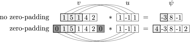
The convolved signal is obtained by using a moving window starting at the boundary and by moving forward as until reaching . We note that the convolution is not properly defined close to the boundaries (because the window lies outside the domain of the signal). This situation can be remedied by starting the convolution at an inner entry of such that the full window is within the signal (this gives a proper convolution). However, this approach has the effect of returning a signal that is smaller than the original signal . This issue can be overcome by artificially padding the signal by adding zero entries (i.e., adding ghost entries to the signal at the boundaries). This is an improper convolution but returns a signal that has the same dimension as (this is often convenient for analysis and computation). Figure 2 illustrates the difference between convolutions with and without padding. We also highlight that it is possible to advance the moving window by multiple entries as (here, is known as the stride). This has the effect of reducing the number of operations (by skipping some entries in the signal) but returns a signal that is smaller than the original one.
By defining signals and with entries and , one can also express the valid convolution operation in an asymmetric form as:
| (5) |
In CNNs, one often applies multiple operators to a single input signal or one analyzes input signals that have multiple channels. This gives rise to the concepts of single-input single-output (SISO), single-input multi-output (SIMO), and multi-input multi-output (MIMO) convolutions.
In SISO convolution, we take a 1-channel input vector and output a vector (a 1-channel signal), as in (5). In SIMO convolution, one uses a single input and a collection of operators with . Here, every element is an -dimensional vector and we represent the collection as the object . SIMO convolution yields a collection of convolved signals with and with entries given by:
| (6) |
In MIMO convolution, we consider a multi-channel input given by the collection ( is the number of channels); the collection is represented as the object . We also consider a collection of operators with and ; in other words, we have operators per input channel and we represent the collection as the object . MIMO convolution yields the collection of convolved signals with and with entries given by:
| (7) | ||||
We see that, in MIMO convolution, we add the contribution of all channels to obtain the output object , which contains channels given by vectors of dimension . Channel combination loses information but saves computer memory.
2.2 2D Convolution Operations
Convolution and cross-correlation operations in 2D are analogous to those in 1D; the convolution and cross-correlation of a continuous operator and an input signal are denoted as and and are given by:
| (8a) | ||||
| (8b) | ||||
As in the 1D case, the terms convolution and cross-correlation are used interchangeably; here, we will use the cross-correlation form (typically used in CNNs).
In the discrete case, the input signal and the convolution operator are matrices and with entries and (thus and ). For simplicity, we assume that these are square matrices and we note that the input and operator are defined over a 2D grid. The convolution of the input and operator matrices results in a matrix with entries:
| (9) |
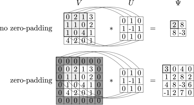
In Figure 3 we illustrate 2D convolutions with and without padding. The 2D convolution (in valid and asymmetric form) can be expressed as:
| (10) |
where , and .
The SISO convolution of an input and an operator is given by (10) and outputs a matrix . In SIMO convolution, we are given a collection of operators with . A convolved matrix is obtained by applying the -th operator to the input :
| (11) |
for . The collection of convolved matrices is represented as object .
In MIMO convolution, we are given a -channel input collection with and represented as . We convolve this input with the operator object , which is a collection . This results in an object given by the collection for and with entries given by:
| (12) | ||||
for , and . For convenience, the input object is often represented as a 3D tensor , the convolution operator is represented as the 4D tensor , and the output signal is represented as the 3D tensor . We note that, if and (1-channel inputs and channels), these tensors become matrices. Tensors are high-dimensional quantities that require significant computer memory to store and significant power to process.
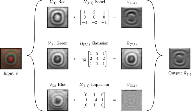
MIMO convolutions in 2D are typically used to process RGB images (3-channel input), as shown in Figure 4. Here, the RGB image is the object and each input channel is a matrix; each of these matrices is convolved with an operator . Here we assume (one operator per channel). The collection of convolved matrices are combined to obtain a single matrix . If we consider a collection of operators with , and , the output of MIMO convolution returns the collection of matrices with , which is assembled in the tensor . Convolution with multiple operators allows for the extraction of different types of features from different channels.
We highlight that the use of channels is not restricted to images; specifically, channels can be used to input data of different variables in a grid (e.g., temperature, concentration, density). As such, channels provide a flexible framework to express multivariate data.
We also highlight that a grayscale image is a 1-channel input matrix (the RGB channels are combined in a single channel). In a grayscale image, every pixel (an entry in the associated matrix) has a certain light intensity value; whiter pixels have higher intensity and darker pixels have a lower intensity (or the other way around). The resolution of the image is dictated by the number of pixels and thus dictates the size of the matrix; the size of the matrix dictates the amount of memory needed for storage and computations needed for convolution. It is also important to emphasize that any matrix can be visualized as a grayscale image (and any grayscale image has an underlying matrix). This duality is important because visualizing large matrices (e.g., to identify patterns) is difficult if one directly inspects the numerical values; as such, a convenient approach to analyze patterns in large matrices consists of visualizing them as images.
Finally, we highlight that convolution operators can be applied to any grid data object in higher dimensions (e.g., 3D and 4D) in a similar manner. Convolutions in 3D can be used to process video data (each time frame is an image). However, 3D data objects can also be used to represent data distributed over 3D Euclidean spaces (e.g., density or flow in a 3D domain). However, the complexity of convolution operations in 3D (and higher dimensions) is substantial. In the discussion that follows we focus our attention to 2D convolutions; in Section 6 we illustrate the use of 3D convolutions in a practical application.
3 Convolution Operators
Convolution operators are the key functional units that a CNN uses to extract features from input data objects. Some commonly used operators and their transformation effect are shown in Figure 4. When the input is convolved with a Sobel operator, the output highlights the edges (gradients of intensity). The reason for this is that the Sobel operator is a differential operator. To explain this concept, consider a discrete 1D signal ; its derivative at entry can be computed using the finite difference:
| (13) |
This indicates that we can compute the derivative signal by applying a convolution of the form with operator . Here, the operator can be scaled as as this does not alter the nature of the operation performed (just changes the scale of the entries of ).
The Sobel operator shown in Figure 4 is a matrix of the form:
| (14) |
where the vector approximates the first derivative in the vertical direction, and is a binomial operator that smooths the input matrix.
Another operator commonly used to detect edges in images is the Laplacian operator; this operator is an approximation of the continuous Laplacian operator . The convolution of a matrix using a Laplacian operator is:
| (15) |
This reveals that the convolution is an approximation of that uses a 2D finite difference scheme; this scheme has an operator of the form:
| (16) |
The transformation effect of the Laplacian operator is shown in Figure 4. In the partial differential equations (PDE) literature, the non-zero structure of a finite-difference operator is known as the stencil [33]. As expected, a wide range of finite difference approximations (and corresponding operators) can be envisioned. Importantly, since the Laplacian operator computes the second derivative of the input, this is suitable to detect locations of minimum or maximum intensity in an image (e.g., peaks). This allows us to understand the geometry of matrices (e.g., geometry of images or 2D fields). Moreover, this also reveals connections between PDEs and convolution operations.
The Gaussian operator is commonly used to smooth out images. A Gaussian operator is defined by the density function:
| (17) |
where is the standard deviation. The standard deviation determines the spread of of the operator and is used to control the frequencies removed from a signal. We recall that the density of a Gaussian is maximum at the center point and decays exponentially (and symmetrically) when moving away from the center. Discrete representations of the Gaussian operator are obtained by manipulating and truncating the density in a window. For instance, the Gaussian operator as shown in Figure 4 is:
| (18) |
Here, we can see that the operator is square and symmetric, has a maximum value at the center point, and the values decay rapidly as one moves away from the center.
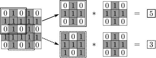
Convolution operators can also be designed to perform pattern recognition; for instance, consider the situation in which you want to highlight areas in a matrix that have a pattern (feature) of interest. Here, the structure of the operator dictates the 0-1 pattern sought. For instance, in Figure 5 we present an input matrix with 0-1 entries and we perform a convolution with an operator with a pre-defined 0-1 structure. The convolution highlights the areas in the input matrix in which the presence of the sought pattern is strongest (or weakest). As one can imagine, a huge number of operators could be designed to extract different patterns (including smoothing and differentiation operators); moreover, in many cases it is not obvious which patterns or features might be present in the image. This indicates that one requires a systematic approach to automatically determine which features of an input signal (and associated operators) are most relevant.
4 CNN Architectures
CNNs are hierarchical (layered) models that perform a sequence of convolution, activation, pooling, flattening operations to extract features from input data object. The output of this sequence of transformation operations is a vector that summarizes the feature information of the input; this feature vector is fed to a fully-connected neural net that makes final predictions. The goal of the CNN is to determine the features of a set of input data objects (input data samples) that best predict the corresponding output samples. Specifically, the input of the CNN are a set of sample objects with sample index , and the output of the CNN are the corresponding predicted labels . The goal of a CNN is to determine convolution operators giving features that best match the predicted labels to the output labels; in other words, the CNN seeks to find operators (and associated features) that best map the inputs to the outputs.
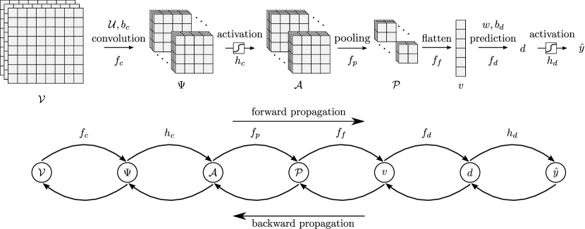
In this section we discuss the different elements of a 2D CNN architecture. To facilitate the analysis, we construct a simple CNN of the form shown in Figure 6. This architecture contains a single layer that performs convolution, activation, pooling, and flattening. Generalizing the discussion to multiple layers and higher dimensions (e.g., 3D) is rather straightforward once the basic concepts are established. Also, in the discussion that follows, we consider a single input data sample (that we denote as ) and discuss the different transformation operations performed to it along the CNN to obtain a final prediction (that we denote as ). We then discuss how to combine multiple samples to train the CNN. We emphasize that our goal here is to focus on the foundations of CNNs; discussing more complex architectures (e.g., with more layers or multiple outputs) requires introducing additional notation and concepts that we believe will blur our main message.
4.1 Convolution Block
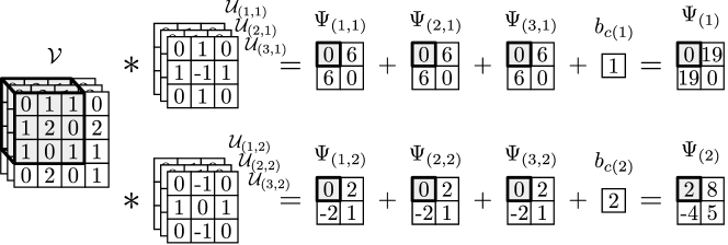
An input sample of the CNN is the tensor . The convolution block uses the operator to conduct a MIMO convolution. The output of this convolution is the tensor with entries given by:
| (19) |
where , , and . A bias parameter is added after the convolution operation; the bias helps adjust the magnitude of the convolved signal. To enable compact notation, we define the convolution block using the mapping ; here, we note that the mapping depends on the parameters (the operators) and (the bias). An example of a convolution block with a 3-channel input and 2-channel operator is shown in Figure 7.
4.2 Activation Block
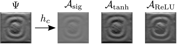
The convolution block outputs the signal ; this is passed through an activation block given by the mapping with . Here, we define an activation mapping of the form . The activation of is conducted element-wise as:
| (20) |
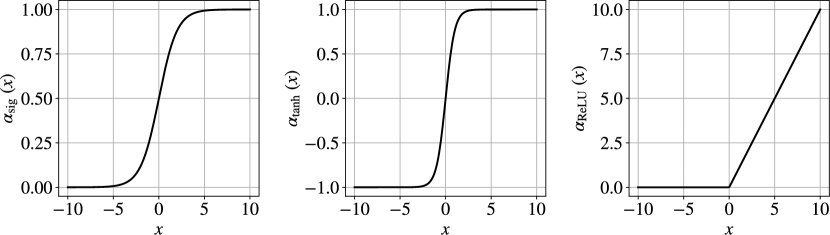
where is an activation function (a scalar function). Typical activation functions include the sigmoid, hyperbolic tangent (tanh), and Rectified Linear Unit (ReLU):
| (21) | ||||
Figures 8 and 9 illustrate the transformation induced by the activation functions. These functions act as basis functions that, when combined in the CNN, enable capturing nonlinear behavior. A common problem with sigmoid and tanh functions is that they exhibit the so-called vanishing gradient effect [11]. Specifically, when the input values are large or small in magnitude, the gradient of the sigmoid and tanh functions is small (flat at both ends) and this makes the activation output insensitive to changes in the input. Furthermore, both the sigmoid and tanh functions are sensitive to the change in input when the output is close to 1/2 and zero, respectively. The ReLU function is commonly used to avoid vanishing gradient effects and to increase sensitivity [26]. This activation function outputs a value of zero when the input is less than or equal to zero, but outputs the input value itself when the input is greater than zero. The function is linear when the input is greater than zero, which makes the CNN easier to optimize with gradient-based methods [11]. However, ReLU is not continuously differentiable when the input is zero; in practice, CNN implementations assume that the gradient is zero when the input is zero.
4.3 Pooling Block
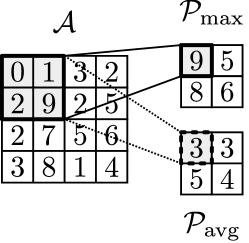
The pooling block is a transformation that reduces the size of the output obtained by convolution and subsequent activation. This block also seeks to make the representation approximately invariant to small translation of the inputs [11]. Max-pooling and average-pooling are the most common pooling operations (here we focus on max-pooling). The pooling operation can be expressed as a mapping and delivers a tensor . To simplify the discussion, we denote ; the max-pooling operation with is defined as:
| (22) |
where , . In Figure 10, we illustrate the max-pooling and averaging pooling operations on a 1-channel input.
Operations of convolution, activation, and pooling constitute a convolution unit and deliver an output object . This object can be fed into another convolution unit to obtain a new output object and this recursion can be performed over multiple units. The recursion has the effect of highlighting different features of the input data object (e.g., that capture local and global patterns). In our discussion we consider a single convolution unit.
4.4 Flattening Block
The convolution, activation, and pooling blocks deliver a tensor that is flattened to a vector (with some abuse of notation where was originally defined for input signal in 1D); this vector is fed into a fully-connected (dense) block that performs the final prediction. The vector is typically known as the feature vector. The flattening block is represented as the mapping with that outputs . Note that this block is simply a vectorization of a tensor.
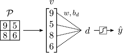
4.5 Prediction (Dense) Block
The feature vector is input into a prediction block that delivers the final prediction . This block is typically a fully-connected (dense) neural net with multiple weighting and activation units (here we only consider a single unit). The prediction block first mixes the elements of the feature vector as:
| (23) |
where is the weighting (parameter) vector and is the bias parameter. The scalar is normally known as the evidence. We denote the weighting operation using the mapping and thus . In Figure 11, we illustrate this weighting operation. An activation function is applied to the evidence to obtain the final prediction with . This involves an activation (e.g., with a sigmoidal or ReLU function). We thus have that the prediction block has the form . One can build a multi-layer fully-connected network by using a recursion of weighting and activation steps (here we consider one layer to simplify the exposition). Here, we assume that the CNN delivers a single (scalar) output . In practice, however, a CNN can also predict multiple outputs; in such a case, the weight parameter becomes a matrix and the bias is a vector. We also highlight that the predicted output can be an integer value (to perform classification tasks) or a continuous value (to perform regression tasks).
5 CNN Training
CNN training aims to determine the parameters (operators and biases) that best map the input data to the output data. The fundamental operations in CNN training are forward and backward propagation, which are used by an optimization algorithm to improve parameters. In forward propagation, the input data is propagated forward through the CNN (block by block and layer by layer) to make a prediction and evaluate a loss function that captures the mismatch between the predicted and true output. In backward propagation, one computes the gradient of the loss function with respect to each parameter via a recursive application of the chain rule of differentiation (block by block layer by layer). This recursion starts in the prediction block and proceeds backwards to the convolution block. Notably, we will see that the derivatives of the transformation blocks have explicit (analytical) representations.
5.1 Forward Propagation
To explain the process of forward propagation, we consider the CNN architecture shown in Figure 6 with an input and an output (prediction) . All parameters , , and are flattened and concatenated to form a parameter vector , where . We can express the entire sequence of operations carried out in the CNN as a composite mapping and thus . We call this mapping the forward propagation mapping (shown in Figure 6) and note that this can be decomposed sequentially (via lifting) as:
| (24) | ||||
This reveals the nested nature and the order of the CNN transformations on the input data. Specifically, we see that one conducts convolution, activation, pooling, flattening, and prediction.
To perform training, we collect a set of input samples and corresponding output labels with sample index . Our aim is to compare the true output labels to the CNN predictions . To do so, we define the loss function that we aim to minimize. For classification tasks, the output is binary and a common loss function is the cross-entropy [17]:
| (25) |
For regression tasks, we have that the output is continuous and a common loss function is the mean squared error:
| (26) |
In compact form, we can write the loss function as . Here, contains all the input samples for . The loss function can be decomposed into individual samples and thus we can express it as:
| (27) |
where is the contribution associated with the -th data sample.
5.2 Optimization Algorithms
The parameters of the CNN are obtained by finding a solution to the optimization problem:
| (28) |
The loss function embeds the forward propagation mapping (which is a highly nonlinear mapping); as such, the loss function might contain many local minima (and such minima tend to be flat [12]). We recall that appearance of flat minima is often the manifestation of model overparameterization; this is due to the fact that the parameter vector can contain hundreds of thousands to millions of values. As such, training of CNNs need to be equipped with appropriate validation procedures (to ensure that the model generalizes well). Most optimization algorithms used for CNNs are gradient-based (first-order); this is because second-order optimization methods (e.g., Newton-based) involve calculating the Hessian of the loss function with respect to parameter vector , which is computationally expensive (or intractable). Quasi-Newton methods (e.g., limited-memory BFGS) are also often used to train CNNs.
Gradient descent (GD) is the most commonly used algorithm to train CNNs. This algorithm updates the parameters as:
| (29) |
where is the learning rate (step length) and is the step direction. In GD, the step direction is set to (the gradient of the loss). Since the loss function is a sum over samples, the gradient can be decomposed as:
| (30) |
Although GD is easy to compute and implement, is not updated until the gradient of the entire dataset is calculated (which can contain millions of data samples). In other words, the parameters are not updated until all the gradient components are available. This leads to load-imbalancing issues and limits the parallel scalability of the algorithm.
Stochastic gradient descent (SGD) is a variant of GD that updates more frequently (with gradients from a partial number of samples). Specifically, changes after calculating the loss for each sample. SGD updates the parameters by using the step , where sample is selected at random. Since is updated frequently, SGD requires less memory and has better parallel scalability [20]. Moreover, it has been shown empirically that this algorithm has the tendency to escape local minima (it explores the parameter space better). However, if the training sample has high variance, SGD will converge slowly.
Mini-batch GD is an enhancement of SGD; here, the entire dataset is divided into batches and is updated after calculating the gradient of each batch. This results in a step direction of the form:
| (31) |
where is a set of sample corresponding to batch and the entries of the batches are selected at random. Mini-batch GD updates the model parameters frequently and has faster convergence in the presence of high variance [41].
5.3 Backward Propagation
Backward propagation (backpropagation) seeks to compute elements of the gradient of the loss by recursive use of the chain rule. This approach exploits the nested nature of the forward propagation mapping:
| (32) |
This mapping can be expressed in backward form as:
| (33a) | ||||
| (33b) | ||||
| (33c) | ||||
| (33d) | ||||
| (33e) | ||||
| (33f) | ||||
An illustration of this backward sequence is presented in Figure 6. Exploiting this structure is essential to enable scalability (particularly for saving memory). To facilitate the explanation, we consider the squared error loss defined for a single sample (generalization to multiple samples is trivial due to the additive nature of the loss):
| (34) |
Our goal is to compute the gradient (the parameter step direction) ; here, we have that parameter .
Prediction Block Update.
The step direction for the parameters (the gradient) in the prediction block is defined as and its entries are given by:
| (35) | ||||
with . If we define then we can establish that the update has the simple form and thus:
| (36) |
The gradient for the bias is given by:
| (37) | ||||
and thus:
| (38) |
Convolutional Block.
An important feature of CNN is that some of its parameters (the convolution operators) are tensors and we thus require to compute gradients with respect tensors. While this sounds complicated, the gradient of the convolution operator has a remarkably intuitive structure (provided by the grid nature of the data and the structure of the convolution operation). To see this, we begin the recursion at:
| (39) |
Before computing , we first obtain the gradient for the feature vector as:
| (40) | ||||
with and thus:
| (41) |
If we define the inverse mapping of the flattening operation as , we can express the update of the pooling block as:
| (42) |
The gradient from the pooling block is passed to the activation block via up-sampling. If we have applied max-pooling with a pooling operator, then:
| (43) |
where calculates the remainder obtained after dividing by .
The gradient with respect to the convolution operator has entries of the form:
| (44) | ||||
for and , and with:
| (45) | ||||
If we define , then:
| (46) |
The gradient with respect to the bias parameters in the convolution block has entries:
| (47) | ||||
with . Because , and
| (48) | ||||
we have that:
| (49) |
5.4 Saliency Maps
Saliency maps is a useful technique used to determine features that best explain a prediction; in other words, these techniques seek to highlight what the CNN searches for in the data. The most basic version of the saliency map is based on gradient information for the loss (with respect to the input data) [34]. Recall that the forward propagation function is given by , where the input is , and the parameter vector is . We express the loss function as (for input sample ); the saliency map is a tensor of the same dimension as the input and is given by:
| (50) |
If we are only interested in the location of the most important regions, we can take the maximum value of over all channels and generate the saliency mask (a matrix). In some cases, we can also study the saliency map for each channel, as this may have physical significance. Saliency maps are easy to implement (can be obtained via back-propagation) but suffer from vanishing gradients effects. The so-called integrated gradient (IG) seeks to overcome vanishing gradient effects [38]; the IG is defined as:
| (51) |
where is a baseline input that represents the absence of a feature in the input . Typically, is a sparse object (few non-zero entries).
6 Applications
CNNs have been applied to different problems arising in chemical engineering (and related fields) but have been applied mostly to image data. In this section, we present different case studies to highlight the broad versatility of CNNs; specifically, we show how to use CNNs to make predictions from grid data objects that are general vectors (in 1D), matrices (in 2D), and tensors (in 3D). Our discussion also seeks to highlight the different concepts discussed. The scripts to reproduce the results for the optimal control (1D), the multivariate process monitoring (2D) and the molecular simulations (3D) case studies can be found here https://github.com/zavalab/ML/tree/master/ConvNet.
6.1 Optimal Control (1D)
Optimal control problems (OCP) are optimization problems that are commonly encountered in engineering. The basic idea is to find a control trajectory that drives a dynamical system in some optimal sense. A common goal, for instance, is to find a control trajectory that minimizes the distance of the system state to a given reference trajectory. Here, we study nonlinear OCPs for a quadrotor system [14]. In this problem, we have an inverted pendulum that is placed on a quadrotor, which is required to fly along a reference trajectory. The governing equations of the quadrotor-pendulum system are:
| (52) | ||||
where are the positions and are angles. We define as state variables, where are velocities. The control variables are , where is the vertical acceleration and are the angular velocities of the quadrotor fans. Our goal is to find a control trajectory that minimizes the cost:
| (53) |
where is a time-varying reference trajectory (changes every 30 seconds) and is assumed to be zero. Minimization of this cost seeks to keep the quadrotor trajectory close to the reference trajectory with as little control action (energy) as possible. An example reference trajectory is shown in Figure 12; here, we show the reference trajectories for and and the trajectories for the rest of the states are assumed to be zero.
In this case study, we want to train a 1D CNN to predict optimal cost values based on a given reference trajectory for the states (without the need of solving the OCP). This type of capability can be used to determine reference trajectories that are least/most impactful on performance (i.e., trajectories that are difficult or easy to track). CNNs can also be used to approximate optimal control laws, which can significantly reduce online computational time and enable fast model predictive control implementations. To train the CNN, we generated 200 random trajectories and solved the corresponding OCPs. Each OCP was discretized, modeled with JuMP [8], and solved with IPOPT [40] [1]. After solving each OCP, we obtained the optimal states and controls and (shown in Figure 12) and the optimal cost .
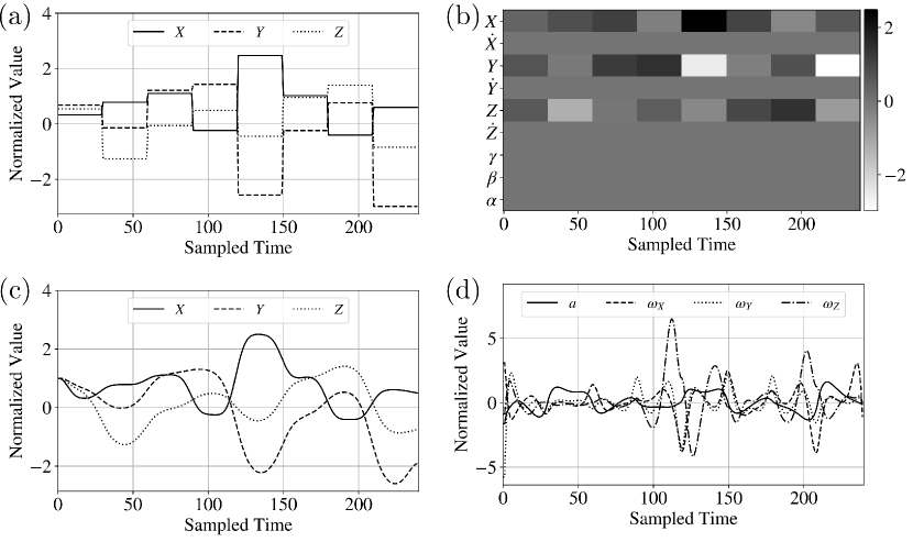
The cost is the output of the 1D CNN; to obtain the input, we need to represent the reference trajectory (which includes multiple state variables) as a 1D grid object that the CNN can analyze. Here, we represent as a multi-channel 1D grid object. The data object is denoted as ; this object has channels and each channel is a vector of dimension (each channel contains the trajectory of one of the state variables).We visualize this multi-channel object as a grayscale image (each row is channel), see Figure 12. We can see that this representation provides a different perspective on the nature of the reference trajectories (in the form of patterns). The goal is to train the 1D CNN to recognize how features of such patterns impact cost (e.g., abrupt vs. mild changes in the reference trajectory). We note that the data object could, in principle, be represented as a single-channel matrix that could be fed to a 2D CNN. However, this approach would require 2D convolution operations (as opposed to the cheaper 1D convolutions). The results presented here seek to highlight that a 1D CNN suffices and gives accurate predictions. This also seeks to highlight the versatility that one has in representing data objects in different forms.
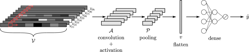
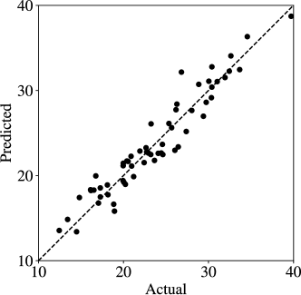
The training:validation:testing data ratio used is 3:1:2. The 1D CNN architecture is of the form Conv(64)-MaxPool-Flatten-Dense(32)-Dense(32), where the number in the parentheses is either the number of convolution operators or dense layer units. The architecture is shown in Figure 13; here, we can see that we have a single convolution unit but the prediction block has a couple of layers. The final prediction block generates a scalar prediction (corresponding to the cost). Regression results for the 1D CNN are presented in Figure 14; we can see that accurate predictions can be obtained. Compared with a feed-forward neural net (RMSE=5.44) and a linear regression (RMSE=8.56), the 1D CNN has a more accurate prediction. This performance is quite surprising given the complex nature of the reference trajectories and the nonlinearity of the system. Specifically, the 1D CNN has learned to recognize patterns that have the strongest effect on cost.
6.2 Flow Cytometry (2D)
This case study is based on the results presented in [19]; our goal here is not to revisit these results; instead, we seek to highlight the data representation aspects of the problem (how to start from raw data into an input representation that the CNN can process).
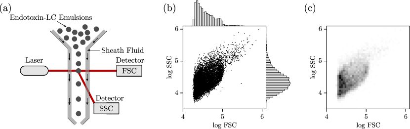
Endotoxins are lipopolysaccharides (LPS) present in the outer membrane of gram-negative bacteria; these agents are responsible for the pathophysiological phenomena associated with gram-negative infections, such as endotoxemia (septic shock caused by a severe immune response) [24]. It has been recently discovered that micrometer-sized liquid crystal (LC) droplets dispersed in an aqueous solution can be used as a sensing method to detect and measure the concentration of endotoxins of different bacterial organisms. After exposure to endotoxins, LC droplets undergo ordering transitions that yield distinct optical properties and this change can be detected using flow cytometry (as shown in Figure 15). Flow cytometry produces scatter point clouds of forward and side scattering (FSC/SSC) as shown in Figure 15 (each point represents a scattering event of a given droplet). A point could be converted into a 2D grid data object via binning; this is done by discretizing the FSC/SSC domain and by counting the number of points in a bin. The 2D grid object obtained is a matrix that we visualize as a grayscale image; here, each pixel is a bin and the intensity is the number of events in the bin (bins with more events appear darker). We note that this visualization is a 2D projection of a 3D histogram (the third dimension corresponds to the number of events, also known as the frequency). In other words, the 2D grid object captures the geometry (shape) of the joint probability density of the FSC/SSC. This shape has curvature and this can be characterized by gradients (derivatives).
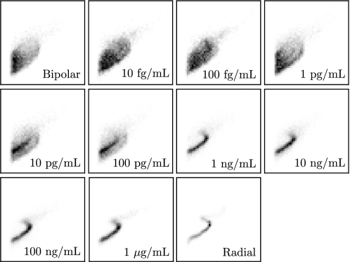
The effect of endotoxin concentration on the FSC/SSC scatter fields (after binning) is shown in Figure 16; clear differences in the patterns can be observed at concentrations that are far apart but difference are subtle for nearby concentrations. Our goal is to train a 2D CNN that can predict concentrations from the scatter fields.
We used the following procedure to obtain the 2D grid data objects (samples) that were fed to the CNN. For each sample, we generated bins for a given scatter field by partitioning the FSC and SSC dimensions into 50 segments (the grid has pixels). For each sample, we were also given reference scatter fields that represented limiting behavior: bipolar control (negative) and radial control (positive). Each sample is given by a 3-channel object where the first channel is the negative reference matrix , the second channel is the target matrix , and the third channel is a positive reference matrix (each channel contains a matrix). This procedure is illustrated in Figure 17. This multi-channel data representation approach has been found to magnify differences in the target matrix from the references (we will see that neglecting the negative/positive references does not give accurate predictions). The data representation used highlights how multi-channel inputs can be used in creative ways to encode different properties of the data at hand.
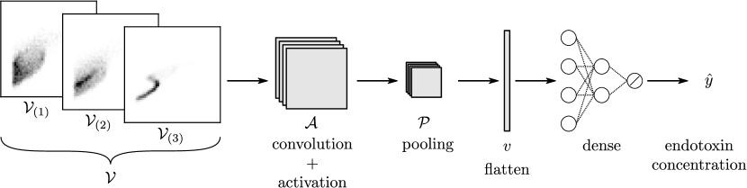
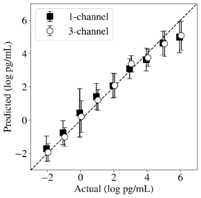
The 3-channel data object was fed to a CNN, which we call EndoNet. EndoNet has an architecture of Conv(64)-MaxPool-Flatten-Dense(32)-Dense(32)-Dense(1). The output block generates a scalar prediction (corresponding to the endotoxin concentration). In other words, the CNN seeks to predict the endotoxin concentration from the input flow cytometry fields. The architecture of EndoNet is shown in Figure 17. The regression results for EndoNet are presented in Figure 18. EndoNet can extract pattern information within and between each channel of the input image (which include negative and positive controls). Capturing differences between channels provides context for the CNN and has the effect of highlighting the domains in the scatter field that contain the most information. To validate this hypothesis, we conducted predictions for EndoNet using only the 1-channel representation as input (we ignored the positive and negative channels). For the 1-channel data representation we obtained an RMSE of 0.97; for the 3-channel representation we obtained and RMSE of 0.78. It is particularly remarkable that EndoNet can accurately predict concentrations that span eight orders of magnitude.
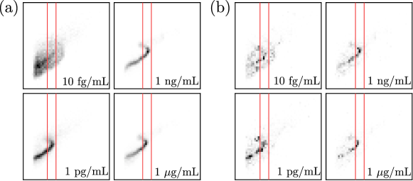
We use saliency maps to highlight features that EndoNet is searching for to make predictions. The saliency map used is calculated by integrated gradients; here the map is a matrix . Figure 19 presents saliency maps obtained with EndoNet; here, we notice several important emerging patterns. First, the saliency maps clusters around a characteristic S-region used in traditional counting methods (the region between the red lines) [25]. This indicates that EndoNet searches for information in the same region as this traditional method; however, the saliency maps also indicate that there is a clear diagonal pattern that must be considered. The saliency maps also reveal regions that do not provide information for classification and regression. Specifically, we see that regions of high FSC and SSC values do not provide significant information.
6.3 Multivariate Process Monitoring (2D)
Fault detection is a common task performed in process monitoring. Here, the idea is to collect multivariate time series (for different process variables) under different modes of operation (each mode is induced by a specific fault). The goal is to identify features (signatures) in the time series to determine if the process is a given mode. We focus on a case study for the Tennessee-Eastman (TE) process [7]. We expand the recent work presented in [42], which shows that multivariate signals can be processed as matrices and used by CNNs to identify faults. This work is expanded by performing CNN architecture optimization and by performing saliency map analysis to identify critical variables that best explain faults.
The TE process units include a reactor, condenser, compressor, separator and stripper. The TE process produces two products (G and H) and a byproduct (F) from four reactants (A, C, D and E). Component B is an inert compound. In total, the TE process contains a total of 52 measured variables; 41 of them are process variables and 11 are manipulated variables. This process exhibits 20 different types of faults, as listed in Table 1.
[t] Fault ID Fault Name Type Fault 1 A/C feed ratio, B composition constant (stream 4) Step Fault 2 B composition, A/C ratio constant (stream 4) Step Fault 3 D feed temperature (stream 2) Step Fault 4 Reactor cooling water inlet temperature Step Fault 5 Condenser cooling water inlet temperature Step Fault 6 A feed loss (stream 1) Step Fault 7 C header pressure loss - reduced availability (stream 4) Step Fault 8 A, B, C feed composition (stream 4) Random variation Fault 9 D feed temperature (stream 2) Random variation Fault 10 C feed temperature (stream 4) Random variation Fault 11 Reactor cooling water inlet temperature Random variation Fault 12 Condenser cooling water inlet temperature Random variation Fault 13 Reaction kinetics Slow drift Fault 14 Reactor cooling water valve Sticking Fault 15 Condenser cooling water valve Sticking Fault 16-20 Unknown Unknown
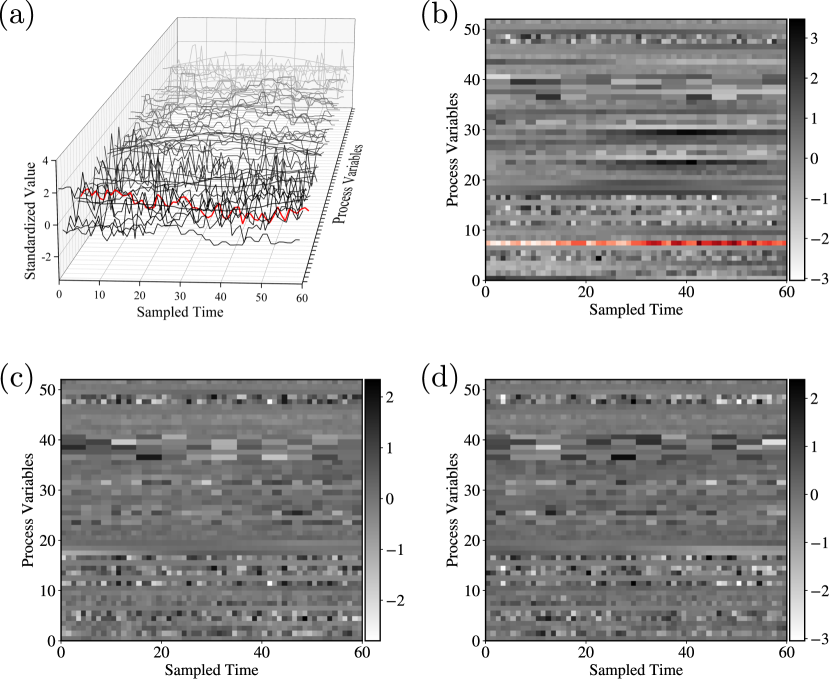
The TE process data is obtained from Harvard Dataverse [31]. The 52 process variables are sampled every 3 minutes. The transformation of multivariate signal data to matrices is shown in Figure 20. In the transformation, we construct an input data sample by using 52 signal vectors (each vector contains 60 time points) that are combined into matrix (). We have a total of 6947 input samples. The training:validation:testing data ratio used is 11:4:5. The model architecture is Conv(64)-MaxPool-Conv(64)-MaxPool-Flatten-Dense(128)-Dense(64)-Dense(20).
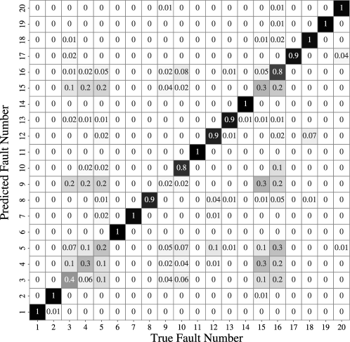
The confusion matrix is a visualization of performance in classification models. Each row of the confusion matrix represents instances of the predicted class and each column represents instances of the true class. The entries along the diagonal lines are where the instances are correctly classified. Figure 21 is a confusion matrix with an accuracy of 0.7561. With the exception of faults 3, 4, 5, 9, and 15, most faults can be identified accurately. Fault 3, 9 and 15 are especially difficult to detect because the mean, variance, and higher-order variances do not vary significantly [4, 45].
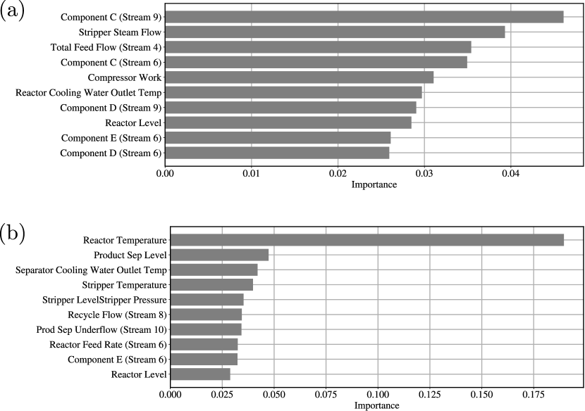
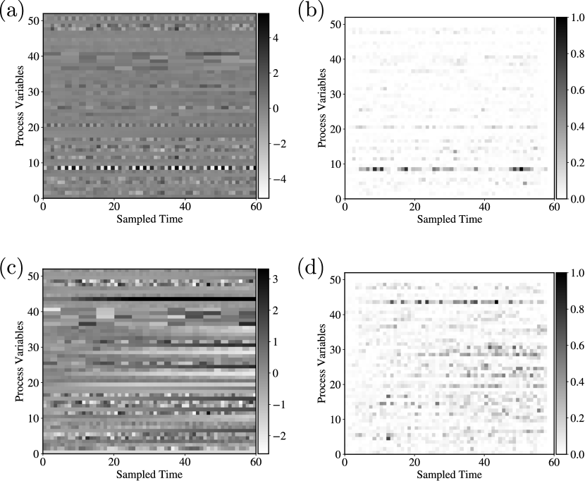
The saliency maps in this case study are calculated using integrated gradients; the maps are shown in Figure 22. The saliency maps reveal the most important TE process variables and time points for classification. We also performed saliency analysis for each fault. Specifically, we obtain the time-averaged saliency vector from the saliency map belonging to fault type . The -th entry represents the importance of the -th process variable in fault type . We sum all the saliency vectors that are in the same fault type and rank the most important among the 52 process variables. The results are shown in Figure 23; when the fault type is the random variation of A, B, C feed composition in stream 4, important variables are mostly related to the chemical composition in different streams (such as the compositions of component C, D, E in stream 6 and 9). This is because, in general, changes in the composition in one stream will affect the composition in another stream. When the fault type is the random variation of reactor cooling water inlet temperature, the most important variable is the reactor temperature. This is because the inlet temperature of the reactor cooling water directly affects the reactor temperature. We can thus see that saliency maps provide valuable information that facilitate interpretation of CNN predictions.
6.4 Molecular Simulations (3D)
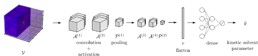
This case study is based on the 3D CNN reported in [3]. Our goal here is to focus on the data representation aspects of the problem in order to highlight how grid data can be used to represent 3D fields. Liquid-phase acid-catalyzed reactions can enhance biomass into high-value chemicals, but identifying the suitable solvent mixture that affects the reaction rate is challenging. In this case study, we want to show that the atomistic configuration of the reactant-solvent environment (containing reactant, water and cosolvent) generated by molecular dynamics (MD) simulations can be exploited by 3D CNNs to achieve accurate predictions of reaction rates.
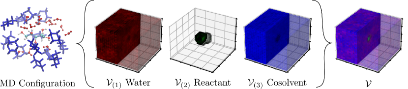
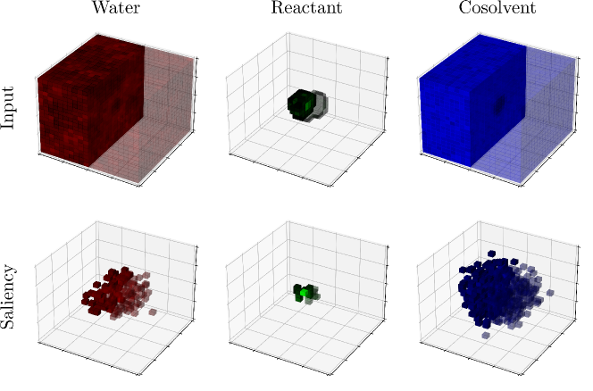
Figure 24 illustrates the data representation approach used to convert MD positions to a 3D tensor. For each MD configuration, we centered a 3D histogram on the center of mass of the reactant, which covered a cubic volume that was divided into a grid of bins (called voxels). For each bin, we calculated the water density by counting the number of water molecules within the bin and by normalizing. The same procedure was also performed to calculate the normalized occurrence of cosolvent and reactant oxygen atoms in each bin. The data object obtained for a single MD configuration is a 3-channel, 3D tensor. The first channel is the water density field, the second channel is the reactant field, and the third channel is the cosolvent field. The density field of each channel is a 3D tensor of dimension (each entry in a tensor is a voxel); this means that the 3D tensor is a projection of a 4D probability density function (three dimensions for space and the fourth dimension is the density value). This illustrates how tensors can be used to represent high-dimensional density functions and contain large amounts of information. We also observe that the data object can be treated as a 4D tensor of dimension . This data representation is illustrated in Figure 24. The goal here is to train a 3D CNN to identify features in the water, solvent, and cosolvent density fields that best explain reactivity. In other words, the CNN will learn to characterize the 3D solvent environment as we vary concentrations and types of reactants, solvents, and co-solvents. In total, we obtained 18240 tensors for 76 reaction-solvent systems.
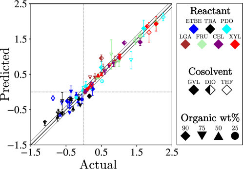
The 3-channel data object was fed to a 3D CNN, which we call SolventNet. The output block generates a scalar prediction (corresponding to the kinetic solvent parameter). The architecture of SolventNet is shown in Figure 25. Regression results for SolventNet are presented in Figure 26. The RMSE between actual and predicted values is 0.37, which is much better than the result (0.58) of previously reported methods. Specifically, SolventNet has good generality for various reactants, cosolvents and organic weight fractions, while the descriptor-based approach is ineffective in predicting systems with a large organic weight fraction.
The saliency map of SolventNet is calculated by integrated gradients. Examination of the saliency map in Figure 27 confirms that SolventNet primarily identifies features of the solvent environment within the local domain near the reactant. These plots clearly show that the region near the reactants is the most important for prediction, and that the size of the simulated volume is large enough that the region far from the reactants is not important.
7 Conclusions and Future Work
Convolutional neural networks (CNNs) are machine learning models that analyze grid-like data to unravel hidden patterns and features to make predictions. We have shown that data representations used by CNNs offer significant flexibility to tackle different types of applications (that go beyond computer vision). We have provided a review of key concepts behind CNNs (convolutions, multi-channel signals, operators, forward/backward propagations, and saliency maps) under a unifying mathematical framework. Our objective here is to establish connections with concepts from other mathematical fields and to highlight key computations that take place inside these powerful models.
There are several opportunities to extend CNNs from an algorithmic stand-point. We have seen that the parameters of CNNs are tensors and thus a huge number of parameters need to be optimized; as such, strategies for regularization can be envisioned. Specifically, one can envision optimizing operators with predefined structures. The connections between differential operators and convolutions are also interesting; here, one can envision developing architectures with fixed differential operators that are combined to learn structures of partial differential equations. Opportunities also exist for using CNNs in new applications. For instance, the ability of 1D CNNs to analyze sequences could be used to build dynamic models; currently, such models are being developed using fully-connected neural nets (but CNNs are more effective at capturing time dependencies). There is also potential in using CNNs to analyze space-time datasets; as those arising in computational fluid dynamics and other PDE applications. In this context, a key computational challenge is generalizing CNNs to 4D (while capturing high resolutions). One possibility could be the creation of hybrid CNN models that partition the input domain into subdomains of high resolution and that combine this with information of the full domain at low resolution.
While CNNs are capable of analyzing grid-like data, data in science and engineering can also appear in non-grid form (e.g. graphs). For example, bonds in molecules can be interpreted as edges in a graph, while atoms are nodes. Recently, graph neural networks (GNNs) have become very popular for analyzing graph-structured data. GNNs have been successfully used to predict molecular quantum properties [10], reactivity [6] and other chemical properties [44]. However, the full application potential of GNNs in chemical engineering has not been explored. In addition, it would be useful to establish fundamental connections between CNNs and GNNs; specifically, CNNs are special classes of GNNs. Understanding such connections can help unify these powerful modeling paradigms.
Acknowledgments
We acknowledge funding from the U.S. National Science Foundation (NSF) under BIGDATA grant IIS-1837812 and also acknowledge partial support from the NSF through the University of Wisconsin Materials Research Science and Engineering Center (DMR-1720415). We thank Prof. Nicholas Abbott for providing the endotoxin detection dataset and Prof. Reid Van Lehn for providing the molecular simulation dataset.
References
- [1] Jeff Bezanson, Alan Edelman, Stefan Karpinski, and Viral B Shah. Julia: A fresh approach to numerical computing. SIAM review, 59(1):65–98, 2017.
- [2] Joan Bruna and Stéphane Mallat. Invariant scattering convolution networks. IEEE transactions on pattern analysis and machine intelligence, 35(8):1872–1886, 2013.
- [3] Alex K Chew, Shengli Jiang, Weiqi Zhang, Victor M Zavala, and Reid C Van Lehn. Fast predictions of liquid-phase acid-catalyzed reaction rates using molecular dynamics simulations and convolutional neural networks. Chemical Science, 11(46):12464–12476, 2020.
- [4] Leo H Chiang, Evan L Russell, and Richard D Braatz. Fault detection and diagnosis in industrial systems. Springer Science & Business Media, 2000.
- [5] Nadav Cohen, Or Sharir, and Amnon Shashua. On the expressive power of deep learning: A tensor analysis. In Conference on Learning Theory, pages 698–728, 2016.
- [6] Connor W Coley, Wengong Jin, Luke Rogers, Timothy F Jamison, Tommi S Jaakkola, William H Green, Regina Barzilay, and Klavs F Jensen. A graph-convolutional neural network model for the prediction of chemical reactivity. Chemical science, 10(2):370–377, 2019.
- [7] James J Downs and Ernest F Vogel. A plant-wide industrial process control problem. Computers & chemical engineering, 17(3):245–255, 1993.
- [8] Iain Dunning, Joey Huchette, and Miles Lubin. Jump: A modeling language for mathematical optimization. SIAM Review, 59(2):295–320, 2017.
- [9] Kunihiko Fukushima. Neocognitron: A self-organizing neural network model for a mechanism of pattern recognition unaffected by shift in position. Biological cybernetics, 36(4):193–202, 1980.
- [10] Justin Gilmer, Samuel S Schoenholz, Patrick F Riley, Oriol Vinyals, and George E Dahl. Neural message passing for quantum chemistry. In International Conference on Machine Learning, pages 1263–1272. PMLR, 2017.
- [11] Ian Goodfellow, Yoshua Bengio, and Aaron Courville. Deep learning. MIT press, 2016.
- [12] Benjamin D Haeffele and René Vidal. Global optimality in neural network training. In Proceedings of the IEEE Conference on Computer Vision and Pattern Recognition, pages 7331–7339, 2017.
- [13] Kaiming He, Xiangyu Zhang, Shaoqing Ren, and Jian Sun. Deep residual learning for image recognition, 2015.
- [14] Markus Hehn and Raffaello D’Andrea. A flying inverted pendulum. In 2011 IEEE International Conference on Robotics and Automation, pages 763–770. IEEE, 2011.
- [15] Seongmin Heo and Jay H Lee. Fault detection and classification using artificial neural networks. IFAC-PapersOnLine, 51(18):470–475, 2018.
- [16] Maya Hirohara, Yutaka Saito, Yuki Koda, Kengo Sato, and Yasubumi Sakakibara. Convolutional neural network based on smiles representation of compounds for detecting chemical motif. BMC bioinformatics, 19(19):526, 2018.
- [17] Katarzyna Janocha and Wojciech Marian Czarnecki. On loss functions for deep neural networks in classification. arXiv preprint arXiv:1702.05659, 2017.
- [18] Shuiwang Ji, Wei Xu, Ming Yang, and Kai Yu. 3d convolutional neural networks for human action recognition. IEEE transactions on pattern analysis and machine intelligence, 35(1):221–231, 2012.
- [19] Shengli Jiang, JungHyun Noh, CHULSOON PARK, Alexander Smith, Nicholas L. Abbott, and Victor M Zavala. Using machine learning to identify and quantify endotoxins from different bacterial species using liquid crystal droplets. Analyst, pages –, 2021.
- [20] Janis Keuper and Franz-Josef Pfreundt. Asynchronous parallel stochastic gradient descent: A numeric core for scalable distributed machine learning algorithms. In Proceedings of the Workshop on Machine Learning in High-Performance Computing Environments, pages 1–11, 2015.
- [21] Alex Krizhevsky, Ilya Sutskever, and Geoffrey E Hinton. Imagenet classification with deep convolutional neural networks. In Advances in neural information processing systems, pages 1097–1105, 2012.
- [22] Yann Le Cun, Lionel D Jackel, Brian Boser, John S Denker, Henry P Graf, Isabelle Guyon, Don Henderson, Richard E Howard, and William Hubbard. Handwritten digit recognition: Applications of neural network chips and automatic learning. IEEE Communications Magazine, 27(11):41–46, 1989.
- [23] Jonathan Long, Evan Shelhamer, and Trevor Darrell. Fully convolutional networks for semantic segmentation. In Proceedings of the IEEE conference on computer vision and pattern recognition, pages 3431–3440, 2015.
- [24] PH Mäkelä, BAD Stocker, and ET Rietschel. Handbook of endotoxin. Handbook of Endotoxin, 1:59–137, 1984.
- [25] Daniel S Miller, Xiaoguang Wang, James Buchen, Oleg D Lavrentovich, and Nicholas L Abbott. Analysis of the internal configurations of droplets of liquid crystal using flow cytometry. Analytical chemistry, 85(21):10296–10303, 2013.
- [26] Vinod Nair and Geoffrey E Hinton. Rectified linear units improve restricted boltzmann machines. In Proceedings of the 27th international conference on machine learning (ICML-10), pages 807–814, 2010.
- [27] An On-device Deep Neural Network. for face detection, 2017.
- [28] John Nickolls, Ian Buck, Michael Garland, and Kevin Skadron. Scalable parallel programming with cuda. Queue, 6(2):40–53, 2008.
- [29] Adam Paszke, Sam Gross, Francisco Massa, Adam Lerer, James Bradbury, Gregory Chanan, Trevor Killeen, Zeming Lin, Natalia Gimelshein, Luca Antiga, Alban Desmaison, Andreas Kopf, Edward Yang, Zachary DeVito, Martin Raison, Alykhan Tejani, Sasank Chilamkurthy, Benoit Steiner, Lu Fang, Junjie Bai, and Soumith Chintala. Pytorch: An imperative style, high-performance deep learning library. In H. Wallach, H. Larochelle, A. Beygelzimer, F. d Alche-Buc, E. Fox, and R. Garnett, editors, Advances in Neural Information Processing Systems 32, pages 8024–8035. Curran Associates, Inc., 2019.
- [30] Shaoqing Ren, Kaiming He, Ross Girshick, and Jian Sun. Faster r-cnn: Towards real-time object detection with region proposal networks. In Advances in neural information processing systems, pages 91–99, 2015.
- [31] Cory A. Rieth, Ben D. Amsel, Randy Tran, and Maia B. Cook. Additional Tennessee Eastman Process Simulation Data for Anomaly Detection Evaluation, 2017.
- [32] Henry A Rowley, Shumeet Baluja, and Takeo Kanade. Neural network-based face detection. IEEE Transactions on pattern analysis and machine intelligence, 20(1):23–38, 1998.
- [33] T. Sauer. Numerical Analysis. Pearson, 2018.
- [34] Karen Simonyan, Andrea Vedaldi, and Andrew Zisserman. Deep inside convolutional networks: Visualising image classification models and saliency maps. arXiv preprint arXiv:1312.6034, 2013.
- [35] Karen Simonyan and Andrew Zisserman. Two-stream convolutional networks for action recognition in videos. In Advances in neural information processing systems, pages 568–576, 2014.
- [36] Karen Simonyan and Andrew Zisserman. Very deep convolutional networks for large-scale image recognition. arXiv preprint arXiv:1409.1556, 2014.
- [37] Alexander Smith, Nicholas L Abbott, and Victor M Zavala. Convolutional network analysis of optical micrographs. 2020.
- [38] Mukund Sundararajan, Ankur Taly, and Qiqi Yan. Axiomatic attribution for deep networks. In Proceedings of the 34th International Conference on Machine Learning-Volume 70, pages 3319–3328. JMLR. org, 2017.
- [39] Christian Szegedy, Wei Liu, Yangqing Jia, Pierre Sermanet, Scott Reed, Dragomir Anguelov, Dumitru Erhan, Vincent Vanhoucke, and Andrew Rabinovich. Going deeper with convolutions, 2014.
- [40] Andreas Wächter and Lorenz T Biegler. On the implementation of an interior-point filter line-search algorithm for large-scale nonlinear programming. Mathematical programming, 106(1):25–57, 2006.
- [41] Chong Wang, Xi Chen, Alexander J Smola, and Eric P Xing. Variance reduction for stochastic gradient optimization. Advances in Neural Information Processing Systems, 26:181–189, 2013.
- [42] Hao Wu and Jinsong Zhao. Deep convolutional neural network model based chemical process fault diagnosis. Computers & chemical engineering, 115:185–197, 2018.
- [43] Weidi Xie, J Alison Noble, and Andrew Zisserman. Microscopy cell counting and detection with fully convolutional regression networks. Computer methods in biomechanics and biomedical engineering: Imaging & Visualization, 6(3):283–292, 2018.
- [44] Kevin Yang, Kyle Swanson, Wengong Jin, Connor Coley, Philipp Eiden, Hua Gao, Angel Guzman-Perez, Timothy Hopper, Brian Kelley, Miriam Mathea, et al. Analyzing learned molecular representations for property prediction. Journal of chemical information and modeling, 59(8):3370–3388, 2019.
- [45] Yingwei Zhang. Enhanced statistical analysis of nonlinear processes using kpca, kica and svm. Chemical Engineering Science, 64(5):801–811, 2009.