Convexity and Aigner’s Conjectures
Abstract.
Markov numbers are integers that appear in triples which are solutions of a Diophantine equation, the so-called Markov cubic
A classical topic in number theory, these numbers are related to many areas of mathematics such as combinatorics, hyperbolic geometry, approximation theory and cluster algebras.
One can associate to each a positive rational number a Markov number in a natural way. We give a new unified proof of certain conjectures from Martin Aigner’s book, Markov’s Theorem and 100 Years of the Uniqueness Conjecture. Our proof relies on a relationship between Markov numbers and the lengths of closed simple geodesics on the punctured torus discovered by H. Cohn.
1. Introduction
The Markov numbers are the positive integer solutions of the Diophantine equation
Markov in the late 1800s showed that all these solutions could be given the structure of a binary tree. It became customary (and useful) to index the Markov numbers by the rationals in the interval which stand at the same place in the Stern–Brocot binary tree (see Figures 2 and 3). Frobenius’ conjecture asserts that each Markov number appears at most once in this tree. If this conjecture is true, then the obvious order of Markov numbers gives rise to a new strict order on the rationals.
1.1. Aigner’s Monotonicity Conjectures
Aigner [1] proposed three conjectures to better understand this order.
-
(1)
(The fixed numerator conjecture) Let and be positive integers such that and then
-
(2)
(The fixed denominator conjecture) Let and be positive integers such that and then
-
(3)
(The fixed sum conjecture) Let and be positive integers such that and then
The fixed numerator conjecture was proved in [8] using ideas from cluster algebra theory and snake graphs. Their proof relies on a connection between Christoffel paths and Markov numbers (see [2] for a discussion) which provides a formulation of Markov numbers as continuant polynomials. The proof is rather technical and introduces several interesting tools for studying paths in the Cayley graph of the monoid with the usual generators. In [9], the authors prove the fixed numerator conjecture by using ”transformations” on paths in the Cayley graph. We will show how these results can be deduced by considerations of convexity established in [7]. Our proof is represented visually in Figure 4.
1.2. Geometry of the Markov numbers
The question of counting for Markov triples, that is for estimating the size of the set of Markov triples for which the sup norm is less than , was first investigated by Gurwood in his thesis. He established an asymptotic formula using a correspondence between Markov and Farey trees. Somewhat later Zagier [10] obtained an improved error term. At the time of writing the best result is due to a Rivin and the author [7]:
for a numerical constant which has a geometric interpretation.
The method introduced in [7] differs from that of Gurwood and Zagier in that it relies on ideas of H. Cohn to interpret the question in terms of geometry of hyperbolic surfaces. In [4] Cohn shows that the Markov triple is, up to multiplication by 3, the image under the character map of the modular torus. Recall that the modular torus is the quotient of the upper half plane by , the commutator subgroup of , acting by Mobius transformations. Secondly, he shows that the permutations and the Vieta flips used to construct Markov’s binary tree are induced by automorphisms of the fundamental group of the torus and concludes that acts transitively on Markov triples. It is well known that if is a discrete faithful representation and a closed curve homotopic on the surface , then , the length of the closed geodesic homotopic to on the surface , can be computed from the trace using the relation
We note that the absolute value of the trace of an element of is well defined. Now identifying with the fundamental group of the modular torus Cohn shows that if is a Markov number then there exists a simple loop such that
so there is an explicit relation between Markov numbers and lengths of simple geodesics on the modular torus. In [7] the simple closed curves are embedded as a subset of primitive elements in the integer lattice and the length function is shown, using a simple geometric argument, to extend to a proper convex function . Thus the counting problem for Markov numbers can be settled by counting integer points in the set
It is easy to visualize this set using a very short computer program see for example Figure 1.
In summary, given a fraction one obtains a primitive lattice point and so a closed simple geodesic such that
where is the norm induced by the function .

1.3. Restatement of Conjectures
Thus the fixed numerator conjecture is equivalent to : Let and be positive integers such that and is coprime with both then
It is natural now to ask oneself whether we need to restrict to integers. In fact, using quite simple geometric arguments one can prove a result, in a non discrete setting, which yields Aigner’s conjectures as a corollary:
Theorem 1.1.
Let be real non negative numbers and then
| (1) |
and
| (2) |
If in addition then
| (3) |
1.4. Organisation, Remarks
We give a brief account of the geometry and topology of the once punctured torus in Sections 2 and 3. This is followed in Section 4 by the proof of the convexity of the length function which appeared in [7]. We conclude with the proof of Theorem 1.1 in Section 5.
One could of course state many more theorems using these ideas but our purpose here is simply to show why Aigner’s conjectures are manifestations of the convexity of the length function.
Finally we note that it is unlikely that purely geometric methods would yield a proof of Frobenius’ conjecture as a natural variation of it is false [6].
1.5. Thanks
I thank Vlad Segesciu and Louis Funar for many useful conversations over the years concerning this subject. I am grateful too to Xu Binbin for comments on the preliminary versions of the text.
2. Hyperbolic structures and representations
The rank two free group arises as the fundamental group of exactly two non-homeomorphic orientable surfaces: the three-holed sphere , the one-holed torus , Furthermore enjoys the remarkable property that every automorphism of its fundamental group is geometric ie induced by a homeomorphism. Equivalently, every homotopy-equivalence is homotopic to a homeomorphism. Much time and energy has been devoted to the geometric and topological properties of the one holed torus see for example [3].
2.1. Fricke theory
It has been known since the time of Fricke that, as a consequence of Riemann’s Uniformization Theorem, the moduli space of hyperbolic structures on the three holed sphere and the one holed torus can be identified with semi algebraic subsets of . More precisely, one obtains a hyperbolic structure on from a discrete faithful representation of into such that is homeomorphic to . One can lift any such from a representation into , which is isomorphic to , to a representation
Doing this allows one to consider the trace for any element of the free group so that many problems can be reduced to questions of linear algebra. In particular one defines a character map
which provides an embedding of the moduli space of hyperbolic structures on . Goldman [5] studied the dynamical system defined by the action of the group of outer automorphisms of on the moduli space. If is an automorphism then it acts on the representations
and evidently this induces an action on the points in the image of the embedding above. It turns out that, by applying Cayley-Hamilton theorem to , it is easy to show that this action is the restriction of polynomial diffeomorphisms of .
2.2. Markov triples
An important aspect of the theory of the action of the group of outer automorphisms is that it admits an invariant function. In the case of the pair of orientable surfaces this is
The level set has five connected components - the singleton and four codimension one manifolds homeomorphic to . The non trivial components can be identified with the Teichmueller space of a once punctured torus. It is well known that there are integer points in , for example , and that they form a single orbit for the action of the outer automorphisms. From such a point one obtains a Markov triple, that is a solution in positive integers of the Markov cubic
simply by dividing through by . This map is natural in that it is a conjugation of automorphisms of the level set with the automorphisms of the Markov cubic. So, since we will not be interested in arithemetic properties of these solutions, we will also refer in what follows to elements of as Markov numbers. An integer which appears in a Markov triple is called a Markov number.
2.2.1. Reduction theory
The fact that the Markov triples form a single orbit is a corollary of a classical result of Markov in reduction theory which we now explain briefly. We start by giving the Markov triples an ordering, in the obvious way, using the sup norm on and proceed to show that any solution can be obtained from by repeatedly applying generators of the group of automorphisms of the cubic. This automorphism group can be shown to be generated by:
-
(1)
sign change automorphisms .
-
(2)
coordinate permutations eg .
-
(3)
a Vieta flip .
Since Markov triples are solutions in positive integers we will use just the Markov morphisms that is the group generated by permutations and the Vieta flip. Given a Markov triple we may apply a permutation so that which one can try to “reduce” using the Vieta flip, that is replacing the it by the triple . We obtain a smaller solution provided and this inequality holds for every Markov triple except . The reduction process gives rise to the structure of a rooted binary tree, the Markov tree, on the Markov triples with as the root triple.
3. Automorphisms of
Let denote the free group on 2 generators which we will denote and . We think of and as simple loops meeting in a single point in a holed torus.
3.1. Primitive elements
An element is called primitive, if there exists an automorphism , such that . If , then and are called associated primitives.
Following [7] let be the canonical abelianizing homomorphism. The kernel of is a characteristic subgroup, that is it is -invariant, so there is a homorphism from to the automorphisms of namely . In fact this homomorphism is surjective and faithful. Moreover,
-
(1)
If is primitive then is a primitive element of .
-
(2)
acts transitively on primitive elements of
-
(3)
acts transitively on primitive elements of .
3.2. Topological realizations of automorphisms of
It is useful, and this is essentially Cohn’s point of view [4], to identify with the fundamental group of the holed torus and think of , the outer automorphism group of , as being the mapping class group of the holed torus. The outer automorphism group is generated by the so-called Nielsen transformations, which either permute the basis , or transform it into , or . Both these latter transformations can be realized topologically as Dehn twists on the holed torus. We identify with the first homology of the holed torus and will call the cover corresponding to the homology cover or maximal abelian cover of .
4. Convexity of the length function
Let be some closed curve and the minimum over the lengths wrt the hyperbolic structure of all closed curves in the homotopy class of . In fact the minimum is attained and is lthe length of the unique (oriented) closed geodesic in the homotopy class.
Theorem 4.1.
The length function is convex on and so extends continuously (as a convex function) to .
Since the proof is short and instructive we shall reproduce it now.
Let be a holed torus equipped with a hyperbolic structure. If is a primitive homology class (that is, not a multiple of another class), then the shortest multicurve representing a non-trivial homology class is a simple closed geodesic and a multiple of such a geodesic otherwise. Further, the shortest multicurve representing is unique.
Begin by defining a valuation on the first homology with integral coefficients, where is just the length of the shortest multicurve representing h. The valuation of the trivial homology class is defined to be 0. By the previous paragraph statisfies
Moreover if are not commensurable then satisfies the strict triangle inequality
This is because the union of the shortest multicurves representing and is not embedded, that is there is a transverse intersection somewhere. Hence, the shortest multicurve representing is strictly shorter than the union of the minimisers for .
5. Proof of Theorem 1.1.
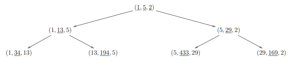

The correspondence between rationals and Markov numbers is determined by the values at and, following [8] (see Figures 2 and 3), these are by convention . Now, passing from these fractions to primitive lattice points we have the values of the norm at We can easily find the value at using Vieta flipping and we see that it is ie the same value as for . In fact one can go a step further and show that the three vectors correspond to the fundamental triple of Markov numbers . The unit ball of the associated stable norm looks just like the convex set depicted in Figure 1.
Now let be non negative real numbers as in the statement of Theorem 1.1. For any the point lies on the line . Since is a proper convex function this line meets the set
in exactly two points one of which is and the other has a negative coordinate. It follows that for the point is outside of the norm ball
and the first part of the theorem follows.
A similar argument using a vertical line instead of a horizontal one yields a proof of the second part of the Theorem 1.1.
Finally for the third part one must consider the line . It is easy to check that it meets in and and so for we have the required inequality.

References
- [1] M. Aigner, Markov’s theorem and 100 years of the uniqueness conjecture. A mathematical journey from irrational numbers to perfect matchings. Springer, Cham, 2013.
- [2] J. Berstel, A.Lauve, C. Reutenauer, F. Saliola. Combinatorics on Words: Christoffel Words and Repetitions in Words, CRM Monograph Series Volume: 27; 2008
- [3] Buser, Peter, and K -D. Semmler. The geometry and spectrum of the one holed torus. Commentarii Mathematici Helvetici 63.1 (1988): 259-274.
- [4] Harvey Cohn Approach to Markov’s Minimal Forms Through Modular Functions Annals of Mathematics Second Series, Vol. 61, No. 1 1955
- [5] William M Goldman The modular group action on real SL(2)–characters of a one-holed torus Geom. Topol. Volume 7, Number 1 (2003), 443-486.
- [6] Greg McShane, Hugo Parlier, Multiplicities of simple closed geodesics and hypersurfaces in Teichmüller space, Geom. Topol. Volume 12, Number 4 (2008), 1883-1919.
- [7] Greg McShane, Igor Rivin A norm on homology of surfaces and counting simple geodesics International Mathematics Research Notices, Volume 1995, Issue 2, 1995
- [8] M. Rabideaua, R. Schiffler, Continued fractions and orderings on the Markov numbers, Advances in Mathematics Vol 370, 2020.
- [9] C Lagisquet and E. Pelantová and S. Tavenas and L. Vuillon, On the Markov numbers: fixed numerator, denominator, and sum conjectures. https://arxiv.org/abs/2010.10335
- [10] Zagier, Don B. (1982). On the Number of Markov Numbers Below a Given Bound. Mathematics of Computation. 160 (160): 709–723